Single-photon scattering on a strongly dressed atom

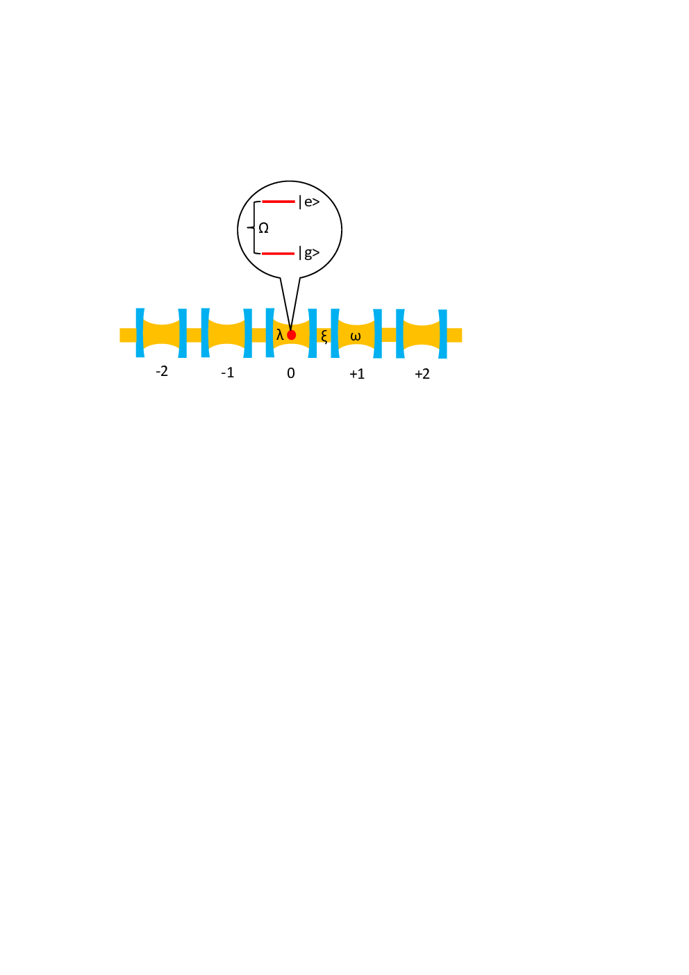
As shown in Fig. 1, we consider a $1$D array of infinite identical single-mode resonators with a TLS located inside a certain resonator, which is marked as the $0$-th resonator in the array. We further assume that the photons can hop between neighbor resonators. Then the total system is modeled by the Hamiltonian $H=H_{C}+H_{A}+H_{I}$, where the tight-binding Hamiltonian $H_{C}$ of the resonator array is

Here $\omega$ is the frequency of the photons in the resonators, $\xi$ is the hopping intensity or the inter-resonator coupling strength, $a_{j}$ and $a_{j}^{\dagger}$ are the annihilation and creation operators of the photons in the $j$-th resonator respectively.

In this paper we assume the weak-hopping condition

is satisfied. Therefore the term $a_{j}^{\dagger}a_{j+1}^{\dagger}+h.c.$ has been neglected in our consideration. This condition also provides us a small parameter $\xi/\omega$ which is very useful in the following calculation.

The Hamiltonian $H_{A}$ of the TLS and the interaction $H_{I}$ between the TLS and the photons in the $0$-th resonator are

and

respectively. Here $\Omega$ is the energy spacing between the ground state $|g\rangle$ and the excited state $|e\rangle$ of the TLS, $\lambda$ is the coupling intensity and the Pauli operators $\sigma_{z}$ and $\sigma_{x}$ are defined as $\sigma_{z}=\left|e\right\rangle\left\langle e\right|-\left|g\right\rangle\left\langle g\right|$ and $\sigma_{x}=\left|e\right\rangle\left\langle g\right|+\left|g\right\rangle\left\langle e\right|$.

In this and the next subsections, we develop the GRWA approach for the TLS-coupled 1D resonator array. To this end, in this section we first formally develop the adiabatic approximation for our system in the far-off resonance region with $\Omega<<\omega$. We will show that, due to the energy band structure of the photons, the adiabatic approximation cannot be used in our hybrid system, even in the far-off resonance case. However, as shown in the next subsection, we can also develop the GRWA approach as an improvement of this formal adiabatic approach, and the intrinsic problem of the adiabatic approximation in our system is naturally overcome by our GRWA approach. Finally, our approach is applicable in a broad parameter region, including the cases of $\Omega<<\omega$ and $\Omega\sim\omega$.

Under the far-off resonance condition $\Omega<<\omega$, the TLS is considered to be the slowly-varying part of the system, while the 1D resonator-array is the fast-varying one. Then we decompose the total Hamiltonian $H$ as $H=H_{1}+H_{2}$ where $H_{1}=H_{C}+H_{I}$ is the Hamiltonian of the fast-varying part together with the interaction and $H_{2}=H_{A}$ is the Hamiltonian of the slow-varying TLS.

The straightforward calculation shows that $H_{1}$ has the eigen-states

Here the TLS states $|\pm\rangle$ are the eigen-states of the operator $\sigma_{x}$ with eigen-values $\pm 1$, and $|0\rangle$ is the vacuum state of the resonator array. The photon momentum $k$ can take any value in the region $(-\pi,\pi],$ the creation operator $A(k)^{\dagger}$ for a photon with momentum $k$ is given by

and

is the set of all the numbers $n\left(k\right)$.

The operator $U$ in Eq. (5) is determined by

with $\mathcal{C}$ an unimportant c-number. This equation leads to the result

with

where

The results in Eqs.(10,11) are derived in appendix B. It is pointed out that the parameter $\alpha_{j}$ exponentially decays to zero in the limit $|j|\rightarrow\infty$.

Obviously, the eigen-energy of $H_{1}$ with respect to the eigen-state $|\pm,{\vec{n}}\rangle$ is

with

As shown in Fig. 2(a), in the weak-tunneling case with $\xi<<\omega$ the low-excited spectrum $E(\pm,{\vec{n}})$ of the eigen-energies of $H_{1}$ has a clear band structure. Each energy band includes all the energy levels with the same total photon number $N(\vec{n})$ and different photon-momentum distribution $\vec{n}$. The $N$-th energy band is centered at $N\omega$ with band width $4N\xi$. Therefore, in the low excitation cases the inter-band energy gap has the same order with $\omega$.

The spirit of the adiabatic approximation [63, 64, 65] is that, during the quantum evolution, the motion of the slowly-varying part of the system would follow the motion of the fast-varying one. Then the quantum state of the fast-varying 1D resonator array would be frozen in each adiabatic branch with fixed quantum number $\vec{n}$. Mathematically speaking, in the adiabatic approximation for our system, all the $H_{2}$-induced quantum transitions between the states $|\pm,\vec{n}\rangle$ and $|\pm,\vec{n^{\prime}}\rangle$ with $\vec{n}\neq\vec{n^{\prime}}$ are neglected. This treatment leads to the approximate eigen-states of the Hamiltonian $H$ as

Now we point out that, the adiabatic approximation is not a reasonable approximation for our present system, even in the case of $\Omega<<\omega$. That is because, the energy spectrum of $H_{1}$ has a band structure, each band includes all the states $|\pm,\vec{n}\rangle$ with the same total photon number $N(\vec{n})$. On the other hand, in the adiabatic approximation all the $H_{2}$-induced transitions between the eigen-states of $H_{1}$ with different quantum number ${\vec{n}}$ are neglected. It means that, all the inter-band transitions and the intra-band transitions between the states $|+,\vec{n}\rangle$ and $|-,\vec{n}^{\prime}\rangle$ with ${\vec{n}}\neq\vec{n}^{\prime}$ are omitted. In the case of $\Omega<<\omega$, the omission of inter-band transitions are reasonable because the energy gap between different bands is of the order of $\omega$, which is much larger than the intensity $\Omega$ of $H_{2}$. However, the neglecting of the intra-band transitions are unreasonable because the energy gaps between the levels in the same band can be arbitrary small.

As a comparison, we re-consider the simple system with a single-mode bosonic field interacting with a TLS. In Fig. 2(b), we plot the spectrum of the Hamiltonian

with $(a,a^{\dagger})$ the annihilation and creation operators of the bosonic field. It is apparent that in such a simple case the spectrum of $H_{\mathrm{Rabi1}}$ does not have any band structure (shown in appendix A). Therefore the adiabatic approximation [58] is applicable when $\Omega<<\omega$.

Although the adiabatic approximation cannot be used in our system, as shown in the next subsection, we can still develop the GRWA approach for our system with the help of the basis $\left\{|\Psi_{\pm,\vec{n}}\rangle\right\}$. Furthermore, in our GRWA approach the above intrinsic problem of the adiabatic approximation is naturally overcome.

Now we develop the GRWA approach for the system of the TLS-coupled 1D resonator array. Similar to the original GRWA for the single-mode bosonic field coupled to a TLS (appendix A), our general GRWA approach can also be considered as an improvement of the adiabatic approximation.

In our GRWA approach the total Hamiltonian $H$ is approximated as $H_{G}$ which is defined as

where the matrix elements $H_{{\vec{n}^{\prime}},\beta}^{{\vec{n}},\alpha}$ are defined as

while the symbol $\delta_{a,b}$ is defined as $\delta_{a,b}=1$ for $a=b$ and $\delta_{a,b}=0$ for $a\neq b$.

Apparently, in the approximate Hamiltonian $H_{G}$ we only take into account the quantum transitions between the states $|\Psi_{\alpha,{\vec{n}}}\rangle$ and $|\Psi_{\beta,{\vec{n}}^{\prime}}\rangle$ with

with $N_{\alpha}=1$ for $\alpha=+$ and $N_{\alpha}=0$ for $\alpha=-$. Obviously, this treatment is a direct generalization of the one in the development of the GRWA for the TLS-coupled single-mode bosonic field (shown in appendix A).

Furthermore, as proved in appendix C, we have

Then the intra-band transition only occurs between the states $|\Psi_{\alpha,{\vec{n}}}\rangle$ and $|\Psi_{\alpha,{\vec{n}}^{\prime}}\rangle$ with $N({\vec{n}})=N({\vec{n}^{\prime}})$. Therefore, all the intra-band transitions, which are unreasonably neglected in the adiabatic approximation, are included in our GRWA approach through the first term of the right hand side of Eq. (). Thus the intrinsic problem of the adiabatic approximation is overcome in our GRWAapproach. Therefore, our approach is applicable in the far-off resonance cases with $\Omega<<\omega$.

On the other hand, it is easy to prove that, under the near-resonance condition $\Omega\sim\omega$ and weak-coupling condition $|\lambda|<<\omega$, our GRWAapproach returns to the rotating-wave approximation. Therefore, as shown in Sec. III, our approach is applicable in a broad parameter region with $\Omega\lesssim\omega$.

Finally, we point out that, the approximate Hamiltonian $H_{G}$ in the GRWA approach in our case can also be re-expressed in a simple form

with $U$ given by Eq.(9) and $H_{R}^{\mathrm{RWA}}$ defined as

Here the operator $\hat{P}_{n}$ is defined as

where $|m_{l}\rangle_{l}$ is the Fock state of the $l$-th resonator with $m_{l}$ photons. It is apparent that $\hat{P}_{n}$ is the projection operator to the eigen-space of the total excitation operator

with respect to eigen-value $n$. In this sense, similarly to the GRWA for the TLS-coupled single-mode bosonic field discussed in appendix A, our GRWA approach can also be considered as “the rotating-wave approximation for the rotated Hamiltonian $U^{-1}HU$”.

The single-photon scattering amplitudes can be extracted from the asymptotic behavior of the eigen-state of the Hamiltonian $H$, which is approximated as $H_{G}$ in our GRWA approach. To this end, we need to solve the eigen-equation

with boundary conditions

in the limit of $j\rightarrow+\infty$. Here $|0\rangle_{-j}|0\rangle_{j}$ is the vacuum state of the resonator modes in the $j$-th and $-j$-th resonator, $|1\rangle_{-j}|0\rangle_{j}$ and $|0\rangle_{-j}|1\rangle_{j}$ are defined as $a_{-j}^{\dagger}|0\rangle_{-j}|0\rangle_{j}$ and $a_{j}^{\dagger}|0\rangle_{-j}|0\rangle_{j}$ respectively. $|\Phi(k)\rangle$ and $|\Phi^{\prime}(k)\rangle$ are the quantum states of the TLS and other resonators except the $\pm j$-th ones. $r_{k}$ and $t_{k}$ are the single-photon reflection and transmission amplitudes, or the single-photon scattering amplitudes.

The physical meaning of the boundary condition () can be understood as follows: For the scattering state with respect to a single photon input from the left of the $1$D resonator array, there are three possible relevant states for the $-j$-th and $j$-th resonators with large $|j|$, i.e., $|0\rangle_{-j}|0\rangle_{j}$, $|1\rangle_{-j}|0\rangle_{j}$ and $|0\rangle_{-j}|1\rangle_{j}$. Furthermore, the possibility amplitude with respect to $|1\rangle_{-j}|0\rangle_{j}$ is $\left(e^{ik\left(-j\right)}+r_{k}e^{-ik\left(-j\right)}\right)$, since the photon in the $-j$-th resonator can be either the input one or the reflected one. Similarly, the possibility amplitude with respect to $|0\rangle_{-j}|1\rangle_{j}$ is $t_{k}e^{ikj}$. It is easy to prove that the boundary condition used in the calculation of the single-photon scattering state with rotating-wave approximation (Eq. (5) of Ref. [2]) can be re-expressed as the one in Eq. ().

Usually the expression of $H_{G}$ in Eq. (20) is complicated and the eigen-equation (23) is difficult to be solved directly. However, due to Eq. (20), the Hamiltonian $H_{G}$ is related to $H_{R}^{\mathrm{RWA}}$ through a unitary transformation. Then the eigen-equation (23) of $H_{G}$ is equivalent to the one of $H_{R}^{\mathrm{RWA}}$:

and the eigen-state $|\Psi_{R}\left(k\right)\rangle$ of $H_{R}^{\mathrm{RWA}}$ is given by

More importantly, with the help of Eq.(9) and the fact that $\lim_{|j|\rightarrow\infty}\alpha_{j}=0$, the boundary condition (III.1) for $|\Psi\left(k\right)\rangle$ is transformed to the one of $|\Psi_{R}\left(k\right)\rangle$, i.e., in the limit of $j\rightarrow\infty$ we have

where $|\Phi_{R}\left(k\right)\rangle$ and $|\Phi_{R}^{\prime}\left(k\right)\rangle$ are defined as

and

respectively. Therefore, the scattering amplitudes $r_{k}$ and $t_{k}$ can be obtained from the solution of the eigen-equation (25) of $H_{R}^{\mathrm{RWA}}$ with boundary conditions (27).

In this subsection we solve the eigen-equation (25) of $H_{R}^{\mathrm{RWA}}$ and calculate the single-photon scattering amplitudes. To this end, we first use the explicit result about the unitary operator $U$ shown in appendix B to calculate the Hamiltonian $U^{-1}HU$. We have the results as:

with $\nu_{i}=-\alpha_{i}(a_{i}^{\dagger}-a_{i})$. In principle, we can derive the explicit expression of $H_{R}^{\mathrm{RWA}}$ with Eqs. (21) and (). Here, for simplicity, we expand $H_{R}^{\mathrm{RWA}}$ as a power series of the parameter $\xi/\omega$ and only keep the low-order terms under the weak-hopping condition $\xi<<\omega$. Then we can analytically solve Eq. (25) with the approximated $H_{R}^{\mathrm{RWA}}$ and derive the single-photon scattering amplitudes.

Now we calculate the single-photon scattering amplitudes with first-order approximation where only the $0$-th order and $1$-st order terms of $\xi/\omega$ are kept in $H_{R}^{\mathrm{RWA}}$. As shown in the following, in most of the cases, this approximation is enough to give accurate results for the scattering amplitudes. The straightforward calculation shows that, up to the first order of $\xi/\omega$, $H_{R}^{\mathrm{RWA}}$ is approximated as

with the parameters

The physical meaning of Eq.(31) is very clear. In the $0$-th order terms of $\xi/\omega$, or the terms proportional to $\omega_{0g}^{\left(0\right)}$, $\omega_{0e}^{\left(0\right)}$, $\omega_{1g}^{\left(0\right)}$ and $J^{\left(0\right)}$, the effective couplings occur between the TLS and the photon in the $0$-th resonator in which the TLS is located. Nevertheless, in the $1$-st order terms proportional to $J^{\left(1\right)}$, effective couplings appear between the TLS and the modes in the $\pm 1$-st resonators. These terms imply that the non-rotating-wave effects from the coupling between the TLS and the $0$-th resonator can indirectly influence the behavior of the modes in the $\pm 1$-st resonators. Furthermore, the hopping intensities between the $0$-th and $\pm 1$-st resonators are also tuned by the terms with $\omega_{1g}^{\left(1\right)}$.

As shown above, the single-photon scattering amplitudes are approximately derived from the eigen-equation

of $H_{R}^{\mathrm{RWA}\left(1\right)}$ with boundary condition (27). It is apparent that the solution $|\Psi_{R}\left(k\right)\rangle$ of Eq.(33) takes the form

with the coefficients $u_{k}^{\left(1\right)}(j)$ given by

Substituting Eqs.(34,35) into Eq.(33), we obtain the linear equations for the reflection amplitude $r_{k}^{\left(1\right)}$ and transmission amplitude $t_{k}^{\left(1\right)}$. These equations can be solved analytically. Then we obtain the scattering amplitudes $r_{k}^{\left(1\right)}$ and $t_{k}^{\left(1\right)}$ given by the first-order approximation of $H_{R}^{\mathrm{RWA}}$:

The above procedure can be straightforwardly generalized to the cases with high-order approximations of $H_{R}^{\mathrm{RWA}}$. For instance, in the second-order approximation, $H_{R}^{\mathrm{RWA}}$ is approximated as $H_{R}^{\mathrm{RWA}\left(2\right)}$ which includes the $0$-th order, $1$-st order and $2$-nd order terms of $\xi/\omega$. It can be found that in $H_{R}^{\mathrm{RWA}\left(2\right)}$ the TLS is effectively coupled to the $0$-th, $\pm 1$-st and $\pm 2$-nd resonators. We can also solve the eigen-equation of $H_{R}^{\mathrm{RWA}\left(2\right)}$, and obtain the analytical expressions of the relevant scattering amplitudes $r_{k}^{\left(2\right)}$ and $t_{k}^{\left(2\right)}$. In general, for any integer $n$, the scattering amplitudes $r_{k}^{\left(n\right)}$ and $t_{k}^{\left(n\right)}$ from the $n$-th order approximation of $H_{R}^{\mathrm{RWA}}$ can be obtained with the similar approach. In the limit of $n\rightarrow\infty,$ the results $r_{k}^{\left(n\right)}$ and $t_{k}^{\left(n\right)}$ would converge to fixed values $r_{k}$ and $t_{k}$ or the precise values of the single-photon scattering amplitudes.

In Figs. 3 and 4, we illustrate the single-photon scattering amplitude $r_{k}$ given by our GRWA approach with the first and second order approximations, i.e., $r_{k}^{(1)}$ and $r_{k}^{(2)}$, the one given by the rotating-wave approximation and the result from the numerical diagonalization of the rotated Hamiltonian $U^{-1}HU$. In our numerical calculations the total excitation defined in (22) is cut off at a given number $C_{p}$ for the Hamiltonian $U^{-1}HU$, and the results with $C_{p}=2,\ 3$ are shown in our figures.

In Fig. 3 we calculate the reflection rate $|r_{k}|^{2}$. It is clearly shown that the results $|r_{k}^{(1)}|^{2}$ and $|r_{k}^{(2)}|^{2}$ from the first and second order approximation for $(\xi/\omega)$ consist very well with each other. Therefore, in most of the cases with $|\xi|<<\omega,$ the first order approximation is good enough for our GRWA approach.

Furthermore, it is shown that in the case of Fig. 3(a) where the weak-coupling and near-resonance conditions are satisfied, both the results from the rotating-wave approximation and our GRWA approach fit well with the numerical calculations. Nevertheless, in the cases of Figs. 3(b)-3(d) where the rotating-wave approximation is not applicable, the results from our GRWA approach also consist significantly well with the numerical calculations. This observation is further confirmed by Fig. 4 where the real and imaginary parts of $r_{k}$ given by different approaches are illustrated.

In Figs. 3(b) and 3(d) with $\Omega=0.4\omega$, we also compare our results with the ones given by the adiabatic approximation. It is shown that as we argued in Sec. II, the adiabatic approximation may be not applicable even when $\Omega<<\omega$, while our GRWA approach can still provide reasonable results.

Therefore, the results in Figs. 3 and 4 show that, our GRWA approach with the first-order approximation for $(\xi/\omega)$, or our results $r_{k}^{(1)}$ and $t_{k}^{(1)}$ in Eqs. (III.2, 42) can be used as a good analytical approximation for the single-photon scattering amplitudes in the parameter region with $|\xi|<<\omega$ and $\Omega\lesssim\omega$.

References

- [1] J. T. Shen and S. Fan, Phys. Rev. A 76, 062709 (2007).
- [2] L. Zhou, Z. R. Gong, Y. X. Liu, C. P. Sun, and F. Nori, Phys. Rev. Lett. 101, 100501 (2008).
- [3] D. Z. Xu, H. Ian, T. Shi, H. Dong, and C. P. Sun, Science China Physics Mechanics and Astronomy 53, 1234 (2010).
- [4] X. F. Zang and C. Jiang, J. Phys. B, 43, 215501 (2010).
- [5] J. Lu, L. Zhou, H. C. Fu, and L. M. Kuang, Phys. Rev. A 81, 062111 (2010).
- [6] M. T. Cheng, Y. Y. Song, Y. Q. Luo, and G. X. Zhao, Comm. Theor. Phys. 55, 501 (2011).
- [7] Y. F. Xiao, J. Gao, X. B. Zou, J. F. McMillan, X. Yang, Y. L. Chen, Z. F. Han, G. C. Guo and C. W. Wong, New. J. Phys., 10, 123013 (2008).
- [8] L. Zhou, H. Dong, Y. X. Liu, C. P. Sun, and F. Nori, Phys. Rev. A 78, 063827 (2008).
- [9] Y. Chang, Z. R. Gong, and C. P. Sun, Phys. Rev. A 83, 013825 (2011).
- [10] F. M. Hu, L. Zhou, T. Shi, and C. P. Sun, Phys. Rev. A 76, 013819 (2007).
- [11] P. B. Li, Y. Gu, Q. H. Gong, and G. C. Guo, Phys. Rev. A 79, 042339 (2009).
- [12] L. Zhou, Y. B. Gao, Z. Song, and C. P. Sun, Phys. Rev. A 77, 013831 (2008).
- [13] J. Q. Liao, J. F. Huang, Y. X. Liu, L. M. Kuang, and C. P. Sun, Phys. Rev. A 80, 014301 (2009).
- [14] J. Q. Liao, Z. R. Gong, L. Zhou, Y. X. Liu, C. P. Sun, and F. Nori, Phys. Rev. A 81, 042304 (2010).
- [15] Z. R. Gong, H. Ian, L. Zhou, and C. P. Sun, Phys. Rev. A 78, 053806 (2008).
- [16] M. X. Huo, Y. Li, Z. Song, and C. P. Sun, Phys. Rev. A 77, 022103 (2008).
- [17] M. Patterson, S. Hughes, S. Combri, N. V. Q. Tran, A. D. Rossi, R. Gabet, and Y. Jaoun, Phys. Rev. Lett. 102, 253903 (2009).
- [18] P. Longo, P. Schmitteckert, and K. Busch, J. Opt. A 11, 114009 (2009).
- [19] M. Alexanian, Phys. Rev. A 81, 015805 (2010).
- [20] J. Q. Quach, C. H. Su, A. M. Martin, A. D. Greentree, and L. C. L. Hollenberg, Optics Express 19, 11018 (2011).
- [21] T. Shi and C. P. Sun, arXiv: 0907.2776.
- [22] P. Longo, P. Schmitteckert, and K. Busch, Phys. Rev. Lett. 104, 023602 (2010).
- [23] P. Longo, P. Schmitteckert, and K. Busch, Phys. Rev. A 83, 063828 (2011).
- [24] D. Roy, Phys. Rev. A 83, 043823 (2011).
- [25] L. Zhou, S. Yang, Y. X. Liu, C. P. Sun, and F. Nori, Phys. Rev. A 80, 062109 (2009).
- [26] Z. Ji and S. Gao, arXiv:1107.1934.
- [27] D. Roy, Phys. Rev. Lett. 106, 053601 (2011).
- [28] H. Dong, Z. R. Gong, H. Ian, L. Zhou, and C. P. Sun, Phys. Rev. A 79, 063847 (2009).
- [29] J. T. Shen and S. Fan, Phys. Rev. Lett. 95, 213001 (2005).
- [30] J. T. Shen and S. Fan, Phys. Rev. A 79, 023838 (2009).
- [31] X. F. Zang, and C. Jiang, J. Phys. B, 43, 065505 (2010).
- [32] E. Rephaeli, J. T. Shen, and S. Fan, Phys. Rev. A 82, 033804 (2010).
- [33] J. T. Shen and S. Fan, Phys. Rev. A 79, 023837 (2009).
- [34] Y. L. Chen, Y. F. Xiao, X. Zhou, X. B. Zou, Z. W. Zhou and G. C. Guo, J. Phys. B: At. Mol. Opt. Phys. 41, 175503 (2008).
- [35] G. Romero, J. J. García-Ripoll, and E. Solano, Physica Scripta t137, 014004 (2009).
- [36] G. Romero, J. J. García-Ripoll, and E. Solano, Phys. Rev. Lett. 102, 173602 (2009).
- [37] E. Rephaeli, S. E. Kocabas, and S. Fan, arXiv:1112.1428.
- [38] J. Lu, H. Dong, and L. M. Kuang, Comm. Theor. Phys. 52, 500 (2009).
- [39] J. T. Shen and S. Fan, Phys. Rev. Lett. 98, 153003 (2007).
- [40] J. T. Shen and S. Fan, Opt. Lett. 30, 2001 (2005).
- [41] T. S. Tsoi and C. K. Law, Phys. Rev. A 80, 033823 (2009).
- [42] T. Shi and C. P. Sun, Phys. Rev. B 79, 205111 (2009).
- [43] T. Shi, S. Fan, and C. P. Sun, Phys. Rev. A 84, 063803 (2011).
- [44] H. X. Zheng, D. J. Gauthier, and H. U. Baranger, Phys. Rev. A 82, 063816 (2010).
- [45] D. Roy, Phys. Rev. B 81, 155117 (2010).
- [46] S. Fan, S. E. Kocabas, and J. T. Shen, Phys. Rev. A 82, 063821 (2010).
- [47] I. C. Hoi, C. M. Wilson, G. Johansson, T. Palomaki, B. Peropadre, and P. Delsing, Phys. Rev. Lett. 107, 073601 (2011).
- [48] D. Witthaut and A. S. Srensen, New J. Phys. 12, 043052 (2010).
- [49] J. Q. Liao and C. K. Law, Phys. Rev. A 82, 053836 (2010).
- [50] A. Faraon, E. Waks, D. Englund, I. Fushman, and J. Vukovi, App. Phys. Lett. 90, 073102 (2007).
- [51] Y. Akahane, T. Asano, B. S. Song, and S. Noda, Nature 425, 944 (2003).
- [52] A. Wallraff, D. I. Schuster, A. Blais, L. Frunzio, R.-S. Huang, J. Majer, S. Kumar, S. M. Girvin, and R. J. Schoelkopf, Nature (London) 431, 162 (2004).
- [53] M. Devoret, S. M. Girvin, and R. Schoelkopf, Ann. Phys. (Leipzig) 16, 767 (2007).
- [54] R. J. Schoelkopf and S. M. Girvin, Nature (London) 451, 664 (2008).
- [55] J. Bourassa, J. M. Gambetta, A. A. Abdumalikov, O. Astafiev, Y. Nakamura, and A. Blais, Phys. Rev. A 80, 032109 (2009).
- [56] C. Ciuti, G. Bastard, and I. Carusotto, Phys. Rev. B 72, 115303 (2005).
- [57] E. K. Irish, Phys. Rev. Lett. 99, 173601 (2007).
- [58] E. K. Irish, J. G. Banacloche, I. Martin, and K. C. Schwab, Phys. Rev. B 72, 195410 (2005).
- [59] C. P. Sun, Science in China (Series A) 38, 2 (1995).
- [60] J. Hausinger and M. Grifoni, Phys. Rev. A 82, 062320 (2010).
- [61] D. Braak, Phys. Rev. Lett. 107, 100401 (2011).
- [62] E. T. Jaynes and F. W. Cummings, Proc. IEEE 51 (1): 89 (1963).
- [63] M. Born and R. Oppenheimer, Ann. Phy. 84, 457 (1930).
- [64] C. P. Sun and M. L. Ge, Phys. Rev. D 41, 1349, (1990).
- [65] P. Zhang, Y. D. Wang, and C. P. Sun, arXiv: quant-ph/0401058.