Optimal Server Assignment in Multi-Server Queueing Systems with Random Connectivities

The problem of throughput-optimal server allocation in multi-queue, single-server systems with random connectivities was addressed in [2, 20, 10, 21]. In [2], the authors considered a time-slotted, multi-queue single-server system with Bernoulli packet arrivals and connectivities from each of the queues to a single server. They introduced LCQ (Longest Connected Queue) policy as a throughput-optimal policy and also characterized the stability region by a set of linear inequalities. The authors in [20] considered a continuous-time version of the model studied in [2] with finite buffer space and showed that under stationary ergodic input job flow and modulation processes, LCQ policy maximizes the stable throughput region of this system. In [10], C-FES (Connected queue with the Fewest Empty Spaces) policy, a policy that allocates the server to the connected queue with the fewest empty spaces, was introduced for this system. It was shown that C-FES stochastically minimizes the loss flow and maximizes the throughput of the system. In [21], a model similar to the model of [10, 2] was studied and it was shown that the Best User (BU) policy maximizes the expected discounted number of successful transmissions.

While in throughput-optimal server allocation the objective is to find a policy that maximizes the throughput region of the system and keeps the queues stable [1, 4], in delay-optimal server allocation the goal is to determine a policy that minimizes the average queueing delay. Thus, the objective in delay optimality is more stringent than the objective in throughput optimality. A server allocation policy may be throughput-optimal but not delay-optimal; however, a delay-optimal policy (for all the arrival rates) is always throughput-optimal. In [2], the authors (other than proving the throughput optimality of LCQ as mentioned earlier) proved that for a multi-queue, single-server system with i.i.d. Bernoulli arrival and connectivity processes, the LCQ policy is also delay-optimal. The extension of this result for non-i.i.d. case is still an open problem.

In generalizing the results to multi-queue, multi-server (MQMS) systems, various multi-server systems have been studied [22, 15, 16, 3, 23, 24, 25]. In [22], Maximum Weight (MW) policy was proposed as a throughput-optimal server allocation policy for an MQMS queueing system with general, stationary channel processes. MW policy can be considered as a special case of back-pressure algorithm which was proven in [1, 4] to be a throughput-optimal resource allocation algorithm in a general queueing system. In [15], the authors characterized the network stability region of multi-queue, multi-server systems with time-varying, independent connectivities. The results were further extended in [16] for more general, stationary channel distributions (and not just independent Bernoulli channels). In all the models studied in [22, 15, 16], there is no restriction on the number of servers that can be allocated to a queue. For ease of reference, we will call such an MQMS system as MQMS-Type1. In [3], it was shown that for an MQMS system in which the queues are restricted to get service from at most one server during each time slot, Maximum Weighted Matching (MWM) policy is throughput-optimal. For ease of reference, we will call such an MQMS system with this extra assumption as MQMS-type2. The authors also considered the effect of infrequent channel state measurements on the network stability region of MQMS systems. Similar to MQMS-Type1, for MQMS-Type2 the throughput-optimal policy (MWM) can be considered as a special case of the back-pressure algorithm.

In contrast to the single-server system (where LCQ was both throughput-optimal and delay-optimal), in MQMS-Type1 system the MW policy is not necessarily delay-optimal. More specifically, in [15] it was also shown that although MW policy is throughput-optimal, even for a system with i.i.d. Bernoulli arrivals and connectivity processes, MW policy in its general form, is not delay-optimal.

The delay-optimal server allocation problem in multi-server systems was addressed in [23, 24, 25]. The authors in [23] considered a queueing model with a set of parallel queues and i.i.d. Bernoulli packet arrivals that are competing to attract service from $K$ identical servers forming a server-bank. The connectivities of the queues to the entire server-bank are assumed to be i.i.d. Bernoulli processes. Each queue is restricted to receive service from at most one server during each time slot. The authors proposed LCQ policy in which the servers of the server-bank are allocated to the $K$ longest connected queues at each time slot. Using dynamic coupling and stochastic ordering, they proved the delay optimality of LCQ policy for such a system. In our work, the focus would be on delay optimality of MWM policy in MQMS-Type2 system in which the servers are not restricted to form a server-bank. Instead, we assume that each queue has an independent connectivity to each individual server (as seen in Figure 1). The work in [24, 25] focuses on delay optimal server allocation problem in the MQMS-Type1 system. In [24], the authors introduced MTLB (Maximum-Throughput Load-Balancing) policy and using dynamic programming showed that this policy minimizes a class of cost functions including total average delay for the case of two queues with i.i.d., Bernoulli-distributed arrivals and connectivities. In [24], no general argument was provided for the optimality of MTLB for more than two queues. The work in [25] considers this problem for a general number of queues and servers. In [25], a class of Most Balancing (MB) policies was characterized among all work-conserving policies which minimize, in stochastic ordering sense, a class of cost functions including total queue occupancy (and thus are delay-optimal). However, this class of proposed MB policies is just characterized by a property of this class; the authors did not introduce an explicit implementation for the optimal policy. In this paper, we focus on MWM policy and prove that this throughput-optimal policy is also delay-optimal for an MQMS-Type2 system with i.i.d. arrival and connectivity processes. Our work extends the results derived in [2, 23]. In particular, the researchers in [2, 23] have considered queueing models where a single server or a server-bank is randomly connected to a set of parallel queues. In this paper, we consider a more general model where each individual server is randomly connected to the queues (as seen in Figure 1). Although the two models bear certain similarities, extending the results from single-server (server-bank) system to multi-server system is not a straightforward procedure. Our work is different from the work in [2, 23] from both the modeling power and the difficulty in proof points of view.

For more information on optimal scheduling and resource allocation problems in wireless networks the reader is encouraged to also consult with [4, 26, 27, 28, 29, 30].

Our contributions in this paper are summarized as follows: First, for an MQMS-Type2 system we prove that during each time slot, Maximum Weighted Matching (MWM) policy will result in the most balanced queue vector in the system, i.e., maximization of the matching weight and balancing of the queues are equivalent. Graph theoretic arguments were applied to prove this result that is formally introduced in Lemma 1 and Lemma 2 later in the paper. Note that our approach to prove this result is only applicable to the MQMS-Type2 model (due to the structure of the model and the MWM policy) and cannot be easily extended to MQMS-Type1 system. Second, using this result in conjunction with the notions of stochastic ordering and dynamic coupling, we prove the delay optimality of MWM policy for an MQMS-Type2 system with i.i.d. Bernoulli arrivals and connectivities. More specifically, we prove that MWM minimizes, in stochastic ordering sense, a range of cost functions of queue lengths including total queue occupancy¹¹ 1 The optimality of MWM is proven among all causal server assignment policies.. Third, we then extend our model by considering imperfect services where it is assumed that the service of a scheduled packet fails randomly with a certain probability. We prove that MWM is still optimal for the extended model. We finally show that the results are still valid for some more general connectivity and arrival processes which follow conditional permutation invariant distributions.

The rest of this paper is organized as follows. In Section II, we introduce the queueing model and the required notation. In Section III, we describe the Maximum Weighted Matching (MWM) server assignment policy. In Section IV, we prove the delay optimality of MWM server assignment policy. In Section V, we present simulation results where we compare the performance of MWM policy with the performance of two other server assignment policies in terms of average total queue occupancy (or equivalently average queueing delay). Finally, we summarize our conclusions in Section VI.

At each time slot $t$ the server assignment policy has to decide about a bipartite (graph) matching⁴⁴ 4 A matching in a bipartite graph is a sub-graph of the original graph in which no two edges share a common vertex. between sets $\cal N$ and $\cal K$. We assume that this decision is made in a causal fashion, i.e., based on the available history of arrival processes, service processes, queue states and the connectivity states until time $t$.

A policy $\pi$ is fully determined by its indicator variables $M^{(\pi)}_{n,k}(t)~\forall n\in\mathcal{N},\forall k\in\mathcal{K},t=1,2,\dots$ which are defined as

We define the $N\times K$ matrix $\boldsymbol{M}^{(\pi)}(t)=(M^{(\pi)}_{n,k}(t)),\forall n\in\mathcal{N},\forall k\in\mathcal{K}$ as the employed matching by policy $\pi$ at time slot $t$. Hence, a server assignment policy $\pi$ can be defined as the set of all the employed matchings by policy $\pi$ at time slots $t=1,2,\dots$, i.e., $\pi=\{\boldsymbol{M}^{(\pi)}(t)\}_{t=1}^{\infty}$. We denote the matching space containing all the possible assignments of the servers to the queues by $\cal M$. The set $\mathcal{M}$ is equivalent to the set of all the possible matchings in an $N\times K$ complete bipartite graph⁵⁵ 5 A complete bipartite graph is a bipartite graph in which each vertex in each part is connected to all the vertices in the other part. An $N\times K$ bipartite graph has $NK$ edges..

We can observe that $X_{n}(t)$, the queue length random variable, evolves in time as follows:

The operator $(\cdot)^{+}$ returns the term inside the parentheses if it is non-negative and zero otherwise.

The queueing model introduced in this section is useful in providing intuition for modeling resource assignment problems in various systems with shared resources [17, 3]. In wireless communication systems, resources such as communication sub-channels, relay stations, etc. are shared among users. As an example, we can consider a relaying access network with $N$ users and $K$ shared relays. By modeling the cooperative wireless channel between each user, each relay and the base station as an erasure channel, the performance of such a system can be studied following our model in Figure 2.

In [1, 4], it was shown that back-pressure algorithm maximizes the stable throughput region of a general data network, i.e., it is throughput-optimal. The reader may refer to [1, 4] for more information about back-pressure algorithm. For the model introduced in Section II, the back-pressure algorithm reduces to the following optimization problem at each time slot $t$ [3]. In this integer programming problem, $M_{n,k}(t)$ variables are the optimization variables and $X_{n}(t-1)$ and $C_{n,k}(t)$ are known parameters.

Finding the solution of problem (3) is equivalent to finding a maximum weighted matching in the $N\times K$ bipartite graph $G_{t}=(\mathcal{N},\mathcal{K},\mathcal{E})$ shown in Figure 3. Hence, the back-pressure algorithm for the queueing model of Figure 2 is also known as Maximum Weighted Matching (MWM) algorithm. In $G_{t}$, $\mathcal{N}$ and $\mathcal{K}$ are the two sets of vertices in each part of the graph and $\mathcal{E}=\{e_{n,k},\forall n\in\mathcal{N},\forall k\in\mathcal{K}\}$ is the set of edges between these two parts. In $G_{t}$, the associated weight to each edge $e_{n,k}$ is $X_{n}(t-1)C_{n,k}(t)$. A matching in graph $G_{t}$ is a sub-graph of $G_{t}$ in which no two edges share a common vertex. Any matching $\boldsymbol{M}^{(\pi)}(t)$ at any time slot $t$ is corresponding to a sub-graph of $G_{t}$ namely $G_{t}^{(\pi)}=(\mathcal{N},\mathcal{K},\mathcal{E}^{(\pi)})$ in which $e_{n,k}\in\mathcal{E}^{(\pi)}$ if and only if $M^{(\pi)}_{n,k}(t)=1$. There are several algorithms to find the maximum weighted matching in bipartite graphs. The most well-known one is the Hungarian algorithm with $O((\min\{N,K\})(\max\{N,K\})^{2})$ complexity [31].

Assume that $\boldsymbol{M}^{(\text{MWM})}(t)=(M^{(\text{MWM})}_{n,k}(t))~\forall n\in\mathcal{N},\forall k\in\mathcal{K}$ is the matching whose indicator variables are the solution of the optimization problem (3). $\boldsymbol{M}^{(\text{MWM})}(t)$ has the following properties:

• (a)

  $\boldsymbol{M}^{(\text{MWM})}(t)$ always exists at all time slots.

• (b)

  The maximum weighted matching in a bipartite graph may not be unique, i.e., there may be more than one matching $\boldsymbol{M}^{(\text{MWM})}(t)$ for the graph of Figure 3 at each time slot.

An MWM policy at each time slot observes the queue lengths $X_{n}(t-1)$ and the connectivity variables $C_{n,k}(t)$ and determines a maximum weighted matching (the matching indicator variables) in the bipartite graph of Figure 3. Note that, by construction, the MWM policy is causal.

According to property (a) above, the set $\Pi^{\text{MWM}}$ is not empty. Moreover, according to property (b), we conclude that $\Pi^{\text{MWM}}$ may contain an infinite number of policies.

First, We will introduce the notion of balanced queue vectors and the corresponding balancing server reallocation at time slot $t$ in Definition 4. For any given policy $\pi$ and a fixed time slot $t$, we will also define the Matching Weight index $\mathsf{MW}_{\pi}(t)$ in Definition 5. Note that this index is not directly related to (average) delay; it is, however, a crucial link in comparing arbitrary policies to the MWM ones in the set $\Pi^{\text{MWM}}$ defined in the previous section. We show then in Lemmas 1 and 2 that the notions of “maximizing the Matching Weight index” and “producing balanced queue vectors” via balancing server reallocations are equivalent. This property allows us to characterize MWM policies as ones that produce the most balanced queue size vectors possible.

Second, we use the balanced queue size property to show in Lemma 3 that for any arbitrary policy $\pi$ outside the set $\Pi^{\text{MWM}}$, we may construct a policy in the set $\Pi^{\text{MWM}}$ that improves $\pi$ in terms of delay. In the words of Theorem 1, we prove that the delay-optimal policy belongs to the set of MWM policies $\Pi^{\text{MWM}}$.

Third, in Lemmas 4 and 5 we will show that all policies in the set $\Pi^{\text{MWM}}$ result in the same cost (and hence average delay). Finally, by using Theorem 1 and Lemma 4 we conclude Theorem 2 where we show that the policies in the set $\Pi^{\text{MWM}}$ are all delay-optimal. Graph theoretic analysis is applied in the proof of Lemmas 2 and 5 and stochastic ordering and dynamic coupling arguments are used to prove Lemmas 3 and 4.

We start this section by introducing the intermediate queue state in the following definition.

Given $\boldsymbol{x}^{\prime}(t)$ as a sample value of random vector $\boldsymbol{X}^{\prime}(t)$, we define a balancing server reallocation at time slot $t$ as follows.

A balancing server reallocation is a crucial tool in defining new policies that improve the delay performance of an arbitrary policy as we will see in the proof later.

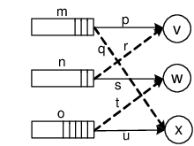
Example: Consider a system with three queues and three servers. Assume that $\boldsymbol{x}(t-1)=(3,2,5)$ is the queue length vector right at the end of time slot $t-1$ (or at the beginning of time slot $t$). We consider two distinct examples to show the definition of balancing server reallocations corresponding to each of the cases C1 and C2 in Definition 4. Figures 5a and 5b show these examples of balancing server reallocations. In each case, we also show the weight of each edge $(n,k)$ which is equal to $c_{n,k}(t)x_{n}(t-1)$. In these figures, since none of the queues is empty, the edges with weight $0$ are the ones which are disconnected. We have specified the original allocations by solid lines and the balancing ones by dashed lines. For the system in Figure 5a, the original allocation will result in the intermediate vector $\boldsymbol{x}^{\prime}(t)=(3,1,4)$ while the balancing server reallocation will result in the intermediate vector $\tilde{\boldsymbol{x}}^{\prime}(t)=(2,1,4)$. The vectors $\boldsymbol{x}^{\prime}(t)$ and $\tilde{\boldsymbol{x}}^{\prime}(t)$ satisfy Condition C1. For the system in Figure 5b, the original allocation will result in the intermediate vector $\boldsymbol{x}^{\prime}(t)=(2,1,5)$ while the balancing server reallocation will result in $\tilde{\boldsymbol{x}}^{\prime}(t)=(3,1,4)$. The vectors $\boldsymbol{x}^{\prime}(t)$ and $\tilde{\boldsymbol{x}}^{\prime}(t)$ satisfy Condition C2.

$\mathsf{MW}$ index is exactly the objective of the optimization problem (3). $\mathsf{MW}_{\pi}(t)$ is an index associated with policy $\pi$ at time slot $t$ whose value is dependent on the state of the system (queue lengths and connectivities) as well as the matching employed by policy $\pi$ at time slot $t$. In the following lemmas (Lemmas 1 and 2), we relate the notions of balancing server reallocation and Matching Weight index and we prove that maximization of $\mathsf{MW}_{\pi}(t)$ index and balancing of the queues are equivalent. More specifically, we show that if the $\mathsf{MW}_{\pi}(t)$ index for policy $\pi$ is not maximized at time slot $t$ ($\pi$ is not using a maximum weighted matching), then there exists a balancing server reallocation (i.e., a new matching that satisfies either C1 or C2) that results in a larger $\mathsf{MW}$ index. Furthermore, if $\pi$ is using a maximum weighted matching, then there exists no balancing server reallocation at that time slot, i.e., no matching can be found that satisfies either C1 or C2. These facts are formally stated in the following two lemmas.

The detailed proof of the lemma is given in Appendix A-A. Based on Lemma 1, we can state the following corollary.

In this section, we briefly review the concepts of stochastic ordering (stochastic dominance) and dynamic coupling techniques. These concepts are needed in the proof of delay optimality of MWM policy in the rest of our discussion. The reader is encouraged to consult [32, 33, 34] for more details about stochastic ordering and dynamic coupling.

The following two properties of stochastic ordering are useful: if $A\leq_{st}B$, then

• (a)

  $E[A(t)]\leq E[B(t)]$

• (b)

  $f(A)\leq_{st}f(B)$ for all non-decreasing functions $f$.

Process $A$ is stochastically smaller than $B$, if there exists a process $\tilde{A}=\{\tilde{A}(t)\}_{t=1}^{\infty}$ defined on the same probability space as $B$, has the same probability distribution as $A$ and satisfies $\tilde{A}(t)\leq B(t)$ almost surely (a.s.) for every $t=1,2,\dots$ [23]. The last statement is known as coupling of $A$ and $\tilde{A}$. When applying coupling technique, given the process $A$, we construct a coupled process $\tilde{A}$ with the same distribution as $A$ and $\tilde{A}(t)\leq B(t)$ a.s. for all $t$. This gives us a tool for comparing the processes $A$ and $B$ stochastically when it is infeasible to derive the distributions of $A$ and $B$ (e.g., in our queueing model when comparing the total occupancy process for different server assignment policies).

In this subsection, we will elaborate on proving the delay optimality of any MWM policy. We first introduce some definitions. We denote by $\mathbb{Z}_{+}$ the set of non-negative integers and by $\mathbb{Z}_{+}^{N}$ the $N$ dimensional Cartesian space of non-negative integers. We define the relation “$\preceq$” on $\mathbb{Z}_{+}^{N}$ as follows.

The three relations D1, D2 and D3 are mutually exclusive. In D3, we say that $\tilde{\boldsymbol{x}}$ is more balanced than $\boldsymbol{x}$ and can be obtained by decreasing a larger element of $\boldsymbol{x}$ (i.e., $m$) by one and increasing a smaller element (i.e., $n$) by one. We call such an interchange as a balancing interchange on vector $\boldsymbol{x}$. Thus, the result of a balancing interchange on a vector $\boldsymbol{x}$ would be a vector $\tilde{\boldsymbol{x}}$ such that $\tilde{\boldsymbol{x}}\preceq\boldsymbol{x}$. According to Definition 4, a balancing server reallocation satisfying Condition C2, will result in a balancing interchange between $\boldsymbol{x}^{\prime}(t)$ and $\tilde{\boldsymbol{x}}^{\prime}(t)$.

We define the partial order “$\preceq_{p}$” on $\mathbb{Z}_{+}^{N}$ as the transitive closure of relation“ $\preceq$” [35]. In other words, $\tilde{\boldsymbol{x}}\preceq_{p}\boldsymbol{x}$ if and only if $\tilde{\boldsymbol{x}}$ is obtained from $\boldsymbol{x}$ by performing a sequence of reductions (i.e., reducing an element of the vector $\boldsymbol{x}$ such that $\boldsymbol{x}$ and $\tilde{\boldsymbol{x}}$ satisfy D1), permutations of two elements (permutation of two elements of the vector $\boldsymbol{x}$ such that $\boldsymbol{x}$ and $\tilde{\boldsymbol{x}}$ satisfy D2) and/or balancing interchanges (such that $\boldsymbol{x}$ and $\tilde{\boldsymbol{x}}$ satisfy D3). When $\boldsymbol{x}$ and $\tilde{\boldsymbol{x}}$ are two queue length vectors, we write $\tilde{\boldsymbol{x}}\preceq_{p}\boldsymbol{x}$ if and only if queue length vector $\tilde{\boldsymbol{x}}$ is obtained from $\boldsymbol{x}$ by applying a sequence of packet removals, two-queue permutations and balancing interchanges.

We can easily check that function $f(\boldsymbol{x})=\sum_{n=1}^{N}x_{n}$ belongs to $\cal F$. This function represents the total queue occupancy of the system.

We observe that $\Pi_{t-1}\supseteq\Pi_{t}$ and $\Pi^{\text{MWM}}=\bigcap_{t=1}^{\infty}\Pi_{t}$.

Consider a policy $\pi\in\Pi_{t-1}$ which is using an arbitrary matching $\boldsymbol{M}^{(\pi)}(t)$ at time slot $t$. If $\boldsymbol{M}^{(\pi)}(t)$ is not a maximum weighted matching, then from Lemmas 1 and 2 we conclude that by applying a sequence of balancing server reallocations⁶⁶ 6 According to Lemma 1, each balancing server reallocation strictly increases the matching weight index. we can create a policy $\pi^{\star}\in\Pi_{t}$. Let $h_{t}^{\pi}$ denote the number of balancing server reallocations required to convert the employed matching in policy $\pi$ at time slot $t$ to a maximum weighted matching.

According to Lemmas 1 and 2, since by applying each server reallocation, the matching weight index strictly increases, the number of balancing server reallocations needed to convert $\pi$ to a maximum weighted matching is bounded, i.e., $h_{t}^{\pi}\leq H<\infty$ for all $t,\pi$. Hence, after applying the first balancing server reallocation at time slot $t$ we reach a policy $\tilde{\pi}_{1}$ whose distance from $\Pi_{t}$ is $h_{t}^{\pi}-1$ balancing server reallocations. By repeating this procedure we finally identify a policy whose distance to $\Pi_{t}$ is zero, i.e., it belongs to $\Pi_{t}$. Figure 6 illustrates the definition of the distance $h_{t}^{\pi}$ and how balancing server reallocations result in identifying a policy that employs a maximum weighted matching at time slot $t$. In this figure, $\boldsymbol{x}^{\prime}_{\pi}(t)$ is the intermediate queue state due to the employed matching at time slot $t$ and $\boldsymbol{x}^{\prime}_{\tilde{\pi}_{1}}(t),\boldsymbol{x}^{\prime}_{\tilde{\pi}_{2}}(t),\dots,\boldsymbol{x}^{\prime}_{\tilde{\pi}_{h_{t}^{\pi}}}(t)$ are the intermediate queue states after applying the balancing server reallocations.

Recall that $\Pi_{t}^{0}=\Pi_{t}$.

If $\tilde{\pi}$ dominates $\pi$ we have $E[f(\tilde{\boldsymbol{X}})]\leq E[f(\boldsymbol{X})]$⁷⁷ 7 Choosing $f(\boldsymbol{x})=\sum_{n=1}^{N}x_{n}$, we conclude that the expected total queue occupancy (or equivalently average queueing delay) of policy $\tilde{\pi}$ is smaller than that of policy $\pi$ in every time slot.. In the following lemma, we will interconnect the notions of “maximizing the matching weight index” and “delay optimality” and show that maximization of the matching weight index (at any given time $t$) will improve the delay performance (will decrease the queue length cost function $f(\boldsymbol{X})$ stochastically). The key element in the interconnection is the notion of balancing server reallocation. In particular, we show that, for any given policy $\pi\in\Pi_{t}^{h}$, $h=h_{t}^{\pi}$ that does not employ a maximum weighted matching at time slot $t$ (i.e., $h>0$), there exists a balancing server reallocation at time slot $t$. In the following lemma, we show that by using such a balancing server reallocation at time slot $t$ we can construct a new policy $\tilde{\pi}$ that dominates the original policy $\pi$. For the detailed proof, please refer to Appendix B-A. We used stochastic ordering and dynamic coupling to prove this lemma.

Using Lemma 3, we can prove the following theorem which states that any MWM policy outperforms any non-MWM policy in terms of average queueing delay.

References

- [1] L. Tassiulas and A. Ephremides, “Stability properties of constrained queueing systems and scheduling policies for maximum throughput in multihop radio networks,” IEEE Trans. Auto. Control, vol. 37, no. 12, pp. 1936–1949, Dec. 1992.
- [2] ——, “Dynamic server allocation to parallel queues with randomly varying connectivity,” IEEE Trans. Inform. Theory, vol. 39, no. 2, pp. 466–478, Mar. 1993.
- [3] K. Kar, X. Luo, and S. Sarkar, “Throughput-optimal scheduling in multichannel access point networks under infrequent channel measurements,” IEEE Trans. Wireless Comm., vol. 7, no. 7, pp. 2619–2629, July 2008.
- [4] L. Georgiadis, M. J. Neely, and L. Tassiulas, Resource Allocation and Cross Layer Control in Wireless Networks. Now Publisher, 2006.
- [5] N. McKeown, A. Mekkittikul, V. Anantharam, and J. Walrand, “On achieving 100% throughput in an input-queued switch,” IEEE Trans. Commun., vol. 47, no. 8, pp. 1260–1272, Aug. 1999.
- [6] L. Tassiulas, “Scheduling and performance limits of networks with constantly changing topology,” IEEE Trans. Inform. Theory, vol. 43, no. 3, pp. 1067–1073, May 1997.
- [7] ——, “Linear complexity algorithms for maximum throughput in radio networks and input queued switches,” in Proc. of IEEE INFOCOM, San Francisco, CA, USA, Apr. 1998.
- [8] E. Leonardi, M. Mellia, F. Neri, and M. A. Marsan, “Bounds on average delays and queue size averages and variances in input-queued cell-based switches,” in Proc. of IEEE INFOCOM, Anchorage, AK, USA, Apr. 2001.
- [9] X. Lin, N. B. Shroff, and R. Srikant, “A tutorial on cross-layer optimization in wireless networks,” IEEE Journal on Selected Areas in Communications, vol. 24, no. 8, pp. 1452–1463, August 2006.
- [10] N. Bambos and G. Michailidis, “On parallel queueing with random server connectivity and routing constraints,” Probability in Engineering and Informational Sciences, vol. 16, pp. 185–203, 2002.
- [11] V. Tsibonis, L. Georgiadis, and L. Tassiulas, “Exploiting wireless channel state information for throughput maximization,” IEEE Transactions on Information Theory, vol. 50, no. 11, pp. 2566–2582, November 2004.
- [12] W. Luo and A. Ephremides, “Stability of n interacting queues in random-access systems,” IEEE Transactions on Information Theory, vol. 45, no. 5, pp. 1579–1587, July 1999.
- [13] N. Pappas, A. Traganitis, and A. Ephremides, “Stability and performance issues of a relay assisted multiple access scheme,” in Proc. of GLOBECOM 2010, Miami, FL, USA, Dec. 2010.
- [14] V. Naware, G. Mergen, and L. Tong, “Stability and delay of finite-user slotted aloha with multipacket reception,” IEEE Transactions on Information Theory, vol. 51, no. 7, pp. 2636–2656, July 2005.
- [15] H. Halabian, I. Lambadaris, and C.-H. Lung, “Network capacity region of multi-queue multi-server queueing system with time varying connectivities,” in Proc. of IEEE Int. Symp. on Inform. Theory (ISIT’10), Austin, TX, USA, June 2010.
- [16] ——, “On the stability region of multi-queue multi-server queueing systems with stationary channel distribution,” in Proc. of IEEE Int. Symp. on Inform. Theory (ISIT’11), Saint Petersburg, Russia, Aug. 2011.
- [17] H. Halabian, I. Lambadaris, C.-H. Lung, and A. Srinivasan, “Throughput-optimal relay selection in multiuser cooperative relaying networks,” in IEEE MILCOM 2010, San Jose, CA, USA, Nov. 2010.
- [18] V. Bhandari and N. H. Vaidya, “Scheduling in multi-channel wireless networks,” in 11th International Conference on Distributed Computing & Networking (ICDNC 2010), Kolkata, India, Jan. 2010.
- [19] S. Merlin, N. Vaidya, and M. Zorzi, “Resource allocation in multi-radio multi-channel multi-hop wireless networks,” in IEEE INFOCOM’08, Phoenix, AZ, USA, Apr. 2008.
- [20] N. Bambos and G. Michailidis, “On the stationary dynamics of parallel queues with random server connectivities,” in Proc. of 34th Conference on Decision and Control (CDC’95), New Orleans, LA , USA, Dec. 1995.
- [21] G. Koole, Z. Liu, and R. Righter, “Optimal transmission policies for noisy channels,” Operations Research, vol. 49, no. 6, pp. 892–899, Nov. 2001.
- [22] T. Javidi, “Rate stable resource allocation in ofdm systems: from waterfilling to queue-balancing,” in Proc. Allerton Conference on Communication, Control, and Computing, Oct. 2004.
- [23] A. Ganti, E. Modiano, and J. N. Tsitsiklis, “Optimal transmission scheduling in symmetric communication models with intermittent connectivity,” IEEE Trans. Inform. Theory, vol. 53, no. 3, pp. 998–1008, Mar. 2007.
- [24] S. Kittipiyakul and T. Javidi, “Delay-optimal server allocation in multi-queue multi-server systems with time-varying connectivities,” IEEE Trans. Inform. Theory, vol. 55, no. 5, pp. 2319–2333, May 2009.
- [25] H. Al-Zubaidy, I. Lambadaris, and I. Viniotis, “Optimal resource scheduling in wireless multi-service systems with random channel connectivity,” in Proc. of IEEE GLOBECOM 2009, Honolulu, HI, USA, Nov. 2009.
- [26] X. Liu, E. Chong, and N. Shroff, “Optimal opportunistic scheduling in wireless networks,” in Proc. of IEEE 58th Vehicular Technology Conference, Orlando, FL, USA, Oct. 2003.
- [27] R. Agrawal and V. Subramanian, “Optimality of certain channel aware scheduling policies,” in Proc. of 40th Annual Allerton Conference on Communication, Control, and Computing, Monticello, Illinois, USA, Oct. 2002.
- [28] A. Eryilmaz and R. Srikant, “Fair resource allocation in wireless networks using queue-length based scheduling and congestion control,” in Proc. of IEEE INFOCOM’05, Miami, FL, USA, Mar. 2005.
- [29] A. Stolyar, “On the asymptotic optimality of the gradient scheduling algorithm for multiuser throughput allocation,” Operations Research, vol. 53, no. 1, pp. 12–25, Jan. 2005.
- [30] S. Lu, V. Bharghavan, and R. Srikant, “Fair scheduling in wireless packet networks,” IEEE/ACM Transactions on Networking, vol. 7, no. 4, pp. 473–489, 1999.
- [31] H. W. Kuhn, “The hungarian method for the assignment problem,” Naval Research Logistic Quarterly, pp. 2:83–97, 1955.
- [32] D. Stoyan, Comparison Methods for Queues and other Stochastic Models. Chichester: J. Wiley and Sons, 1983.
- [33] S. M. Ross, Stochastic Processes, 2nd ed. New York: J. Wiley and Sons, 1996.
- [34] T. Lindvall, Lectures on the coupling method. New York: Wiley, 1992.
- [35] R. Lidl and G. Pilz, Applied abstract algebra, 2nd edition. New York: Springer, 1998.