Finding Heavy Paths in Graphs: A Rank Join Approach
Abstract
Graphs have been commonly used to model many applications. A natural problem which abstracts applications such as itinerary planning, playlist recommendation, and flow analysis in information networks is that of finding the heaviest path(s) in a graph. More precisely, we can model these applications as a graph with non-negative edge weights, along with a monotone function such as sum, which aggregates edge weights into a path weight, capturing some notion of quality. We are then interested in finding the top- heaviest simple paths, i.e., the simple (cycle-free) paths with the greatest weight, whose length equals a given parameter . We call this the Heavy Path Problem (HPP). It is easy to show that the problem is NP-Hard.
In this work, we develop a practical approach to solve the Heavy Path problem by leveraging a strong connection with the well-known Rank Join paradigm. We first present an algorithm by adapting the Rank Join algorithm. We identify its limitations and develop a new exact algorithm called HeavyPath and a scalable heuristic algorithm. We conduct a comprehensive set of experiments on three real data sets and show that HeavyPath outperforms the baseline algorithms significantly, with respect to both and . Further, our heuristic algorithm scales to longer lengths, finding paths that are empirically within 50% of the optimum solution or better under various settings, and takes only a fraction of the running time compared to the exact algorithm.
1 Introduction
With increasing availability of data on real social and information networks, the past decade has seen a surge in the interest in mining and analyzing graphs to enable a variety of applications. For instance, the problem of finding dense subgraphs is studied in the context of finding communities in a social network [7], and the Minimum Spanning Tree (MST) problem is used to find teams of experts in a network [12]. Several real applications can be naturally modeled using a problem that we call the Heavy Path Problem (HPP): given a weighted graph as input, find top- heaviest simple (i.e., cycle-free) paths of length , where the weight of a path is defined as a monotone aggregation (e.g., sum) of weights of the edges that compose the path. Surprisingly, this problem has received relatively less attention in the database community.
We present a few concrete applications of HPP below.
(1) In [8], Hansen and Golbeck motivate a class of novel applications that recommend collections of objects, for instance, an application that recommends music (or video) playlists of a given length. They emphasize three key properties for desirable lists: value of individual items (say songs), co-occurrence interaction effects, and order effects including placement and arrangement of items. We can abstract a graph from user listening history, where a node represents a song of high quality as determined by user ratings and an edge between a pair of songs exists if they were listened to together in one session. The weight on an edge represents how frequently the songs were listened together by users. Heavy paths in such a graph correspond to playlists of high quality songs that are frequently enjoyed together.
(2) Consider an application that recommends an itinerary for visiting a given number of popular tourist spots or points of interest (POIs) in a city [3]. The POIs can be modeled as nodes in a graph, and an edge represents that a pair of POIs is directly connected by road/subway link. The weight on an edge is a decreasing function of the travel time (or money it costs) to go from one POI to another. Heavy paths in such a graph correspond to itineraries with small overall travel time (or cost) for visiting a given number of popular POIs.
(3) Say we want to analyze how a research field has evolved. Given a citation network of research papers and additional information on the topics associated with papers (possibly extracted from the session title of the conference, or from keywords etc.), we can abstract a “topic graph”. Nodes in a topic graph represent topics, and an edge between two topics exists if a paper belonging to one topic cites a paper belonging to another topic. The weight on an edge may be the normalized frequency of such citations. Heavy paths in such a graph capture strong flows of ideas across topics.
In addition, Bansal et al. [2] modeled the problem of identifying temporal keyword clusters in blog posts (called Stable Clusters Problem in [2]) as that of finding heavy paths in a graph. In all these applications, we may be interested in not just the top- path, but top- heavy paths, for instance, itineraries or playlists to choose from. Finding the top- heavy paths of a given length is not trivial. The setting studied in [2] is a special case of the HPP where the input graph was -partite (each partition corresponds to a timestamp) and acyclic. They proposed three algorithms based on BFS (breadth first search), DFS (depth first search) and the TA (threshold algorithm). Due to the special structure of their graph, i.e., the absence of cycles and only a subset of nodes acting as starting points for graph traversal, they were able to efficiently adapt the BFS and DFS algorithms and show that these adaptations outperform a TA-based algorithm. Our problem is more general in that the graphs are not -partite, and typically contain many cycles. Adaptations of the algorithms proposed in [2] lead to expensive solutions. For example, an adaptation of DFS would require performing -deep recursion starting at each node, which is prohibitively expensive for large general graphs.
We present an efficient algorithm for HPP called HeavyPath, based on the Rank Join paradigm, as detailed in Section . In the last decade, there has been substantial amount of work on Rank Join [10, 11, 13, 16, 17]. However, the experimental results reported have confined themselves to Rank Join over a small number of relations. In the driving applications mentioned above, there is often the need to discover relatively long heavy paths. For example, in playlist recommendation, a user may be interested in getting a list containing several tens of songs, and in itinerary planning, recommendations consisting of 5-15 POIs for the tourist to visit within a given time interval (e.g., a day or a week) are useful. In general, it is computationally more demanding to find top- heaviest paths as the path length increases. There is a need for efficient algorithms for meeting this challenge.
The approach we develop in this paper is able to scale to longer lengths compared with classical Rank Join. By exploiting the fact that the relations being joined are identical, we are able to provide smarter strategies for estimating the requred thresholds, and hence terminate the algorithm sooner than classical Rank Join. In addition, we carefully make use of random accesses in the context of Rank Join as an additional means of ensuring that heavy paths are discovered sooner, and the thresholds are aggressively lowered. Finally, it turns out that all exact algorithms considered (including Rank Join and our proposed HeavyPath algorithm) run out of memory when the length of the desred path exceeds 10 on some data sets. As we will see in Section , HPP is NP-hard. In order to deal with this, we develop a heuristic approach that works with the allocated memory and allows us to estimate the distance to the optimum solution for a given problem instance. We empirically show that this heuristic extension scales well even for paths of length 100 on real data sets.
We make the following contributions in the paper:
- •
We formalize the problem of finding top- heavy paths of a given length for general graphs, and establish the connection between HPP and the Rank Join framework for constructing heavy paths (Section ).
- •
We present a variety of exact algorithms, including two baselines obtained by adapting known algorithms, a simple adaptation of Rank Join for computing heavy paths, and an efficient adaptation of Rank Join called HeavyPath. With simple modifications, we can turn HeavyPath into a heuristic algorithm with the nice property that we can derive an empirical approximation ratio in a principled manner (Sections , , and ).
- •
We present a comprehensive set of experiments to evaluate and compare the efficiency and effectiveness of the different algorithms on three real datasets: last.fm, Cora, and Bay that respectively model the three motivating applications described earlier. Our results show that HeavyPath is orders of magnitude faster than the baselines and Rank Join, and can find exact solutions for paths that are several hops longer as compared with all other algorithms. In addition, our heuristic algorithm finds paths that are empirically within 50% of the optimum solution or better under various settings, while taking a fraction of the running time compared to the exact algorithm (Section ).
We review the related work in Section and conclude in Section .
2 Problem Studied
Given a weighted graph , where weight represents the non-negative weight on edge , and parameters and , the Heavy Path Problem (HPP) is to find the top- heaviest simple paths of length , i.e., simple paths of length with the highest weight. A simple path of length is a sequence of nodes such that , , and there are no cycles, i.e., the nodes are distinct. Unless otherwise specified, in the rest of the paper, we use the term path to mean simple path. We note that our framework allows path weights defined using any monotone aggregate function of edge weights. For simplicity, we define the weight of a path , as .
We note that the heavy path problem for a given parameter is equivalent to the well-known -TSP (-Traveling Salesperson) problem [1], defined as follows: Given a graph with non-negative edge weights, find a path of minimum weight that passes through any nodes. It is easy to see that for a given length , a path is a solution to -TSP iff it is a solution to HPP (with ) on the same graph but with edge weights modified as follows: let be the weight of an edge in the -TSP instance, and be the maximum weight of any edge in that instance; then the edge weight in the HPP instance is . It is well-known that TSP and -TSP are NP-hard and the reduction above shows HPP is NP-hard as well. In general, HPP can be defined for both directed and undirected graphs. Our algorithms and results focus on the undirected case, but can be easily extended to directed graphs.

| Edge | Edge Weight |
|---|---|
| (1,2) | 0.93 |
| (2,3) | 0.93 |
| (1,3) | 0.87 |
| (2,4) | 0.77 |
| (1,6) | 0.76 |
| (2,5) | 0.73 |
| (3,4) | 0.73 |
| (1,4) | 0.73 |
| (5,6) | 0.72 |
| (3,5) | 0.70 |
| (1,5) | 0.70 |
| (1,6) | 0.70 |
| (4,5) | 0.69 |
| (3,6) | 0.66 |
| (4,6) | 0.58 |
We next briefy discuss the utility of heavy paths for applications, compared with cliques. Some data sets like one that represents the road network (see Bay dataset in Section ) naturally do not exhibit large cliques. On such data sets, heavy paths order the items (i.e., nodes) in a sequence determined by the graph structure. On the other hand, some data sets may contain large cliques. Figure shows an example of the co-listening graph for the playlist recommendation application (this is a subgraph induced over 6 songs from the last.fm dataset used in our experiments – see Section ). Say the task is to find heavy paths of length . Even when the graph is a clique and any permutation of 5 nodes will result in a path of length 4, the order in which the nodes are visited can make a significant difference to the overall weight of the path. Here, the heaviest simple path of is obtained by visiting nodes in the order 6–1–2–3–4 has a weight of 3.35. In contrast, a different permutation of the nodes 4–3–6–1–2 has a weight of 3.08.
3 Finding Heavy Paths
3.1 Baselines
An obvious algorithm for finding the heaviest paths of length is performing a depth-first search (DFS) from each node, with the search limited to a depth of , while maintaining the top- heaviest paths. This is an exhaustive algorithm and is not expected to scale. A somewhat better approach is dynamic programming. Held and Karp [9] proposed a dynamic programming algorithm for TSP, that works with a notion of “allowed nodes” on paths between pairs of nodes, which we adapt to HPP as follows. For a set of nodes , we say there is an -avoiding path from node to provided none of the nodes on this path other than are in the set . E.g., the path is -avoiding but not -avoiding. The idea is to find the heaviest simple path of length ending at for every node , and then find the heaviest among them. To find the heaviest simple path ending at , we find the heaviest simple -avoiding path of length that ends at .
The heaviest path of length (starting anywhere) and ending at a given node is simply the heaviest edge ending at . In general, the heaviest (simple) -avoiding path of length ending at is found by picking the heaviest among the following set of combinations: concatenate the heaviest -avoiding path (from anywhere) of length to any neighbor of where and , with the edge .
We can apply this idea recursively and easily extend the dynamic program for finding top- heaviest paths of a given length. We skip the details for brevity. The equations and details of the dynamic programming algorithm can be found in Appendix . Clearly, both dynamic programming and DFS have an exponential time complexity, although unlike DFS, dynamic programming aggregates path segments early, thus achieving some pruning. Both algorithms are used as baselines in this paper.
3.2 Rank Join Algorithm for HPP

The methods discussed above are unable to prune paths that have no hope of making it to the top-. Rank Join [10, 17] is an efficient algorithmic framework specifically designed for finding top- results of a join query. We briefly review it and discuss how it may be adapted to the HPP problem.
Background. We are given relations . Each relation contains a score attribute and is sorted on non-ascending score order. The score of each tuple in the join is defined as where denotes the score of the current tuple in and is a monotone aggregation function. The problem is to find the top- join results for a given parameter . The Rank Join algorithm proposed by Ilyas et al. [10] works as follows. (1) Read tuples in sorted order from each relation in turn. This is called sorted access. (2) For each tuple read from , join it with all tuples from other relations read so far and compute the score of each result. Retain the result tuples with the highest score. (3) Let be the number of tuples read from so far and let be the tuple at position in . Define a threshold . This threshold is the maximum possible score of any future join result. (4) Stop when there are join results with score at least . It is clear no future results can have a score higher than that of these results.
In the rest of the paper, we will assume is the sum function. Our results and algorithms carry over to any monotone aggregation function.
Adapting Rank Join for HPP. Given a weight sorted table of edges, HPP can be solved using the Rank Join framework. Indeed, paths of length can be found via an -way self-join of the table , where the join condition can ensure the end node of an edge matches the start node of the next edge and cycles are disallowed. In particular, whenever a new edge is seen from (under sorted access), it is joined with every possible combination of edges that have already been seen to produce paths of length . Only the paths with the highest weight are retained in the buffer. Let be the depth of the edge (tuple) last seen under sorted access and let denote the weight of the edge seen at depth and be the maximum weight of any edge. The threshold is updated as . We stop when paths of length are found with weight at least . For simplicity, we refer to this adapted Rank Join algorithm as just Rank Join.
Consider the example graph in Figure . A Rank Join performed on 4 copies of the edge weight table, with an appropriately defined join condition can be used to compute top- heavy paths of length . The Rank Join algorithm proceeds by scanning the edge table in sorted order of the edge weights. Figure illustrates a snapshot during the execution, where the algorithm has “seen” or scanned 4 tuples from the edge table, and therefore the depth . Also, the weight of edge seen at depth 4 and . At this depth, the threshold is updated as . For this particular example, Rank Join scans all edges in the table before being able to output the top-1 path of as the weight of the top path (i.e., 3.35) is not over the threshold even at depth .
4 Limitations and Optimizations
In this section, we make some observations about the limitations of using Rank Join for finding top- heavy paths in general graphs and discuss possible optimizations. We establish some key properties of (the above adaptation of) Rank Join, which will pave the way for a more efficient algorithm in Section .
OBSERVATION 1
Let be a path of length and suppose is the lightest edge on , i.e., its weight is the least among all edges in . Then until is seen under sorted access, the path will not be constructed by Rank Join.
We illustrate this observation with an example graph in Figure for the task of finding the heaviest path of length 3. The graph consists of one path of weight (the top path) and other paths of weight , all of length 3. Clearly, the top path (call it ) is the unique heaviest path of length . However, Rank Join must wait for the edge with weight (the lightest in the graph) to be seen before it can find and report . Until then, it would be forced to produce (and discard!) the paths of length , each with weight . Since can be arbitrarily large, Rank Join is forced to construct an arbitrarily large number of paths most of which are useless. Indeed, as an extreme case, we can show the following result on Rank Join, for the special case .
LEMMA 1
Consider an instance of HPP where the weight of the heaviest path of length is smaller than , where and are the weights of the heaviest and lightest edge in the graph, respectively. For this instance, Rank Join produces every path of length .
Proof 4.1.
The Rank Join algorithm stops when there is a path of length in the buffer whose weight is not smaller than the threshold. Assume the heaviest path is lighter than , and Rank Join stops after seeing an edge with weight . In this case, the threshold is , so by definition, Rank Join cannot terminate, a contradiction! This shows, it must see all edges with weight before halting. By this time, by definition, Rank Join will have produced all paths of length .
The observation and lemma motivate the following optimization for finding heaviest paths.
OPTIMIZATION 1
We should try to avoid delaying the production of a path of a certain length until the lightest edge on the path is seen under sorted access. One possible way of making this happen is via random access. However, random accesses have to be done with care in order to keep the overhead low.
Figure shows that an edge (3,4) that joins with the edge (2,3) can be accessed sooner by using random access. It is worth noting that Ilyas et al. [10] mention the value of random access for achieving potentially tighter thresholds. Of course, the cost of random access is traded for the pruning power of the improved threshold. Indeed, in recent work Martinenghi and Tagliasacchi [14] study the role of random access in Rank Join from a cost-based perspective.
Following this optimization, suppose we use random accesses to find “matching” edges with which to extend heaviest paths of length to length . This is a good heuristic, but heaviest paths of length may not always lead to heaviest paths of length . A natural question is whether the use of random accesses in this manner will lead to a performance penalty w.r.t. Rank Join. Our next result shows that Rank Join will produce heaviest paths of length before it produces and reports the heaviest path of length .
LEMMA 2
Run Rank Join on an instance of HPP first with input length , and then with input length . Suppose (resp., ) is the depth at which Rank Join finds the heaviest path of length (resp., ) for the first time in the respective runs, then, . Thus, by the time Rank Join produces the heaviest path of length , it also produces the heaviest path of length .
Proof 4.2.
Suppose is the heaviest path of length and is the heaviest path of length . Suppose and are the edge weights at depths and resp. in the edge table . Assume . We know that and . Therefore, . Now, is a lower bound on the heaviest sub-path of of length . This means has a sub-path of length that is at least as heavy as , and can be returned by Rank Join at depth . This contradicts the fact that is the first heaviest path of length discovered by Rank Join. Thus, the heaviest path of length is found no later than the heaviest path of length .
Figures and illustrate the notions of depth and edge weight at a given depth. The leftmost table in Figure represents the sorted edge list for the graph in Figure . While computing the heaviest path of length , Rank Join obtains the heaviest path of (i.e., 2) at depth . Without random accesses, the heaviest path of length is obtained after scanning edge (c,d) at depth .
The real purport of the above lemma is that by the time Rank Join reports a heaviest path of length , it has already seen heaviest paths of length . Thus, any heaviest paths of length we try to extend to length (using random access) are necessarily produced by Rank Join as well, albeit later than if we were to use no random access.
OBSERVATION 2
Rank Join uses a very conservative threshold , by supposing the new edge seen may join with edges with maximum weight. In many cases, the new edge just read may not join with such heavy edges at all.
One way of making the threshold tighter is by keeping track of shorter paths. For example, if we know is a heaviest path of length , we can infer that the heaviest path of length cannot be heavier than , a bound often much tighter than . For this, the (heaviest) paths of length have to be maintained. Pursuing this idea recursively leads to a framework where we maintain heaviest paths of each length , . More precisely, we can perform the following optimization.
OPTIMIZATION 2
Maintain a buffer for the heaviest paths of length , and a threshold on the weight of all paths of length that may be produced in the future, based on what has been seen so far. When a new heaviest path of length is found, i.e., , update the threshold for buffer as where is the weight of the heaviest path in after the current heaviest path with is removed from . The rationale is that, in the best case, a heaviest future path of length may be obtained by joining the current heaviest path in with an edge that has the maximum weight, or joining a future path in with such an edge.
Figure schematically describes the idea of using buffers for different path lengths. Buffer is the sorted edge list for the graph in Figure . Buffers and store paths of length 2 and 3 respectively. When random accesses are performed to extend paths of length to those of length , the buffers can be used to store these intermediate paths. For instance, when the heaviest path of length 1 is seen, say edge is seen, it can be extended to paths of length 2 by accessing edges connected to its end points, as represented in in Figure . Similarly, the heaviest path of length 2 can be extended by an edge using random access to obtain path(s) in buffer .
OBSERVATION 3
Rank Join, especially when performed as a single -way operation, tends to produce the same sub-path multiple times. For example, when Rank Join is required to produce the heaviest path of length for the graph in Figure , for paths , , it produces the length sub-path times as it does not maintain shorter path segments.
This observation motivates the following optimization.
OPTIMIZATION 3
Shorter path segments can be maintained so they are created once and used multiple times when extended with edges to create longer paths. For instance, in Figure , we can construct (and maintain) the length path segment once and use it times if needed as edges are appended to extend it into different length paths.
A concern surrounding a random access based approach to extending heaviest paths of length into paths of length is that it may result in extending too many such paths. Our next result relates these paths to those produced by Rank Join as part of its processing.
LEMMA 3
Let be the heaviest path of length . When Rank Join terminates, every path of length that has weight no less than , will be created.
Proof 4.3.
Suppose Rank Join finds at depth . This means , and, . Notice that is a lower bound on the weight of the heaviest path of length . Therefore, if there is a path of length that is heavier than , it will be produced by Rank Join by depth .
The results, observations, and optimizations discussed in this section suggest an improved algorithm for finding heaviest paths, which we present next.
5 HeavyPath Algorithm for HPP
We start this section by providing an outline of our main algorithm for solving HPP, and subsequently explore some refinements. Our algorithm maintains a buffer for storing paths of length explored so far, where . Let threshold denote an upper bound on the weight of any path of length that may be constructed in the future. Each buffer is implemented as a sorted set of paths of length sorted according to non-increasing weight and without duplication (e.g., paths and are considered duplicates). Algorithm describes the overall approach. It takes as input a list of edges sorted in non-increasing order of edge weights, and parameters and . It calls the NextHeavyPath method (Algorithm ) repeatedly until the top- heaviest paths of length are found.
Algorithm describes the NextHeavyPath method. It takes as input a list of edges sorted in non-increasing order of edge weights, and the desired path length , . It is a recursive algorithm that produces heaviest paths of shorter lengths on demand, and extends them with edges to produce paths of length . The base case for this recursion is when and the algorithm reads the next edge from the sorted list of edges. The ReadEdge method returns the heaviest unseen edge in (sorted access, line 2). If , the path of length obtained as a result of the recursion is extended by one hop to produce paths of length . Specifically, a path of length is extended using edges (random access, lines 8 and 10) that can be appended to either one of its ends (returned by method EndNodes). The “+” operator for appending an edge to a path is defined in a way that guarantees no cycles are created. The threshold is updated appropriately and when it becomes smaller than the weight of the heaviest path in buffer , the next heaviest path of length that is greater than the threshold is returned. This is done by calling the method RemoveTopPath for buffer and returning the resulting path. If and the next heaviest path of length has been obtained, is updated.
Updating the thresholds. To start, Algorithm explores the neighborhood of the heaviest edge for finding the heaviest path of length . Heavy edges are explored and the threshold is updated until the weight of the heaviest explored path of length is greater than . The NextHeavyPath algorithm updates aggressively when the next heaviest edge is seen. It uses the fact that any path of length created later from currently unseen edges cannot have a weight greater than , where is the lightest edge seen so far. For , is updated when the next heaviest path of length is obtained. Therefore, we can use as an upper bound on the weight of any path of length that can be created in the future from the buffers , where . The maximum of and the weight of heaviest path in (i.e., ) provides an upper bound on the weight of any path of length that can be created in the future (after the previous heaviest path of length ). Adding to the obtained upper bound provides a new (tighter) threshold for paths of length .
THEOREM 1
Algorithm HeavyPath correctly finds top- heaviest paths of length .
Proof 5.4.
The proof is by induction. The base case is for going from edges to paths of length . Given that all of the edges above depth are extended, the heaviest path that can be created from them is already in . The weight of the heaviest path that can be created from lighter edges is at most . If the heaviest path in is heavier than , then it must be the heaviest path of length .
Assuming the heaviest paths of length are produced correctly in sorted order, we show the heaviest path of length is found correctly. Suppose , the heaviest path of length , is created for the first time from by extending , which is the heaviest path of length . The next heaviest path of length is either already in or has not been created yet. Therefore, is an upper bound on the next heaviest path of length that has not been extended and any edge that can join this path can have weight at most . Suppose when the heaviest path of length is seen, is updated to a value smaller than . It is guaranteed that is already in and has the highest weight in that buffer. In other words, when the threshold is smaller than , the difference between the weight of and next heaviest path of length is more than . Now, paths of length that can be created from heavier paths of length are already in the buffer, and no unseen path of length can be extended to create a path heavier than . Therefore, is guaranteed to be the heaviest path. The preceding arguments hold for top- heaviest paths where .
Algorithm extends the heaviest paths in sorted order, to avoid their repeated creation. However, since paths are extended by random accesses, it is possible to create a path twice, which is unnecessary. For instance, a path of length may be created while extending its heaviest sub-path and again while extending its lightest subpath of length .
5.1 Duplicate Minimization by Controlling Random Accesses
Algorithm NextHeavyPath extends a path of length to one of length by appending all edges that are incident on either end node of the path. Since these edges are not accessed in any particular order, in the literature of top- algorithms, they are referred to as random accesses. In this section, we develop a strategy for controlling random accesses performed by Algorithm NextHeavyPath for minimizing duplicates. Duplicate paths of length can be created either due to extending the same path of length , or by extending two different subpaths of the same path of length . Our solution for avoiding duplicates of the first kind is implementing every buffer as a sorted set. This avoids propagation of duplicates during execution. Further, the threshold update logic guarantees that if there is a copy of some path that is already in the buffer , the path will not be returned before its copy makes it to . The algorithm ensures that when is returned, either does not exist or has been constructed and eliminated.
In addition to eliminating duplicates that have been created, we take measures to reduce their very creation.Suppose is a path of length whose right sub-path of length is the heaviest path of length and its left sub-path of length is the second heaviest path of length . Since random accesses are performed at both ends of a path, will be created twice, using each of the top- paths of length .
One possible solution is to perform random accesses at one of the ends of a path. Although this prevents duplicate creation of , it does not allow fully exploring the neighborhoods of heavier edges. For example, consider a path with edges that is the heaviest path of length , with the heaviest in the graph. If the addition of edges is restricted to the beginning of the path, the construction of the heaviest path of length will be delayed until is observed. There can be graph instances for which this can happen at an arbitrary depth. Therefore, it is advantageous to extend paths on both ends, and we dismiss the idea of one sided extension.
LEMMA 4
Suppose is the heaviest path of length with as its heaviest edge. No new path of length can be created from by adding an edge which is heavier than using the NextHeavyPath method.
Proof 5.5.
Let be a new path of length created from . If is derived for the first time, it can not have a subpath of length that is heavier than . Otherwise, the heavier subpath is one of the paths created before . On the other hand, adding any edge to the end of which is heavier than results in a path of length that has a subpath of length heavier than . The lemma follows.
Therefore, no new path of length can be created by adding an edge to , that is heavier than the heaviest edge of . This leads to the following theorem.
THEOREM 2
Using NextHeavyPath, every new path of length is created only by extending its heavier sub-path of length . No path is created more than twice. A path of length is created twice iff both its sub-paths of length have the same weight. ∎
The strategy for controlling random accesses embodied in Theorem can be generalized to a stronger strategy as follows.
FACT 1
Using NextHeavyPath, given a path of length , no new path of length can be created by adding an edge to its rightmost node that is heavier that its leftmost edge, or adding an edge to its leftmost node that is heavier than its rightmost edge.
In the rest of the paper, we refer to the strategy for controlling random accesses described in Fact as random access strategy. Notice that Algorithm HeavyPath always employs random access in addition to sorted access. Additionally, we have the option of adopting (or not) the random access strategy above for controlling when and how random accesses are used. We have:
FACT 2
If all of the edge weights in the graph are distinct, every path is created only once when the random access strategy mentioned above is followed.
In the rest of this paper, we follow the random access strategy of Fact for performing random accesses unless otherwise specified. We refer to this way of performing random accesses as random access strategy. In our experiments, we measure the performance of HeavyPath both without and with this strategy.
5.2 HeavyPath Example
In this section, we present a detailed example that illustrates the creation of paths by HeavyPath and Rank Join for finding the heaviest path (i.e., ) of length for the graph in Figure . The idea of using buffers was already illustrated in Figure , to which we refer below. Later in Section , we present several examples of heavy paths found by our algorithms for the applications of finding playlists and topic paths.

HeavyPath first reads the first heaviest edge and then extends it using a random access to edge into the path of length . It then reads edge again under sorted access and tries to extend via a random access to . The duplicate derivation of the path is caught and discarded. Edge is extended with another random access into the path . At this point, paths of weight and of weight are added to buffer . The threshold at this point is and is updated to when the next edge is visited under sorted access. At this time, the two heaviest paths of length are both above the threshold and are returned. Of these two paths, is extended with a random access to edge to form a length path. If we do not adopt the random access strategy (see Fact , Section ), then will be similarly extended and again the duplicate derivation would be discarded. If we adopt the random access strategy, random access is restricted to edges whose weight is no more than that of the edges at either end of the path, so will not be similarly extended. Now, is updated to and is updated to . The heaviest path of length found so far, which has weight , is reported.
HeavyPath performs joins in total before reporting the heaviest path of length . That includes the joins for paths of length and that are created, and the additional duplicate path that is created and removed during the execution.
Figure illustrates Rank Join for the same graph and parameter settings. Rank Join is not able to produce the heaviest length path until it scans every edge under sorted access for this graph instance. Each edge is joined twice with the partial list of edges that are scanned before it, to construct paths of length . Rank Join produces paths of length and two paths of length in the order shown in Figure . It performs a total of join operations before finding the heaviest length path. This example demonstrates that the performance of Rank Join can be significantly worse than HeavyPath in terms of the number of join operations it performs.
5.3 Memory-bounded Heuristic Algorithm
As described in the earlier sections, the problem of finding the heaviest path(s) is NP-hard. Even though Rank Join uses a fixed buffer space by storing only the top- heaviest paths at any time, it needs to construct many paths and may run out of allocated memory. On the other hand, HeavyPath explicitly stores intermediate paths in its buffers, and in doing so it may run out of memory (see Section for performance of various algorithms and their memory usage). From a practical viewpoint, having a memory bounded algorithm for HPP would be useful. Thereto, we propose a heuristic algorithm for HPP called HeavyPathHeuristic that takes an input parameter which is the total number of paths the buffers are allowed to hold, in all. If HeavyPath fails to output the exact answer using the maximum allowed collective buffer size , its normal execution stops and it switches to a greedy post-processing heuristic. Algorithm provides the pseudocode for this heuristic. The post-processing requires only constant additional memory , where is the maximum node degree in the graph. This is negligible in most practical scenarios, but should be factored in while allocating memory.
Suppose is the index of the last non-empty buffer (returned by the routine LastBufferIndex) when HeavyPath runs out of the total allocated buffer size . At this time, the heaviest path of length has already been created and extended. However, is still larger than the weight of the heaviest path in . HeavyPathHeuristic takes the current heaviest path of length and performs random accesses to create longer simple paths. Note that these random accesses do not follow the rule described in Section in order to have a better chance of finding heavier paths. Having done this, it calls LastBufferIndex in a loop. LastBufferIndex returns if the previous path on the top of has been successfully extended to create at least one path of length . The while loop continues until a path of length is found. In case none of the existing paths in can be extended to create paths of length , it backtracks to a buffer of shorter path length. The whole process is guaranteed to run in buffer size.
Empirical Approximation Ratio. In addition to returning a path of length , this heuristic can estimate the worst-case ratio between the weight of the path found and the maximum possible weight of the heaviest path of length . We call this the empirical approximation ratio. Let denote the maximum possible weight of a path of length . The empirical approximation ratio, denoted , is defined as . If HeavyPath makes it to the buffer, the heaviest path of length has already been found and can be used to provide an approximation ratio along with the output. If is the last non-empty buffer when HeavyPath terminates, is not known for . Since the approximation ratio mentioned above is the worst case, we refer to as a pessimistic upper bound on the weight of the heaviest path of length , for . The main idea behind this calculation is the following (see lines 11-17): if is divisible by , then no path of length can be heavier than , since is an upper bound on the weight of any path of length ; if is not divisible by , let be the remainder of the division. By the same reasoning as above, is an upper bound on the weight of any path of length .
6 Experimental Analysis
6.1 Experimental Setup


| Measures | Cora | last.fm | Bay |
|---|---|---|---|
| Nodes | 70 | 40K | 321K |
| Edges | 1580 | 183K | 400K |
| Average Degree | 22.6 | 4.5 | 1.2 |
| Number of components | 1 | 6534 | 1 |
Algorithms Compared. We implemented the algorithms Dynamic Programing, Rank Join and HeavyPath (without and with the random access strategy). We also implemented the heuristic algorithm HeavyPathHeuristic and a simple Greedy algorithm to serve as a quality baseline for HeavyPathHeuristic. We evaluate our algorithms over three real datasets: Cora, last.fm and Bay, summarized in Table . The distributions of edge weights for the three datasets can be found in Figure .
Cora. We abstract a topic graph from the Cora Research Paper Classification dataset. Nodes in the topic graph represent research topics into which research papers are classified, and an edge between two topics represents that a paper belonging to topic cited a paper belonging to topic or vice versa or both. The weight on an edge is computed as the average of the fraction of citations from papers in topic to papers in topic and vice versa. A heavy path in the topic graph captures the flow of ideas across topics.
last.fm. The last.fm data was crawled using their API service. Starting with the seed user “RJ” (Richard Jones was one of the co-founders of last.fm), we performed a breadth first traversal and crawled 400K users. Of these, 163K users had created at least one playlist, for a total of 173K playlists with 1.1M songs in all. We use these playlists as a proxy for listening sessions of users to build a co-listening graph. A node in the co-listening graph is a song and an edge represents that a pair of songs were listened to together in several playlists. The weight of an edge is defined as the Dice coefficient. We filtered out edges that had a dice coefficient smaller than 0.1. The graph obtained has 6534 connected components, which implies that there are many pairs of songs that are not heard together frequently. A heavy path in the co-listening graph captures a popular playlist of songs with a strong “cohesion” between successive songs.
Bay. Our third dataset is a road network graph of the San Francisco Bay area. It is one of the graphs used for the DIMACS Implementation Challenge for finding Shortest Paths. The nodes in the graph represent locations and edges represent existing roads connecting pairs of locations. The weight on an edge represents the physical distance between the pair of locations it connects. We normalize the weights as described in Section to solve the lightest path problem on this graph.
Implementation Details. All experiments were performed on a Linux machine with 64GB of main memory and 2.93GHz-8Mb Cache CPU. To be consistent, we allocated 12GB of memory for each run, unless otherwise specified. The algorithms were implemented in Java using built-in data structures (that are similar to priority queues) for implementing buffers as sorted sets. Our implementation of Rank Join was efficient in that it maintained a hash table of scanned edges to avoid scanning the edge list every time a new edge was read under sorted access. Similarly, for efficient random access, we maintained the graph as a sparse matrix.
6.2 Experimental Evaluation


Running time for varying path lengths. We compare the running times of the four algorithms proposed in Section for solving HPP. Figures , , show the running time for finding the top-1 path of various lengths for Cora, last.fm and Bay datasets respectively. The running time increases with the path length for all algorithms as expected. For all three datasets, the Dynamic Programing algorithm is orders of magnitude slower than the other algorithms even for short paths of length 2. For Cora, Dynamic Programing took over a day to compute the heaviest path of length 6, albeit using only 4GB of the allocated 12GB of memory. In all cases, except for on Cora (see Figure ), Rank Join is slower than HeavyPath, with the difference in running times of the two methods increasing with path length. We investigated the single instance where Rank Join was faster than HeavyPath and noticed that for short paths that contain high degree nodes, performing random accesses during HeavyPath can result in extra costscompared with Rank Join. After on Cora and last.fm, and on Bay, Rank Join runs out of the allocated memory and quits. In contrast, HeavyPath is able to compute the heaviest paths of length on Cora, on last.fm, and on Bay before running out of the allocated memory. All algorithms are faster and can compute longer paths on Bay as compared with Cora and last.fm. Both the structure of the graph (especially the average degree), and the distribution of the edge weights play a role in the running time and memory usage. The Bay dataset is the largest of the three datasets, but has a small (i.e., 1.2) average node degree, which makes it easier to traverse/construct paths. The Cora dataset has only 70 nodes, but is a dense graph that includes nodes which are connected to all other nodes. In comparison, the last.fm graph has 40K nodes and average node degree .
On analyzing these results, we make the observation that average node degree and edge weight distribution are the main parameters that define the hardness of an instance. In fact, our smallest dataset in terms of number of nodes and edges, Cora, is the most challenging of all. Polyzotis et al. [17], make similar observations in their experiments on the Rank Join problem.
Running time for varying number of top- paths. Figures , , show the running times for finding top- paths of a fixed length, while varying from 1 to 100. We chose for Cora and last.fm and for Bay as those were the longest path lengths for which all algorithms produced an output within the allocated memory. Since Dynamic Programing is clearly very slow even for , we focus on comparing the other algorithms in this and subsequent experiments. Rank Join shows interesting behavior with increasing . For smaller values of , e.g., for last.fm (see Figure ), the running time continues to increase as increases. When is increased further, the running time does not change significantly. When constructing paths, if the next heaviest path has already been constructed by Rank Join, it can output it immediately, and that seems to be the case for large values of . Recall that Rank Join may build a subpath many times while constructing paths that subsume it. The increase in running time for HeavyPath as increases is insignificant. Since the algorithm builds on shorter heavy paths, several paths of length less than may already be in the buffers and can be extended to compute the next heaviest path.
Impact of Random Access Strategy. Figure compares HeavyPath without and with the random access strategy adopted and shows the additional benefit of employing the random access strategy. Consistent across all datasets, we observe that using random access strategy speeds up the algorithm execution. The speedup is greater for longer paths.
Interpreting heavy paths. We present a few representative example to show the application of HPP to generating playlists and finding flow of ideas, as discussed in Section .
The heaviest path returned by HeavyPath on last.fm with has the following songs: “Little Lion Man, Sigh No More, Timshel, I Gave You All, Winter Winds”. We noticed that all these songs are from the “folk rock” genre and by the band “Mumford & Sons”. Interestingly, the heaviest path of was comprised of a completely different set of songs: “Put It On The Air, Beach House, Substitute For Murder, Souvenir, Ease Your Mind, Novgorod, Sun God, Nemo” from the “art rock” genre, by the band “Gazpacho”. On investigating further, we noticed a trend in how users of last.fm create playlists, which is to add a collection of top/latest songs from a certain artist/band. Since the last.fm graph used in our experiments was abstracted from such playlists, we see paths corresponding to songs by the same artist. It would be interesting to see the paths that emerge from graphs abstracted from actual user listening history, which may potentially be more diverse. We leave such exploration for future work.
We analyzed the “topic paths” that represent flow of ideas in the Cora graph of topics extracted from research paper citations. The top path of had the topics: “Cooperative Human Computer Interaction (HCI), Distributed Operating Systems (OS), Input, Output and Storage for Hardware and Architecture”. It turns out that in this dataset, there are several papers about application like group chat and distributed white boards that involve collaborative computing. Such applications are concerned about both reliability of distributed servers and real time end user experience. Hence, the topic path obtained from the graph highlighted this less obvious connection. Longer heavy paths also exhibit interesting patterns, for instance, this heaviest topic path of length : “Object Oriented Programming, Compiler Design, Memory Management in OS, Distributed OS, Cooperative HCI, Multimedia and HCI, Networking Protocols, Routing in Networks” corresponds to a surprising, and non-trivial flow of ideas across a chain of topics.
Quality of paths using the heuristic approach. Figure shows the path weight obtained using HeavyPathHeuristic as increases, for . The exact result as obtained by HeavyPath is plotted for comparison, along with an “upper bound” that represents the best possible score of a path for a given as detailed in Section . As a baseline, we also plot the path resulting from a purely greedy approach that builds the heaviest path of length by starting from the heaviest edge and repeatedly following heaviest edges out of the end nodes. For the Cora dataset in Figure , the memory-bounded heuristic is no worse than of the theoretically best possible path weight, and it finds heavier paths of a given length compared with the greedy approach. Recall, the theoretically best possible path weight is estimated on the upper bound as explained in Section . The approach can be used to find a path connecting all nodes in the graph (). The results for the last.fm dataset in Figure show that the heuristic approach is able to compute paths of long lengths, with the accuracy decreasing with path length. The greedy approach stalled after . The last.fm dataset has 6534 components, while other datasets have a single connected component. When the greedy starts with the heaviest edge, and the component to which it belongs has fewer than 40 nodes, the greedy algorithm restarts the process with the next heaviest edge. This results in a lot of exploration before the algorithm can result in a heavy path of . The heuristic manages to find paths of length up to . Even at that length, weight of the path it finds is about of the theoretically best possible. Interestingly, the heuristic approach finds paths whose weight is very close to that of the best possible, for the Bay dataset as seen in Figure .
Figure shows the empirical approximation ratio as the path length increases, keeping the allocated memory fixed (as with Figure ) at 12GB. As the path length increases, decreases. This is expected, given the same bootstrap from the exact algorithm, the estimate of the heuristic worsens with respect to the best possible weight. It should be noted that is not a ratio w.r.t. the optimal solution, instead a conservative estimate of the worst case ratio of the result of our algorithm on a given graph instance.
Memory for the heuristic approach. When the path length is fixed, and the memory allocated to the heuristic approach is increased, increases. Figure illustrates this for the Cora dataset, with and memory allocation varied to store to million paths. It is worth noting that even with as little memory as needed to hold paths, is already at and with paths, it reaches . Further improvement is limited.
Running time for the heuristic approach. Figure shows the running time of the heuristic as well as of HeavyPath and Greedy on the last.fm dataset. HeavyPathHeuristic takes negligible amount of time for post-processing, for paths of long length (shown up to ). Greedy does not scale beyond . The other datasets show similar patterns for HeavyPath and HeavyPathHeuristic, while Greedy takes only tens of milliseconds on other data sets.
6.3 Discussion
We observed in Figures that for one parameter setting of on the Cora dataset, Rank Join outperformed HeavyPath in terms of running time for finding the top-1 path. We found that the random accesses performed for extending paths ending in high degree nodes resulted in a slower termination. For instance, consider the sub-graph of the graph in Figure induced by the nodes , but with the following edge weights: , and all other edge weights to nodes the same at . Rank Join would scan the 3 top edges and terminate (since the top path weight equals the threshold), while HeavyPath will scan additional edges by performing random accesses. A potential enhancement to HeavyPath is to perform the random accesses in a “lazy” fashion. In particular, perform random access on demand, and in a sorted order of non-increasing edge weights. Such an approach would avoid wasteful random accesses to edges that have very low weight.
While our exact algorithms already scale much better than the classical Rank Join approach, our heuristics take a only tens of milliseconds to compute results that are no worse than 50% of the optimal for path lengths up to 50 on all datasets we tested. It is worth noting that heuristics for the problem of TSP have been extensively studied for decades. Although these are not directly applicable to HPP, it would be interesting to explore the ideas employed in those heuristics to possibly get higher accuracy.
We conducted various additional experiments focusing on metrics such as number of edge reads performed, number of paths constructed, and the rates at which the termination thresholds used by the algorithms decay. The details can be found in Appendix .
7 Related work
The problem of finding heavy paths is well suited for enabling applications as described in Section . Recently, there has been interest in the problem of itinerary planning [3, 18]. Choudhury et al. [3] model it as a variation of the orienteering problem, and in their setting the end points of the tour are given, making the problem considerably simpler than ours. Xie et al. [18] study it in the context of generating packages (sets of items) under user-defined constraints, e.g., an itinerary of points of interest with 2 museums and 2 parks in London. However, the recommendations that are returned to the user are sets of items which do not capture any order. In both these papers, the total cost of the POI tour is subject to a constraint and the objective is to maximize the “value” of the tour, where the value is determined by user ratings. In contrast, by modeling itinerary finding as a HPP problem, we aim to minimize the cost of the tour (through high value items), which is technically a different problem. Another related work is [4] on generating a ranked list of papers, given query keywords.
In [8], Hansen and Golbeck make a case for recommending playlists and other collections of items. The AutoDJ system of Platt et al. [15] is one of the early works on playlist generation that uses acoustic features of songs. There is a large number of similar services – see [5] for comparison of some of these services. To our knowledge, playlist generation as an optimization problem has not been studied before.
The HPP was studied recently by [2] for the specific application of finding “persistent chatter” in the blogosphere. Unlike our setting, the graph associated with their application is -partite and acyclic. As mentioned in the introduction, adaptations of their algorithms to general graphs lead to rather expensive solutions.
As mentioned earlier, the HPP problem can be mapped to a length restricted version of TSP known as -TSP, where is the length of the tour. -TSP is NP-hard and inapproximable when triangular inequality doesn’t hold [1]. For the special Euclidean case, there is a 2-approximation algorithm due to Garg et al. [6]. We propose a practical solution based on the well established Rank Join framework for efficiently finding the exact answer to this problem for reasonable path lengths. To the best our knowledge, this solution is novel.
Rank Join was first proposed by Ilyas et al. [10, 11, 13] to produce top- join tuples in a relational database. They proposed the logical rank join operator that enforces no restriction on the number of input relations. In addition, they describe HRJN, a binary operator for two input relations, and a pipelining solution for more than two relations since a multi-way join is not supported well by traditional database engines. It is well known that the multi-way Rank Join operator is instance optimal, however similar optimality results are not known for iterated applications of the binary operator [17, 16]. Therefore our comparison of HeavyPath with the multi-way Rank Join approach, to establish both our theoretical and empirical claims, is well justified.
The seminal work on Rank Join [10] already mentions the potential usefulness of random accesses, however it does not evaluate it theoretically or empirically. A recent study [14] proposes a cost-based approach as a guideline for determining when random access should be performed in the case of binary Rank Join. As such, their results are not directly applicable for HPP. In contrast to all the prior work on Rank Join, we address the specific question of finding the top- heaviest paths in a weighted graph and adapt the Rank Join framework to develop more efficient algorithms. Our techniques leverage the fact that the join is a self-join, store intermediate results and use random accesses to aggressively lower the thresholds and facilitate early termination. Besides, we develop techniques for carefully managing random accesses to minimize duplicate derivations of paths. Furthermore, we establish theoretical results that are in favor of using random access for repeated binary rank self-joins.
8 Conclusions and Future Work
Finding the top- heaviest paths in a graph is an important problem with many practical applications. This problem is NP-hard. In this paper we focus on developing practical exact and heuristic algorithms for this problem. We identify its connection with the well-known Rank Join paradigm and provide insights on how to improve Rank Join for this special setting. To the best of our knowledge, we are the first to identify this connection. We present the HeavyPath algorithm that significantly improves a straightforward adaptation of Rank Join by employing and controlling random accesses and via more aggressive threshold updating. We propose a practical heuristic algorithm which is able to provide an empirical approximation ratio and scales well both w.r.t. path length and number of paths. Our experimental results suggest that our algorithms are both scalable and reliable. Our future work includes improving memory usage and scalability of our exact algorithms, exploration and adaptation of ideas in [14] for improving the performance further, and application of our algorithms in recommender systems and social networks. It is also interesting to investigate top- algorithms with probabilistic guarantees for the heavy path problem.
References
- [1] S. Arora and G. Karakostas. A 2 + approximation algorithm for the k-MST problem. Math. Prog., 2006.
- [2] N. Bansal, F. Chiang, N. Koudas, and F. W. Tompa. Seeking stable clusters in the blogosphere. In VLDB, 2007.
- [3] M. Choudhury, M. Feldman, S. Amer-Yahia, N. Golbandi, R. Lempel, and C. Yu. Automatic construction of travel itineraries using social breadcrumbs. In HT, 2010.
- [4] M. D. Ekstrand, P. Kannan, J. A. Stemper, J. T. Butler, J. A. Konstan, and J. Riedl. Automatically building research reading lists. In RecSys, 2010.
- [5] B. Fields, C. Rhodes, and M. d’Inverno. Using song social tags and topic models to describe and compare playlists. In Workshop on Music Recommendation and Discovery, 2010.
- [6] N. Garg. Saving an epsilon: a 2-approximation for the k-mst problem in graphs. In STOC, 2005.
- [7] D. Gibson, R. Kumar, and A. Tomkins. Discovering large dense subgraphs in massive graphs. In VLDB, 2005.
- [8] D. L. Hansen and J. Golbeck. Mixing it up: recommending collections of items. In CHI, 2009.
- [9] M. Held and R. M. Karp. A dynamic programming approach to sequencing problems. 10(1), 1962.
- [10] I. F. Ilyas, W. G. Aref, and A. K. Elmagarmid. Supporting top-k join queries in relational databases. In VLDB, 2003.
- [11] I. F. Ilyas, R. Shah, W. G. Aref, J. S. Vitter, and A. K. Elmagarmid. Rank-aware query optimization. In SIGMOD, 2004.
- [12] T. Lappas, K. Liu, and E. Terzi. Finding a team of experts in social networks. In KDD, 2009.
- [13] C. Li, K. C.-C. Chang, I. F. Ilyas, and S. Song. RankSQL: Query algebra and optimization for relational top-k queries. In SIGMOD, 2005.
- [14] D. Martinenghi and M. Tagliasacchi. Cost-aware rank join with random and sorted access. TKDE, 2011.
- [15] J. C. Platt, C. J. C. Burges, S. Swenson, C. Weare, and A. Zheng. Learning a gaussian process prior for automatically generating music playlists. In NIPS, 2001.
- [16] K. Schnaitter and N. Polyzotis. Evaluating rank joins with optimal cost. In PODS, 2008.
- [17] K. Schnaitter and N. Polyzotis. Optimal algorithms for evaluating rank joins in database systems. TODS, 2010.
- [18] M. H. Xie, L. V. S. Lakshmanan, and P. T. Wood. Breaking out of the box of recommendations: from items to packages. In RecSys, 2010.
Appendix A Dynamic Programming Details
Essentially, dynamic programming constructs all simple paths of length in order to find the heaviest among them. But unlike DFS, it aggregates path segments early, thus achieving some pruning. More precisely, here are the equations of the dynamic program. Letters denote variables which will be instantiated to actual graph nodes when the program is run. denotes the avoidance set. The variable will be instantiated in the range .
In the above equations, we can think of as a “path object” with properties and . Here, denotes the heaviest -avoiding path from to of length , and denotes its weight. The operator MAX takes a collection of path objects and finds the object with maximum weight among them. The “” operator takes a object and an edge , concatenates the edge with the and updates by adding the weight of the edge. Finally, creates a path object whose property is initialized to and whose property is initialized to the edge weight of .
We invoke the dynamic program above using every node , where we have left the start node as a variable . The heaviest path of length in the graph is the heaviest among the paths found above for various .
For finding top- heaviest paths of a given length for , all we need to do is define the MAX operator so that it works in an iterative mode and finds the next heaviest path segment (ending at a certain node, of a given length, and avoiding certain set of nodes). We can apply this idea recursively and easily extend the dynamic program for finding top- heaviest paths of a given length.
Appendix B Additional Experiments


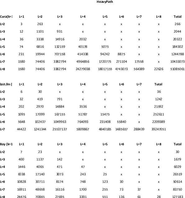

Our main result is that HeavyPath is algorithmically superior to all compared algorithms including Rank Join, in terms of the amount of work done. We establish this claim in multiple levels, by performing additional experiments that include comparing the number of edges read, the paths created, and the rate at which the thresholds decay. In all these experiments, we set , i.e., we focused on the top path.
Edge Reads. We measured the total number of edge reads performed by HeavyPath and by NextHeavyPath, where every time an edge is read, under sorted or random access or while performing joins to construct paths, is counted as one. We show the results in Figure . The # edge reads for NextHeavyPath exceeds for path lengths beyond 4 on Cora and last.fm and beyond 11 on Bay, which then runs out of memory. On the other hand, HeavyPath is able to go up to lengths 8, 7, and 36 on the three respective data sets, incurring far fewer edge reads. The reason for running out of memory has to do with the number of paths computed and examined, investigated next.
Paths Constructed. We counted the number of paths. In case of Rank Join, we only counted paths of length where is the required path length. In case of HeavyPath, we counted paths of all lengths that are constructed and stored by it in its buffers. The results are shown in Figure . The relative performance of HeavyPath and Rank Join w.r.t. the number of paths computed by them is consistent with the trend observed in the previous experiment on # edge reads, showing HeavyPath ends up doing significantly less work than Rank Join and hence is able to scale to longer lengths.
Threshold Decay. Both algorithms rely on their stopping threshold, for Rank Join and for HeavyPath for early termination. We measured the rate at which the thresholds decay since that gives an indication how quickly the algorithm will terminate. Figure shows the results. For each algorithm, the threshold value is shown until the algorithm terminates, successfully finding the heaviest path. It is obvious that in all cases, the threshold of HeavyPath decays extremely fast, whereas in comparison, the threshold used by Rank Join decays much more slowly. Since HeavyPath employs random accesses whereas Rank Join doesn’t, it is clear that random access is responsible for the rapid decay of the threshold, resulting in significant gain in performance. Please notice, the three experiments above are absolutely unaffected by systems issues, including garbage collection.
Running time. Finally, we separated the total running time into time spent on garbage collection and the rest. Let’s call the rest “compute time” for convenience. We compare the total time for HeavyPath with the compute time for the other algorithms. It is worth noting here that for the majority of the points reported in our results (which of course correspond to those cases where the appropriate algorithm terminated) successfully, garbage collection time was either or very small. The result is shown in Figure . For simplicity, we “time out”, i.e., stop the experiment, whenever the time taken exceeds seconds. It can be observed that despite taking out the (small to negligible amount of) garbage collection from the total times of other algorithms, the total time of HeavyPath is still significantly less than the compute times of other algorithms.
In each of these experiments, we can observe that HeavyPath significantly outperforms other algorithms. These experiments clearly establish that HeavyPath’s superiority over the other algorithms in terms of the amount of work done, i.e., in purely algorithmic terms, regardless of systems issues, and that our findings are not in any way compromised by garbage collection.