A phenomenological theory of Eulerian and Lagrangian velocity fluctuations in turbulent flows
Abstract
A phenomenological theory of the fluctuations of velocity occurring in a fully developed homogeneous and isotropic turbulent flow is presented. The focus is made on the fluctuations of the spatial (Eulerian) and temporal (Lagrangian) velocity increments. The universal nature of the intermittency phenomenon as observed in experimental measurements and numerical simulations is shown to be fully taken into account by the multi scale picture proposed by the multifractal formalism, and its extensions to the dissipative scales and to the Lagrangian framework. The article is devoted to the presentation of these arguments and to their comparisons against empirical data. In particular, explicit predictions of the statistics, such as probability density functions and high order moments, of the velocity gradients and acceleration are derived. In the Eulerian framework, at a given Reynolds number, they are shown to depend on a single parameter function called the singularity spectrum and to a universal constant governing the transition between the inertial and dissipative ranges. The Lagrangian singularity spectrum compares well with its Eulerian counterpart by a transformation based on incompressibility, homogeneity and isotropy and the remaining constant is shown to be difficult to estimate on empirical data. It is finally underlined the limitations of the increment to quantify accurately the singular nature of Lagrangian velocity. This is confirmed using higher order increments unbiased by the presence of linear trends, as they are observed on velocity along a trajectory.
Résumé
Une théorie phénoménologique des fluctuations de vitesse Eulérienne et Lagrangienne dans un écoulement turbulent Nous présentons une théorie phénoménologique des fluctuations de vitesse dans un écoulement turbulent pleinement développé isotrope et homogène. Nous mettons l’accent sur les fluctuations des incréments spatiaux (Eulérien) et temporels (Lagrangien) de vitesse. La nature universelle du phénomène d’intermittence observé sur les mesures expérimentales et les simulations numériques est complètement pris en compte par les arguments développés par le formalisme multifractal, et ses extensions aux échelles dissipatives et au cadre Lagrangien. Cet article présente les prédictions de cette description multifractale et les compare aux données empiriques. En particulier, des prédictions explicites sont obtenues pour des grandeurs statistiques, comme les fonctions de densité de probabilité et les moments d’ordres supérieurs, des gradients de vitesse et de l’accélération. Dans le cadre Eulérien, à un nombre de Reynolds donné, nous montrons que ces prédictions ne dépendent que d’une fonction à paramètres, appelée spectre de singularités, et d’une constante régissant la transition entre les régimes inertiels et dissipatifs. Le spectre des singularités Lagrangien est relié à son homologue Eulérien par une transformation basée sur la nature incompressible, homogène et isotrope de l’écoulement, alors que la constante restante est difficile à estimer à partir des données. Nous montrons finalement que l’incrément est inadapté à quantifier précisément la nature singulière de la vitesse Lagrangienne. Cela est confirmé par l’utilisation d’incréments d’ordres supérieurs non biaisés par la présence de comportements linéaires, comme nous l’observons sur la vitesse le long d’une trajectoire. Pour citer cet article : L. Chevillard et al., C. R. Physique volume (année).
Mots-clés : Turbulence ; Intermittence ; Eulérien et Lagrangien
Keywords:
Turbulence; Intermittency; Eulerian and LagrangianReceived *****; accepted after revision +++++
1 Introduction
As a long-standing challenge in classical physics [1, 2, 3, 4, 5, 6, 7, 8, 9], fully developed turbulence is an archetypical non linear and non local phenomenon. When a flow is stirred at a large scale , typically the mesh size of a grid in a wind tunnel or the width of the blades in a von Karman washing machine, the input energy cascades towards the small scales without being dissipated according to the classical picture of Richardson and Kolmogorov [1, 2]. One of the most important objectives in turbulence research is to understand the processes that lead to this very peculiar cascading structure of energy. As far as we know, recent theoretical progress made in this long lasting field comes from the systematic analysis and description of empirical (experimental and numerical) velocity data.
The first experimental measurements of turbulent velocity were performed in the Eulerian framework and focussed on the longitudinal velocity profile. In this context, the Taylor hypothesis allowed to interpret the time dependence of the measurements obtained in a wind tunnel behind a grid or in an air jet as a spatial dependence [7]. These experiments gave access to the longitudinal velocity increments, i.e.
| (1) |
where u is the velocity vector and a vector of norm , and the respective structure functions are given by
| (2) |
For such flows, the Reynolds number defined as
| (3) |
where is a characteristic velocity at the so-called integral length scale and the kinematic viscosity, can be considered as very large compared to unity. At these high Reynolds numbers, Kolmogorov showed, in a first seminal article [2] using a dimensional analysis, that the second order structure function behaves as a power law, i.e.
| (4) |
where is the Kolmogorov constant of order unity [10, 11] and the averaged dissipation that will be properly defined latterly. Equivalently, the power spectrum, i.e. the Fourier Transform of the velocity autocorrelation function, follows the celebrated Kolmogorov law,
| (5) |
where the proportionality constant can be calculated [10, 11]. As stated by Kolmogorov himself [2], the laws predicted (Eqs. 4 and 5) are only valid in a range of scales, called the inertial range (or equivalently ) delimitated by the Kolmogorov length scale under which dissipative effects dominate the physics. These laws have been successfully compared to empirical data [7]. If velocity fluctuations were Gaussian, these predictions could be easily generalized to higher order structure functions. As observed experimentally, the probability density functions (PDFs) of velocity increments undergo a continuous shape deformation, starting from the integral length scale at which statistics can be considered as Gaussian, down to the dissipative scales where the PDF is highly non Gaussian [12, 13, 14]. This phenomenon is a manifestation of the intermittent nature of turbulence, as first underlined by Kolmogorov and Obukhov [15, 16]. We show in Fig. 1(a) the estimation of the PDFs of longitudinal velocity increments obtained in the giant wind tunnel of Modane [17] at a high Taylor-based Reynolds number (Eq. 26 provides a link between the large-scale Reynolds number and ). The curves are arbitraly shifted vertically for the sake of clarity. This continuous shape deformation of these PDFs motivated Castaing et al. to build a statistical description of these longitudinal velocity fluctuations [12]. Moreover, by a simple visual inspection, we can remark that the PDFs are not symmetric. This is related to the Skewness phenomenon associated with the mean energy transfer of energy towards the small scales that takes place in the inertial range. We will come back to this point latterly.
The first part of this article is devoted to review the predictions that can be made using both the so-called multifractal formalism [7] and the propagator approach [12]. This description, that will be shown to depend only on a parameter function and a universal constant (independent on the flow geometry and the Reynolds number), accurately reproduces the non Gaussian features formerly presented.

More recently, experimental [18, 19, 20, 21, 22, 23, 24, 25, 26, 27]) and numerical [21, 22, 24, 28, 29, 30] data have revealed a similar phenomenon in the Lagrangian framework (see recent review articles [31, 33, 34]). Lagrangian velocity is defined as the Eulerian velocity of a fluid particle at the position , initially at the position via the following identity
| (6) |
In this framework, the study of the Lagrangian velocity fluctuations focusses on the Lagrangian time increment defined as
| (7) |
with a component of the Lagrangian velocity vector v (Eq. 6). A similar dimensional analysis à la Kolmogorov would give a linear dependence of the second order structure function
| (8) |
where is the integral time scale and the respective Lagrangian Kolmogorov constant [40, 41]. This corresponds to a Lagrangian power spectrum of the form
| (9) |
Once again, these laws are valid only in the respective inertial range (or ). Unfortunately, these laws cannot be easily generalized to higher order structure functions because of the fundamental non Gaussian nature of the velocity fluctuations. We show in Fig. 1(b) the estimation of the experimental velocity increments PDFs at various scales obtained at ENS Lyon [21] and the acceleration PDF obtained at the university of Cornell [25]. Let us first remark that the acceleration can be seen as a Lagrangian velocity increment at a scale much smaller than the Kolmogorov dissipative time scale. Again we observe a continuous shape deformation from Gaussian statistics at large scale, to long-tail acceleration statistics at vanishing scale. This is again a manifestation of the intermittency phenomenon.
We will show in this article that a similar statistical description can be developed in a Lagrangian context. The free parameters are again the corresponding singularity spectrum and a constant, as in the Eulerian framework. The Lagrangian singularity spectrum will be shown consistent with the prediction derived from its Eulerian counterpart using a transformation, presented latterly.
This article is devoted to the presentation of a phenomenological theory of the statistics of the Eulerian and Lagrangian velocity increments, from the integral length scale (or from the integral time scale ), down to the far dissipative scales based on the so-called multifractal formalism [7]. In this approach, statistical properties in the inertial range are assumed and compared to empirical data. This includes the classical K41 predictions “” (Eq. 5) and “” (Eq. 9), but also the intermittent (or multifractal) corrections. From this descriptive analysis, we predict the statistical properties of the (Eulerian) velocity gradients and (Lagrangian) acceleration as functions of the Reynolds number and of the corresponding singularity spectra. In this sense, we can consider the multifractal formalism, properly generalized to the dissipative range, as a phenomenological theory, i.e. statistical properties are assumed in the inertial range (given some free parameters fully encoded in the so-called singularity spectrum), and are predicted in the dissipative range. This was already recognized in Ref. [35]. To this regard, multifractal formalism can be viewed as a standard model of turbulence, and, as far as we know, it is the only formalism able to reproduce accurately higher order statistics of velocity increments. The most important perspective would be to establish a link between this formalism (in particular the existence of a singularity spectrum) and the equations of motion (i.e. the Navier-Stokes equations). This is out of the scope of the present article. Let us also mention some alternative statistical formalisms that are able to reproduce the non-Gaussian nature of the underlying statistics, such as, among others, “superstatistics” [36], continuous-time random walk models [37], vortex filament calculations [38] and kinetic equations approach [39]. As an interesting application of this multifractal formalism, we reinterpret former measurements by the group of Tabeling [44, 45], concerning the velocity gradients flatness as a function of the Reynolds number. We end with a general discussion of the skewness phenomenon and of its implications on the modeling of velocity increments in the inertial range. In the Lagrangian framework, we introduce higher order velocity increments designed to quantify accurately the singular nature of velocity and justify their use.
2 The Eulerian longitudinal velocity fluctuations
2.1 Behavior of the flatness of velocity increments from experimental investigation

We show in Fig. 2 the estimation of the flatness of the longitudinal velocity increments in various flow configurations and various Reynolds numbers. The first set of data has been obtained in a Helium jet [46] at four different Reynolds numbers: , where the Taylor-based Reynolds number is proportional to the square-root of the large-scale Reynolds number (see Eq. 26). Also are displayed the results in an air jet experiment at the ENS Lyon at of C. Baudet and A. Naert. The higher Reynolds number () comes from the wind tunnel experiment in Modane [17]. For comparisons are also reported the results coming from a classical direct numerical simulation (DNS) of E. Lévêque [42] at a moderate Reynolds number based on grid points in a periodic domain.
The flatness as a function of the scale is represented in a logarithmic representation. Flatness is divided by 3, i.e. by the value of the flatness of a Gaussian random variable. The scales are renormalized by the length scale estimated such that the power-laws that are observed in the inertial range are indistinguishable. Then, is itself normalized by the Reynolds number, i.e. , where is a universal constant, that will be shown to be linked to the Kolmogorov constant (subsection 2.1.2). A similar procedure is applied to .
In this representation, the Kolmogorov length scale can be seen directly as . It delimits the inertial range, i.e. , and the dissipative range, i.e. .
2.1.1 The inertial range
Let us first focus on the inertial range. Over this range, we observe a universal (i.e. independent on both the Reynolds number and the flow geometry) power law of exponent . In the same range, the second order structure function behaves as a power law, i.e. (data not shown). Furthermore, we can see that the statistics at scales larger than the integral length scale are consistent with a Gaussian process since the Flatness is very close to 3. Indeed the flatness is slightly smaller than 3. This can be justified theoretically from PDF closures [47, 48]. We will neglect this effect in the sequel. At this stage, for , a probabilistic description of the velocity increments is straightforward, i.e. , where is a zero average unit variance Gaussian noise and , independent on the scale . Henceforth, the symbol stands for an equality in law, i.e. in probability. It means the the PDF and all the moments of the random variables on the two sides of the equality are equal.
In the inertial range, we need a probabilistic formulation of this power law behavior. This is clear at this stage that a simple Gaussian modeling is not enough since it would predict a scale-independent flatness of constant value 3. Furthermore, the parameters that we will use must be universal since the observed power-law is universal. The main idea to build up a probabilistic description is to mix Gaussian variables and, for example, to use a Gaussian random variable with a fluctuating variance. This was proposed in the so-called propagator approach [12]. The form of the fluctuations of this stochastic variance will be given by the standard arguments of the multifractal formalism [7]. The corresponding non-Gaussian modeling consists in writing:
| (10) |
with a fluctuating variable, independent on the unit-variance zero-average Gaussian noise , and characterized by its distribution function
| (11) |
In the limit of vanishing values of , and gain the mathematical status of the Hölder exponent and the singularity spectrum respectively. Let us stress that the -distribution (Eq. 11) is indeed normalized, and the range of integration [;] depends on the precise shape of the singularity spectrum. One of the main hypothesis of the multifractal formalism is to assume that is independent on the scale [7]. In this case, assuming , a steepest-descent calculation (see Appendix A) shows that (recall that and are assumed independent)
| (12) |
where and is the Gamma function. Hence, the form of the density (Eq. 11) implies that the structure functions behave as power-laws, with a set of exponents linked to via a Legendre transform [7]
| (13) |
It gives in a straightforward manner the behavior of the flatness in the inertial range, i.e. . Let us first mention that in a K41 framework, without any intermittency corrections, the singularity spectrum is equal to and for . In this case, using Eq. 13, we can easily show that , and because of the linearity of the function, the flatness is independent on the scale . Clearly, the universal power-law behavior of the flatness in the inertial range as shown in Fig. 2, is the signature of the presence of intermittency in turbulence.
In the literature, several models for have been proposed. One of the most widely used is the lognormal approximation, giving the simplest quadratic form of the spectrum including intermittency corrections, as proposed by Kolmogorov and Oboukhov [15, 16]:
| (14) |
In this case, the proposed stochastic modeling of the velocity increments (Eq. 10) has a simple probabilistic interpretation: with and , the velocity increments are modeled as a Gaussian noise multiplied by a lognormal multiplicator . This was the proposition made in the propagator approach [12]. It is easily seen that , leading to . In the sequel, we will choose and because (i) a numerical integration of Eq. 12 shows no difference with the indefinite case, (ii) as we will see, the extension to the dissipative range implies (see section 2.1.2) and (iii) rigorously, only Hölder exponents greater than 0 and smaller than 1 are accessible when using increments. Experimental and numerical data as displayed in Fig. 2 show that the flatness behaves as a universal power-law of exponent . This corresponds to , and is called the intermittency coefficient. Also seen on empirical data (data not shown), [49]. Thus, in the sequel, we will take , very close to its K41 prediction . This defines completely the quadratic singularity spectrum (Eq. 14).
Another widely used singularity spectrum is the She-Lévêque spectrum [50],
| (15) |
This spectrum is based on log-Poisson statistics [51] and yields . This implies that , a power-law behavior in good agreement with the empirical data shown in Fig. 2. More sophisticated methods based on wavelets [52, 53] agree on the difficulty to discriminate between log-normal and log-Poisson statistics, and none of these approximations, for the moment, have been derived rigorously from first principles (i.e. the Navier-Stokes equations). For these reasons, we will use, in the sequel, the simplest lognormal approximation (Eq. 14) that compares well with empirical data, at least for low order moments with and that gives a Gaussian distribution for the -exponent, that is easy to manipulate (see in particular in the stochastic modeling proposed in section 2.2.3).
Finally, the proposed stochastic modeling (Eqs. 10 and 11) includes a functional form for the probability density functions of the velocity increments. A formal derivation of these PDFs, starting from the product of two independent random variables is reported in Appendix B. In simple words, we can see that the random variable (Eq. 10) is fully defined when is given the law of (Eq. 11) and (let us say ), that we assume, at this stage, independent. To simplify the derivation of the PDF of (see Appendix B for a more rigorous derivation), let us consider only the absolute value of the velocity increment. We get
Given that the random variables and are independent, the PDF of is the convolution product of the PDFs of and , as it was noticed in Ref. [12], namely
Noticing that and , we finally get
| (16) |
which shows the expression of the PDF of the absolute value of the velocity increment. Without further assumptions, this derivation cannot be generalized to derive the PDF of the signed velocity increment, since we are taking at one point a logarithm, but it clarifies the fact that defining in probability a random variable (such as in Eq. 10) allows to derive the associated PDF.
Actually, Eq. 16 is also true for the signed velocity increment, as shown in Appendix B, and we get for the velocity increment PDF at the scale the following form:
| (17) |
where is the PDF of a unit-variance zero-mean Gaussian variable. A numerical investigation (data not shown) of the PDF (Eq. 17) shows the characteristic continuous shape deformation associated to the intermittency phenomenon, in a similar way than observed in Fig. 1(a). Once again, this PDF is symmetric, i.e. and thus fails to describe the skewness phenomenon. We invite the reader to have a look at the sections 2.2.1 and 2.2.3 that provide a formalism able to reproduce the asymmetry of the PDFs, as observed in empirical data. We will see in the following section how to introduce the dissipative effects in order to obtain predictions on the statistics of the velocity gradients.
2.1.2 The dissipative range
The flatness of velocity increments, shown in Fig. 2, behaves in a very different way in the dissipative range, i.e. for scales . First of all, no power-law is observed. Then, we can see a strong Reynolds-number dependence. This is very different from the behavior observed in the inertial range. In the limit of vanishing scales, the velocity increments can be Taylor expanded and we obtain , i.e. a linear behavior as a function of the scale. This implies that the flatness tends to a Reynolds-number dependent function, independent on the scale , i.e. . The aim of this section is to understand and model the transition from the observed power-law behavior of the flatness in the inertial range, to this scale-independent behavior in the dissipative range. But first of all, let us have a look at the empirical data.
In Fig. 2, we see that not all of the measurements exhibit at very small scales a scale-independent flatness. Only the DNS (), the air-jet () and the Helium-jet () have succedeed in resolving scales smaller than the Kolmogorov length scale. Indeed, the measurements are difficult because the Hot-wire size is usually of the order of the Kolmogorov length scale. If the Reynolds number is too high, dissipative scales are too small to be resolved (as for , and ). In the Modane’s wind tunnel, the integral length scale is very large, and despite the large Reynolds number (), should have been accessible (which is of the order of the millimeter). Unfortunately, the noisy local environment of the giant wind tunnel and the high temperatures reached ( Celsius) implied by the strong level of turbulence, prevented electronics from working properly at high frequency.
Given the experimental limitations, we see that the flatness underlies a rapid increase. This was the subject of Ref. [42]. The main underlying idea is the differential action of the viscosity. The multiplicator fluctuates in the inertial range. In the dissipative range, up to a (random) coefficient, the multiplicator becomes linear with respect to the scale in order to be consistent with the Taylor’s expansion. The viscosity will regularize this inertial-range singular behavior at a scale that depends on the strength of the singularity: the bigger is the multiplicator, corresponding to smaller -exponents, the smaller is the scale of regularization. Purely kinematic arguments, proposed in Ref. [42], show that the width of the so-called intermediate dissipative range [35], where and are respectively the smallest and biggest dissipative scales, indeed depends weakly on the Reynolds number
| (18) |
the Kolmogorov length scale lying in between. In the representation chosen in Fig. 2, this prediction (Eq. 18) implies that the observed rapid increase occuring in the intermediate dissipative range should be steeper and steeper as the Reynolds number increases. This is what is qualitatively observed as long as experimental technics were able to reach these very small scales.
This can be fully modeled in the context of the multifractal formalism. To do so, one has to come up with a dissipative scale that depends explicitly on the strength of the multiplicator, or in a more straightforward manner, on the exponent . Paladin and Vulpiani [54] first proposed such a -dependent cut-off. Their reasoning was based on the local Reynolds number. For a scale lying in the inertial range, a fluctuating Reynolds number can be defined using a fluctuating characteristic velocity , leading to the local Reynolds number . We can see that at the integral length scale, the associated Reynolds number is unique, does not fluctuate, and is given by . This allows to define unambiguously a dissipative length scale: a scale at which the local Reynolds number is of order unity . The order one constant , is a free parameter of the formalism, a priori universal. It has been introduced phenomenologically in Refs. [46, 55, 56]. We will take it to be and we will show that it is related to the Kolmogorov constant . From there, one obtains directly the main result of Ref. [54], namely
| (19) |
Based on this result, Nelkin [57] showed the implication of a fluctuating dissipative scale (Eq. 19) on the modeling of the velocity increments for scales lying in the dissipative range. Within our approach summarized by Eq. 10, the velocity increment at a scale smaller than the dissipative scale will be modeled in the following way:
| (20) |
where , as in Eq. 10, is a zero-mean unit variance Gaussian random variable, , independent of the random exponent . This probabilistic modeling (Eq. 20) is consistent with the Taylor expansion of the velocity increment. It implies a model for the velocity gradient [57], namely:
| (21) |
Also we see that the proposed modeling for (Eq. 10) and for (Eq. 20) is continuous at the dissipative length scale .
As in Eqs. 10 and 11, to fully characterize in a probabilistic manner the random variable (Eq. 20), we need to define the distribution of the exponent . The proposition of Ref. [57] is to take for the distribution of at the dissipative scales a scale-independent distribution (up to a normalizing function ) that also has to be continuous at the transition , namely
| (22) |
where is the same universal function entering in the -distribution of the inertial range (Eq. 11), that we will approximate to be quadratic (Eq. 14).
As a general remark, as previously underlined in Ref. [35], the multifractal formalism becomes predictive. Indeed, given the description of the inertial range (Eqs. 10 and 11), and in particular given the singularity spectrum , we can predict the behavior of the velocity increments in the dissipative range (Eqs. 20 and 22) by a simple continuity argument. As a consequence, using Eqs. 19, 21, and 22, the -order moment of the velocity gradients is given by following function of the Reynolds number:
| (23) |
where , and . The distribution of a Gaussian variable is even, so all the odd moments of both velocity increments (Eqs. 10, 20) and gradients (Eq. 21) are vanishing at this stage. To include the skewness phenomenon, that requires further probabilistic modeling, we invite the reader to take a look at section 2.2.1.
The explicit form of even-order moments of velocity gradients (Eq. (23)) allows us to derive two important predictions: the computation of the average dissipation and the dependence on the Reynolds number of the flatness of the velocity derivatives. The dissipation is a key quantity in turbulence theory [7]. In an isotropic and homogeneous flow, the average dissipation is related to the second order moment of the velocity gradients as . Using Eq. (23), one obtains
| (24) |
In the limit of large Reynolds number, a steepest-descent calculation (see Appendix A) shows that, up to an order one multiplicative constant, the former integral, is dominated by the term , where . Because by construction, and for a wide class of singularity spectrum such that (via a Legendre transform, c.f. Eq. 13) , which is the case with the quadratic approximation (Eq. 14) with , we can show [7] that . This implies that is independent on the Reynolds number. This verifies a basic hypothesis of Kolmogorov, namely the finiteness of at infinite Reynolds number. A precise estimation of the integrals entering in Eq. 24 (see Appendix A) shows that
| (25) |
As shown in Refs. [42, 43], Eq. 25 gives a prediction of the Kolmogorov constant . Indeed, in the inertial range, neglecting intermittent corrections, the structure function is given by . Using Eq. 25, it gives , showing indeed that this constant is related to the Kolmogorov constant . Using , one finds , which is slightly bigger than what has be measured on empirical data [10, 11]. One of the reasons of this apparent discrepancy is related to the fact that the constant is clearly linked to the presence of intermittency and the implied extension of the intermediate dissipative range, whereas the definition of the assumes the absence of intermittency corrections. The prediction of the second order moment of the gradients allows also to link precisely the (large-scale) Reynolds number to the Taylor based Reynolds number in the following way:
| (26) |
Another important prediction is the dependence of the flatness of derivatives on the Reynolds number [57]. From Eq. 23, using a steepest-descent argument, we can show that, up to multiplicative constants of order unity (given in Appendix A):
| (27) |
Using the quadratic spectrum (Eq. 14), , and Eq. 26 for the Taylor-based Reynolds number dependence, we obtain:
| (28) |
which is consistent with empirical observations [58, 59, 60, 61]. More precisely, we compare in Fig. 3 the multifractal prediction (Eq. 28) with various experimental measurements and numerical simulations as compiled in Ref. [61]. The present theoretical prediction reproduces quantitatively the empirical observations. Let us stress that the quantitative dependence of the flatness of velocity derivatives on the Reynolds number (Eq. 28) is a genuine consequence of the intermittent nature of turbulence. In a K41 framework, this quantity would be Reynolds number independent.
2.1.3 Full multi scale description

In the preceding sections (2.1.1 and 2.1.2), we have seen how to model velocity fluctuations in respectively the inertial and far-dissipative ranges. It remains to write down a formalism, based on these two well known limiting ranges, that reproduces velocity statistics in the entire range of scales, including the intermediate dissipative range.
A first naive idea to gather both the inertial and dissipative ranges in a unified description is to consider, at a given scale and Reynolds number , the -exponents. Within the range , if , then the velocity increment lies in the inertial range; On the opposite, if , then the velocity increment lies in the dissipative range. The transition occurs at the exponent defined by , namely
| (29) |
Using both the laws of the velocity increments in the inertial (Eqs. 10 and 11) and dissipative (Eqs. 20 and 22) ranges, we then obtain
| (30) |
where normalizes the probability densities, namely
| (31) |
Unfortunately, this model does not compare well with empirical data because the transition is too sharp (data not shown, see [63]). Furthermore, the present modeling gives a continuous but not differentiable modeling of the velocity increment.
A continuous and differentiable transition, inspired by the interpolation function of Batchelor to model the second-order structure function [65], has been proposed in Ref. [64] as the entire range of scales. In Ref. [43], a slight modification of the proposition of Ref. [64] has been introduced in order to make the transition compatible with the far-dissipative predictions of Ref. [57]. It reads
| (32) |
where the random variable is again a zero-mean unit-variance Gaussian noise, , and
| (33) |
The normalizing constant is again such that , namely
| (34) |
Note that at a fixed given scale , the velocity increment (Eq. 32) and the -distribution (Eq. 33) tend to the inertial description (given by Eqs. 10 and 11) in the limit of infinite Reynolds number. In the same manner, at a given finite Reynolds number, this proposed description tends to the dissipative predictions (Eqs. 20 and 22)) in the limit of vanishing scales .
We show in Fig. 3(a) the theoretical predictions of the flatness as a function of the scales for the different Reynolds numbers previously investigated in Fig. 2. To do so, we integrated numerically Eqs. 32 and 33 using a quadratic singularity spectrum, with and , and and . The Reynolds number is obtained from the Taylor-based Reynolds number using Eq. 26. The proposed description based on Eqs. 32 and 33, reproduces the main characteristics shown in Fig. 2, namely, the universal power-law behavior in the inertial range and the rapid increase of the flatness in the dissipative range. Obviously, the theoretical predictions do not suffer from a lack of resolution and so with the proposed renormalization of the scales and of the flatness, all the curves tend to a universal plateau given by Eq. 28 when . The rapid increase that takes place in the intermediate dissipative range is consistent with the kinematic prediction given in Eq. 18, namely the slope of this increase behaves as in this representation. We can see indeed that the higher is the Reynolds number, the steepest is the increase.
2.1.4 Reinterpretation of the Tabeling’s data as a non trivial effect of the dissipative physics

As an example of the implications of the present theory, we reexamine in this section the observations of Tabeling and Willaime [45]. These authors investigated fully developed turbulence in a Von-Karman flow in gazeous helium at low temperature. Varying the pressure of the gas, they could span an unusually large range of Taylor scale based Reynolds numbers . They measured the local velocity using a hot wire probe. Through the Taylor “frozen turbulence” hypothesis, they could access to the longitudinal derivative of the velocity, and its flatness (Eq. 28). Up to , their results are in good agreement with previous literature and the present prediction (Eq. 28). Surprisingly, at , presents a maximum, and goes down up to , then raises again slowly (Fig. 4).Tabeling and Willaime interpreted their results as some evidence of a transition in turbulent flows. Some comments suggested that this behavior of could be due to the finite size of the probe. However, as remarked by Tabeling and Willaime, this size (about 10m) is much smaller than the Kolmogorov dissipation length at . Moreover, such a limitation was expected to yield a saturation of at a constant value, not a well pronounced maximum.
Indeed, following the present multifractal theory, identifying the “velocity derivative” with a finite difference at a constant length gives a maximum for the flatness as shown in Fig. 4. This is due to the rapid rise of the longitudinal velocity difference flatness in the intermediate dissipative range. This maximum occurs when the length coincides with the lowest scale of this intermediate range, which is much smaller than . Using Eqs. 32 and 33 with a quadratic singularity spectrum (Eq. 14), , stars in Fig. (4) show the behavior predicted for if , in reasonable agreement with the size of the sensor.
However, the present theory cannot predict a further rise of as observed experimentally. Also, the width of the predicted peak is much wider than observed. The present theory can explain some of the surprising features observed, not all.
2.2 Consistent description of the skewness phenomenon
2.2.1 General discussion on the skewness phenomenon
This section is devoted to the modeling of the skewness of the velocity increments. As we just saw, modeling the velocity increment as a Gaussian random variable multiplied by a random amplitude (see Eq. 32) cannot reproduce the asymmetric nature of the distribution of velocity increments since the Gaussian random variable , and its independence on the amplitude lead to vanishing odd-order moments, i.e. , . Nevertheless, keeping the same probabilistic description as in Eqs. 32 and 33 for the second order moment of velocity increments, allows us to predict in a consistent way the third-order moment of velocity increments if we use the Karman-Howarth-Kolmogorov equation:
| (35) |
In Ref. [43] (see also Ref. [66]), we compared experimental data to the predictions obtained for using the Karman-Howarth-Kolmogorov equation 35 and the second order structure function obtained from Eqs. 32 and 33. Predictions and emprical data compares well in the whole range of scales [43] without additional free parameters. In particular, the level of skewness in the inertial range is well reproduced and can be shown to be related to the universal constant . If we neglect dissipative effects in the exact relation Eq. 35, and the intermittent corrections on the second order structure function, it is easy to see that is independent on the scale and can be further approximated to , in excellent agreement with empirical data [43]. Moreover, applying a Taylor development on both Eq. 35 and on the multifractal predictions (Eqs. 32 and 33) for the second order structure function, in the limit of vanishing scales, we get the following multifractal prediction for the third order moment of the derivatives:
| (36) |
where is a negligible additive term, coming from the Taylor’s development of the normalizing factor (Eq. 34) [43]. This prediction of the third order moment of the velocity gradient (Eq. 36) using a Batchelor-Meneveau type of transition between the inertial and dissipative ranges (Eqs. 32 and 33), depends on the singularity spectrum , measured in the inertial range on empirical data, and on the universal constant . We show in Fig. 3(d) the numerical estimation of the multifractal prediction of the Skewness of derivatives (using Eqs. 32, 33 and 36) as a function of the Taylor-based Reynolds number, using the quadratic singularity spectrum (Eq. 14) and . This prediction is compared to empirical data [60, 61, 62] as described in the figure caption and compiled in Ref. [61]. We observe some dispersion between the three different empirical skewnesses, although the dependence on the Reynolds number seems to be universal. The difference in amplitude could be due to a lack of experimental and numerical resolution, and/or to a lack of statistical convergence. Thus, if the multifractal approach fails to predict the value of the skewness, it does reproduce accurately the Reynolds number dependence. Indeed, using Eq. 36, a steepest-descent calculation shows that the skewness of the derivatives behaves as a power law of the Reynolds number, i.e.
| (37) |
with
| (38) |
Using a quadratic approximation for the parameter function (Eq. 14), we get . This power-law dependence on the Reynolds number has been already obtained by Nelkin [57] using a different, although related, approach based on the asymptotically exact relationship . As shown is Fig. 3(d), further numerical estimations of relation (36), once rephrased in terms of Taylor-based Reynolds numbers using Eq. 26, leads to the following dependence of the velocity derivative skewness on :
| (39) |
2.2.2 Modeling the velocity increments probability density function
Indeed, consistent predictions for higher odd order structure functions are needed to predict the shape of the full velocity increment probability density function (PDF). Several propositions were made in the literature to account for the asymmetry of the PDF linked to the skewness phenomenon [12, 43]. To do so, we must modify the noise entering in the probabilistic formulation Eq. 32, and/or correlate this noise with the exponent . Asymmetric PDFs can be obtained if we change the Gaussian random variable to a non-Gaussian noise, still independent on the scale and on the multiplicator . More precisely, it was proposed in Ref. [12] to consider the random variable as being a variable of density that now reads
| (40) |
where is a universal constant, independent on both Reynolds number and scales. The main problem using this peculiar noise (Eq. 40) is that it leads to non zero average velocity increments. This could be fixed by introducing a scale dependent free parameter that centers the whole velocity increment PDF. Furthermore, to reproduce the non trivial behavior of the skewness in the dissipative range, we need to modify the parameter , and to make it dependent on both scale and Reynolds number. In this spirit, still based on the hypothesis of independence of the two random variables and , a general development of the PDF of on a basis made of the successive derivatives of a Gaussian, called the Edgeworth’s development, was proposed in Ref. [43]:
| (41) |
where the coefficients are functions of the scale . As previously shown, the symmetric part (even terms) is well described by a Gaussian noise, which means that and for . The coefficient is set to zero since, from Eq. 41, . Under these hypotheses, the third order moment is then given by , which fully determines the coefficient thanks to the Karman-Howarth-Kolmogorov equation (Eq. 35). Importantly, does depend on scale and Reynolds number. As Eq. 35 is the only available constraint on , it is tempting (as a first approximation) to restrict the expansion to : for . Additional statistical equations involving higher order odd moments of would be needed to give the next . This would require further modeling (primarily to get ride of pressure terms), which is outside the scope of the present work. Unfortunately, this crude approximation for the odd terms leads to severe pathologies, such as negative probability for rare large events, and is not consistent with higher order statistics such as hyperskewness (data not shown). To remedy for this weakness, Ref. [43] proposed to modify the variance of the Gaussian associated to the third term in the development (Eq. 41), in the following way:
| (42) |
where is fully determined by the exact relation 35, and an add-hoc free parameter, close to unity [43], aimed at describing higher order odd statistics. Then, from Eqs. 32, 33 and 42, the velocity increment PDF can be written, under the hypothesis of independence of and as (see Appendix B):
| (43) |
Then, using a quadratic singularity spectrum (Eq. 14), and the add-hoc coefficient (see Ref. [43]), the predicted PDF (Eq. 42) successfully compares to empirical data [43] as shown in Fig. 1(a) for various scales. The shape of the experimental velocity increment PDFs, from the inertial, to the intermediate dissipative and far dissipative ranges is well captured by the present theoretical prediction (Eq. 42), consistently with the behaviors of the flatness and skewness of the velocity increments. Unfortunately, at this stage, it is not possible to motivate the choice of the additional free parameter . To avoid having recourse to this parameter, we are forced to abandon the hypothesis of independence of the singularity exponent and the noise . A formalism that takes into account possible correlations between these two random variables is presented in the following section.

2.2.3 Probabilistic modeling of the skewness in the inertial range
It remains to give a consistent description of the asymmetric part of velocity increment PDFs in both the inertial and dissipative ranges without invoking an additional free parameter in the PDF of the noise (Eq. 42). In this section, we propose such a formalism for the inertial range, and leave the extension to the dissipative range to future investigations. The main idea is to correlate the exponent and the noise in the multifractal description provided by Eq. 32.
Let us first assume that the velocity increment can be written as a product of a Gaussian noise and an amplitude : , as in Eq. 32. The main difference with former assumptions is to let possible a correlation between and . The simplest way to deal with such a probabilistic formalism is to assume and jointly Gaussian. In this case, see Appendix B, the velocity increment PDF can be written as
| (44) |
where is the joint probability of the random variables and given by:
| (45) |
In Eq. 45, and (resp. and ) stand for the mean and variance of the random variable (resp. ). The correlation coefficient lies in the range . At large scale one has to recover . This implies .
Consistently with Eqs. 11 and 14, the multifractal formalism sets the mean and variance of the random variable to:
| (46) |
where remains the intermittency coefficient ( in empirical data, c.f. Fig. 2). Using the Legendre transform (Eq. 13), the -distribution leads to a set of structure function exponent
| (47) |
Using Eq. 44, we can show that
| (48) |
The velocity increment statistics are of zero-mean if and only if
| (49) |
For such parameters, we obtain the following velocity increment moments
| (50) |
The remaining free parameter is the correlation coefficient that will be fully determine by the Karman-Howarth-Kolmogorov equation (Eq. 35) and the Kolmogorov constant (or equivalently by ) . Indeed, neglecting dissipative effects, Eq. 35 gives . The average dissipation is given as , where (Eq. 25). Using the expression of given in Eq. 50, we obtain for , after solving a polynomial of third order, the following scale dependence
| (51) |
with
| (52) |
Using the scale dependence of the correlation coefficient (Eq. 51), we can see that the proposed description is consistent as long as the coefficient remains bounded in between -1 and 1. It corresponds to scales , using and . We finaly obtain for the Skewness and Flatness factors
| (53) |
We see that the proposed description (Eqs. 44 and 45), fully determined by the intermittent coefficient , the Karman-Howarth-Kolmogorov equation (Eq. 35, setting ) and the Kolmogorov constant (or equivalently ), gives consistent predictions (Eq. 53). Indeed, if intermittency is neglected, , the skewness is constant and compares well with empirical skewness in the inertial range [43]. Let us also notice that the flatness does not tend to its Gaussian value when , but to . This could be corrected if a large-scale cut-off is introduced in an ad-hoc way.
In Fig. 5 are shown the results of the numerical integration of Eqs. 44 and 45, using and . In Fig. 5(a) we recover the characteristic shape deformation of the velocity increments PDFs. In Fig. 5(b), the velocity increments Skewness and Flatness are estimated and compared succesfully to the analytical calculations given in Eq. 53. We also display in Fig. 5(c) and (d) the second and fourth order pre-multiplied PDFs. We can see that the core of velocity increments PDF dominates in the second pre-multiplied PDFs, whereas the tails of the velocity increments PDFs contribute significantly to the fourth-order one.
3 The Lagrangian framework
Recently, several experimental technics [18, 19, 20, 21, 22, 23, 24, 25, 26, 32, 27] and massive numerical computations [28, 21, 22, 24, 30, 32, 68] have been developed aiming following fluid particles along their trajectory in a fully developed turbulent flow. As stated in the introduction, a phenomenology similar to the Eulerian one can be developed in a Lagrangian context. The goal of this section is to present such a phenomenology introduced in Ref. [24], that has been compared to a compilation of empirical data in [24, 33].
3.1 Probabilistic formalism of the inertial and dissipative ranges
3.1.1 The inertial range
In the same spirit as in the section 2.1.1 devoted to the Eulerian framework, a probabilistic formulation of the Lagrangian velocity time fluctuations can be written down [24]. As observed experimentally, at the large integral time scale , related to the integral length scale , the statistics of both velocity increments and velocity are very close to Gaussian statistics. Indeed, in stationary, incompressible, homogeneous and isotropic turbulent flows, the Lagrangian velocity statistics can be related to their Eulerian counterparts [4] (see also Section 3.2.1). The statistics of the velocity time increments at a time scale (Eq. 7) can be modeled once again as the product of two independent random variables:
| (54) |
where is a zero-mean unit variance Gaussian random variable and . The exponent is independent on and fluctuates according to the distribution law:
| (55) |
where, according to the multifractal formalism assumptions, the Lagrangian singularity spectrum is universal (i.e. Reynolds number independent) and independent on the time scale . As with Eqs. 10, 11 and 13, this probabilistic modeling (Eqs. 54 and 55) is consistent with a power-law behavior of the Lagrangian structure functions , the exponents are related to the Lagrangian singularity spectrum via a Legendre transform:
| (56) |
Dimensional analysis (Eqs. 8 and 9) leads to a K41 description of Lagrangian turbulence neglecting intermittency. In this case, and for . Experimental and numerical data actually revealed the presence of intermittency [21, 24, 28, 30, 33] that can be characterized by a quadratic singularity spectrum [24]:
| (57) |
Note that the obtained value of is consistent with empirical data and with the dimensional prediction . As in the Eulerian framework, the bounds of the integration domain in Eq. 55 are and (see Section 4.1). We will see in the following (Section 3.3) that the quadratic approximation (Eq. 57) is too crude to describe the statistics of the acceleration and is not compatible with a quadratic Eulerian singularity spectrum via the Borgas’ transformation (see section 3.2). Nevertheless, it gives a consistent description of the Lagrangian velocity statistics in the inertial range as well as in the intermediate and far-dissipative range [24].
3.1.2 The dissipative range
As previously reported, the quadratic Eulerian spectrum (Eq. 14) has been extensively compared to a large set of empirical data, some of them displaying a large inertial range (in particular the Modane wind tunnel data, ). Sophisticated signal analysis procedures [53, 69] concluded that this quadratic approximation cannot be distinguished from the data and this for both the increasing part (positive order structure functions) and the decreasing part (negative order structure functions) of the spectrum. In the Lagrangian framework, such an analysis is much more difficult because the experimental technologies (silicon strip detectors [19], acoustic scatering [21], rapid cameras [26, 27], etc.) are not as efficient as a well known hot-wire probe under the Taylor’s hypothesis [7]. More fundamentaly, at a same Reynolds number, the width of the inertial range is much greater in the Eulerian framework than in the Lagrangian counterpart. Indeed, dimensional analysis predicts a Kolmogorov dissipative scale proportional to , and in turn .
Let us now adapt the arguments justifying a fluctuating dissipative length scale in Ref. [54] to the dissipative time scales [79]. A local Reynolds number can be defined as , where is a characteristic fluctuating velocity at the time scale . From Eq. 54, we obtain:
| (58) |
Reproducing the argumentation developed in Refs. [54, 79], a h-dependent dissipative time scale can be defined as the scale such that the local Reynolds number (Eq. 58) is of order unity: . A priori, the universal constant is different from the corresponding Eulerian one . We thus obtain [79],
| (59) |
If we neglect the intermittency corrections (in a K41 framework), then the exponent is unique, and we recover the Kolmogorov’s dimensional prediction
| (60) |
For a time scale smaller than the dissipative time scale , the velocity time increment can be Taylor expanded, i.e. , being the acceleration. Like for the Eulerian velocity increments (Eq. 20), we obtain the following stochastic modeling of the velocity time increments in the far dissipative range:
| (61) |
In analogy with the Eulerian framework (Eq. 22) [57, 79], the distribution of the -exponents does not depend on the scale (up to the normalizing function ) and is a function of the Reynolds number:
| (62) |
From Eqs. 59, 61 and 62, we can derive the expression of the high order moments of the acceleration, in the same way we derived the prediction of the moments of the velocity gradients in the Eulerian framework (Eq. 23):
| (63) |
where and . Let us stress that the acceleration odd-order moments are predicted to vanish: as observed in data. Finally, acceleration PDF can be expressed as a function of the singularity spectrum and the constant :
| (64) |
where . A detailed discussion of the Reynolds number dependence of acceleration variance and flatness is provided in section 3.3.
3.1.3 Full multi scale description
As in section 2.1.3, we need an interpolation formula linking the velocity increments statistics in the inertial (Eqs. 54 and 55) and dissipative (Eqs. 61 and 62) ranges. An adapted Batchelor-Meneveau form inspired from the Eulerian framework (Eqs. 32 and 33) was proposed in Ref. [24]:
| (65) |
where again the random variable is a Gaussian noise of zero-mean and unit-variance, and
| (66) |
with
| (67) |
As in Eq. 33, the normalizing function is determined by imposing . The free parameter entering in Eqs. 65 and 66 actually controls the transition from inertial to dissipative physics: the bigger is, the steeper the transition. In the sequel, we will use the Batchelor value , as in the Eulerian framework. Let us point out that we have found when dealing with experimental signals and focussing on the second order log-cumulant [24] whereas the value was used in Refs. [68, 33] to describe the logarithmic local slope. Following Appendix B, the velocity increment PDF then reads (Eqs. 65 and 66):
| (68) |
We show in Fig. 1(b) the numerical estimation of the Lagrangian velocity increment PDF (Eq. 68) at different scales using a quadratic singularity spectrum (Eq. 57) and for two Reynolds numbers corresponding to the two sets of experiments ( for the acoustic scattering measurements at the ENS Lyon [21] and [25] for the Cornell’s sillicon strip detectors). We can see that the multifractal model predictions for the PDFs compared well to both sets of experimental velocity measurements [24]. We have used , , and to describe ENS Lyon PDFs. For the Cornell acceleration data, we have used Eq. 68 with , , and . As far as ENS Lyon data are considered, to obtain these free parameters, we have fitted the second order cumulant, i.e. the variance of , over the whole range of scales (inertial and dissipative), , and assumed known, and defining and as the minimizers of the quadratic error of the theoretical and empirical second order cumulant [24]. We have further shown [24] that a similar fitting procedure on DNS Data () leads to and , a value of the transition parameter closer to its Eulerian counterpart (i.e. , Eqs. 32 and 33). The low value of the parameter found in experiments can be interpreted as resulting from a low-pass filtering induced by the finitesize of the particule tracers.
As for Cornell’s data, we did not use the true acceleration PDF (Eq. 64) because the measured flatness is much lower than (i) the one predicted by the present multifractal formalism and (ii) what is obtained in DNS (see the discussion in section 3.3). We chose in Ref. [24] to consider the Cornell’s PDF shown in Fig. 1(b) as a velocity increment PDF at a small time scale , corresponding to in units of the Kolmogorov’s dissipative time scale (Eq. 60). Then, the respective intermittency coefficient and are extracted from Cornell’s acceleration data while minimizing the quadratic error of the theoretical and experimental PDF.

In Fig. 6(a) is shown the behavior of the flatness of Lagrangian velocity time increments as a function of the scale , for various Reynolds numbers (from to ) and flow configurations (DNS and experimental von Karman flows), as previously done in the Eulerian framework (Fig. 2). As expected for scales greater than the integral time scale , the statistics of velocity increments are close to Gaussianity. This can be deduced from the Gaussianity of Eulerian velocity increments for , using an ergodicity argument (see section 3.2).
In the inertial range, for time scales in the range , an universal Reynolds-number independent behavior is observed. Recall that in the Lagrangian framework, at a given Reynolds number, the width of the inertial range is expected smaller than its Eulerian counterpart . Therefore, we may think that observing clear power-laws for Lagrangian velocity fluctuations asks for higher Reynolds number than in the Eulerian framework. Indeed, for the range of Reynolds number available, no clear power laws are observed. This is confirmed when we display in Fig. 6(c) the local logarithmic slope where no plateau is observed in the inertial range at any Reynolds number. Thus, as far as Flatness is concerned, no clear power laws are observed.
Scales correspond to the intermediate dissipative scales. Note that the extension of the intermediate dissipative range in the Lagrangian framework is much wider than in the Eulerian framework. This is related to the fact that, as we will see, Lagrangian velocity is more intermittent than the Eulerian one, implying stronger fluctuations of the local dissipative time scale defined in Eq. 59. In this range of scales, we can also notice a Reynolds number dependence, that could be interpreted, as previously done in the Eulerian framework (Section 2.1.2), as a direct consequence of the fluctuating nature of the dissipative time scale. When the scale tends to zero, we observe a saturation of the velocity increments flatness to the corresponding acceleration flatness. This representation shows clearly the Reynolds number dependence of the acceleration flatness that will be further discussed in Section 3.3.
As we see, estimating the intermittency coefficient is difficult since, contrary to the Eulerian framework, no strict power laws are observed. Nevertheless, using Eqs. 65 and 66, we can predict the behavior of Flatness over the entire range of scales, not only the inertial range. In Fig. 6(b), we compare the DNS data () against the proposed formalism (Eqs. 65 and 66), using a quadratic singularity spectrum , an intermittency coefficient (and ), the Batchelor value for the transition and . Thus, we find that Lagrangian turbulence is more intermittent than its Eulerian counterpart. The present formalism reproduces quantitatively the behavior of the flatness in the inertial and intermediate dissipative ranges. In the far-dissipative range (when ), this formalism seems to overpredict the value of the acceleration flatness (see the discussion in section 3.3). Given this limitation, the comparison between theory and empirical data is very satisfactory.
We can see that, even if no clear power laws are observed, the present formalism gives a realistic picture of the Flatness at any scale. We can also see that, even if the multifractal formalism assumes the existence of power-laws in the asymptotic limit of very high Reynolds numbers, the predicted Flatness does not exhibit a clear power law at the finite Reynolds numbers under investigation. This can be clearly seen in Fig. 6(d) where the predicted logarithmic local slopes of Flatness, for the various Reynolds numbers given in Fig. 6(a), are shown. Theoretically speaking, the fact that no power laws are obtained in the model is mostly related to the wide extension of the dissipative range implied by the strong level of intermittency that prevents from getting an extended inertial range. Another reason that explains why no clear inertial range power-laws are obtained in the model is that, for the largest scales of the inertial range for which the ratio cannot be considered as small, the steepest-descent calculation (Eq. 56), that predicts power-laws, is not a good approximation of Eqs. 65 and 66. To this regard, studying the behavior of structure functions in a relative way [30, 32, 33], in the spirit of the extended self similarity, allows to weaken large-scale anisotropic effects and shows more clearly power-law behaviors. Nevertheless, when working at a very high Reynolds number, the model indeed exhibits a clear power-law for the Flatness. This can been seen in Fig. 6(d) where we superimpose (solid line with no symbols), as an illustration, the predicted logarithmic local slope of Flatness for . We see indeed the presence of a plateau in the inertial range.
3.2 The Borgas’ argument: linking Eulerian and Lagrangian intermittencies
This section is devoted to establish a link between the Eulerian singularity spectrum and its Lagrangian counterpart [24]. We will mainly recall the work of Borgas [79] and invite the reader to have a look at this reference for a detailed derivation. An alternative dimensional derivation of an equivalent relationship has been also proposed in the literature [70]. Let us also mention more general arguments developed on kinematic bases [71, 72].
3.2.1 Ergodicity principle
Establishing a relationship between Eulerian and Lagrangian fluctuations requires as basic statement some principle of ergodicity. In simple words, we will admit that in an isotropic, homogeneous, incompressible and stationnary flow, the Eulerian average of a physical variable, obtained from summing up its realizations over space is equal to its Lagrangian average, obtained from summing up its values along the trajectory of a particle. This was first recognized and formalized by Tennekes and Lumley [4].
More formally, let us consider a one-point physical variable (e.g. velocity, dissipation, pressure and its derivatives, etc.) that does not depend on the scale. In the Eulerian framework, this variable depends on the spatial coordinates and time . In a Lagrangian description of the flow, this variable can be written as a function of the initial positions of the particles and time . The assumption of incompressibility allows the following relationship
| (69) |
that expresses the fact that an incompressible fluid continues to fill the box as it moves around [4]. The next step requires the assumptions of isotropy and homogenity. When ensemble averaging the equality, this expectation can be taken inside the integrals by linearity. Then, homogeneity and isotropy allow us to remove these expectations from these integrals because of the independence over the space. Thus we are left with
| (70) |
The particular case of the observables and was treated in Ref. [4]. The expectation of these variables are the characteristic function the Eulerian and Lagrangian velocities. The equality of these characteristic functions implies the equality of the distribution and of all the moments of each velocity components, namely , . As observed in data, the Eulerian velocity has statistics close to Gaussian, which implies from the ergodicity principle the Gaussianity of the Lagrangian velocity. This has been checked in experiments as well as in simulations (see the Gaussian values of the Eulerian and Lagrangian velocity increments flatness shown in respectively Figs. 2 and 6).
The idea of Borgas was to apply this ergodicity principle to the (scalar) observable dissipation , i.e. and , with as a main outcome the equality of the moments of the Eulerian dissipation and of the moments of the dissipation as seen by the particle along its trajectory. The next subsection is devoted to recall the Eulerian multifractal predictions for the moments of dissipation, and to extend these predictions to the Lagrangian framework [79].
3.2.2 Multifractal description of dissipation fluctuations
For the sake of completeness, we repeat here the arguments developed in Ref. [79]. Multifractal predictions have been historically developed [7, 15, 16, 76, 77, 78] for the coarse-grained dissipation over a ball of size centered on the position :
| (71) |
For a scale lying in the inertial range, a formalism similar to the one developed for the velocity increment can be written (Eqs. 10 and 11) using an exponent and a singularity spectrum . Using the notations of Ref. [79], we can write (equality in probability law), and the probability to get an exponent at scale being given by . When the scale enters the dissipative range, we must take into account the fluctuating nature of the dissipative scale (Eq. 19) parametrized by the exponent , i.e. . The choice of Borgas to apply the ergodicity principle to the dissipation was influenced by the fact that, in the limit of vanishing scales, the coarse-grained dissipation leads to predictions for the point wise moments of dissipation. We get, neglecting multiplicative (Reynolds number independent, but dependent) constants,
| (72) |
In a Lagrangian formulation, we will consider the average of dissipation during a time scale :
| (73) |
In a similar fashion as developed for the Eulerian description, the multifractal description of the statistical properties of can be written down using the exponent and the respective Lagrangian singularity spectrum [79], i.e. (equality in probability law) and the probability to get an exponent at scale being given by . When taking into account the fluctuating nature of the dissipative time scale , we get
| (74) |
Identifying the leading order Reynolds number power laws exponents entering in the Eulerian and Lagrangian predictions of the pointwise moments of dissipation (Eqs. 72 and 74), we get a relationship between the Eulerian and Lagrangian singularity spectra:
| (75) |
This relationship is the main result (Eq. 5.6) of Ref. [79].
3.2.3 Refined similarity hypotheses
To investigate the implications of the Borgas’ relationship between the singularity spectra of dissipation and the singularity spectra of velocity, we need to use a dictionnary [7] between the statistical properties of the coarse-grained dissipation and of the velocity increments. This is provided by the Refined Similarity Hypothesis (RSH) of Kolmogorov and Oboukhov [15, 16]. In the Eulerian framework in an -dimensional Euclidian space, this hypothesis reads:
| (76) |
Similarly, in the Lagrangian framework, the RSH hypothesis reads
| (77) |
Only recently the Lagrangian RSH hypothesis (Eq. 77) has been verified in numerical simulations [73, 74]. Using Eqs. 76 and 77 to reinterpret Eq. 75, we easily derive the following relationship between the Eulerian and Lagrangian velocity singularity spectra (with ) [24]:
| (78) |
This relation Eq. 78 can be inverted
| (79) |
To end this section, let us emphasize that the relation 78 is consistent with a non intermittent (K41) picture of turbulence. In this case, the Eulerian singularity spectrum is such that and if . Using relation 78, we obtain and if . This is consistent with and more generally with Eq. 77.

We represent in Fig. 7 various singularity spectra used in the present article, in both the Eulerian and Lagrangian framework, as it was done in Ref. [24, 63]. First of all, we display the Eulerian quadratic (Eq. 14) and the She-Lévêque (Eq. 15) singularity spectra using respectively a thick solid and dashed lines. One can see that the increasing part of the spectra superimposes on each others. It means that, in a purely inertial description of turbulence, the quadratic and She-Lévêque spectra are indistinguishable when using positive-order structure functions. The decreasing parts are distinct. More sophisticated signal analysis methods than computing velocity increment moments are required to investigate the decreasing part of the singularity spectra, such as the wavelet transform modulus maxima (WTMM) [52], the inverse structure functions method [80] or the wavelet leaders [53]. The conclusion of these investigations is that, given the statistical limitations and linearization effects, experimental signals are consistent with a quadratic singularity spectrum (Eq. 14) for both the increasing and decreasing parts.
We furthermore display on the same plot (Fig. 7) the three different singularity spectra we are using. This includes the quadratic Lagrangian spectrum (Eq. 57) represented using a thin dotted lines, and the transformed Eulerian spectra using the Borgas’ relation (Eq. 78) displayed using thin solid and dashed lines. One can see that the increasing parts coincide for the three cases, quantitative differences are shown concerning the decreasing part. Let us stress clearly that the Borgas’ relation being nonlinear, a quadratic spectrum in the Eulerian spectrum is transformed into a non quadratic spectrum in the Lagrangian framework. This explains why the thin dotted and solid lines are distinct. In the sequel, we will see that the decreasing part has a strong influence on the statistics of dissipative quantities in Lagrangian turbulence such as the acceleration flatness (see section 3.3), giving several arguments to discriminate these spectra when compared to empirical data. Another important remark can be made at this stage. The Borgas’ transformation (Eq. 78), given the Eulerian spectra formerly introduced, predicts the existence of -exponent greater than unity. This has strong implications on the singular nature of Lagrangian velocity fluctuations as quantified with velocity increments and the universal character of acceleration. We invite the reader to sections 4.1 and 4.2 for further discussions of this important point.
3.3 Prediction of the variance and flatness of acceleration
This section is devoted to the multifractal predictions of acceleration. We will mainly focus on the variance and on the flatness. The even order moments of acceleration are given by Eq. 63. Recall that by definition, we get for the acceleration variance:
| (80) |
Using a Gaussian approximation of the former integral (see Appendix A), we get
| (81) |
where
| (82) |
and is the -exponent for which is minimum (in the same spirit as it is presented for the Eulerian case in Appendix A). Once rephrased in terms of mean dissipation (using Eq. 25, we obtain ) and in terms of Taylor-based Reynolds number (using Eq. 26), we obtain
| (83) |
where is a remaining non-dimensional quantity that includes intermittent corrections, tabulated in various flow conditions in Refs. [20, 75]
| (84) |
When using the quadratic Lagrangian singularity spectrum (Eq. 57) with , we get:
| (85) |
Alternatively; when introducing the Eulerian quadratic spectrum (Eq. 14) into the Lagrangian frame using Eq. 78, and , we obtain:
| (86) |
A very similar result is obtained when plugging the Eulerian She-Lévêque spectrum (Eq. 15) into the Lagrangian frame using Eq. 78, and :
| (87) |
These three predictions show similar dependence on the Reynolds number [79], but the multiplicative pre factor depends strongly on the constant (Eq. 84) that is found itself strongly dependent on the shape of the singularity spectrum (see also the following discussion on the acceleration flatness). We show in Fig. 8(a) the Reynolds number dependence of the factor (Eq. 84) for the three different sets of singularity spectrum and constants (Eqs. 85, 86 and 87).

Similar predictions can be derived for the acceleration flatness. This study will underline the limitations of the quadratic Lagrangian singularity spectrum (Eq. 57), to describe the fluctuations of the velocity increments. The acceleration flatness can be expressed as the following function of the Reynolds number (Eq. 63)
| (88) |
The predictions of the acceleration flatnesses obtained by numerical integration of the integrals entering Eq. 88 are shown in Fig. 8(b). These predictions are compared to DNS data, the ones used in Fig. 6 and the ones provided in Ref. [61]. Some quantitative differences are observed for both the Reynolds number dependence and the multiplicative pre factor that depends strongly on the value of . An analytical expression of the flatness (Eq. 88) can be obtained once again using a Gaussian approximation (c.f. Appendix A):
| (89) |
where
| (90) |
and is defined in Eq. 82. The exponents control the Reynolds number dependence of the acceleration flatness. They depend only of the shape of the singularity spectrum . In contrast, the multiplicative pre factor depends on both the shape of and . When using the quadratic Lagrangian spectrum (Eq. 57) with , we get
| (91) |
When introducing the Eulerian quadratic spectrum (Eq. 14) into the Lagrangian framework using Eq. 78, and , we obtain
| (92) |
whereas for the Eulerian She-Lévêque spectrum (Eq. 15) and , we get
| (93) |
The three predictions (Eqs. 91, 92 and 93) we made using the three different sets of parameters ( and ) show different behaviors. First, we can see quantitative differences on the dependence on the Reynolds number. When compared to data, the quadratic Lagrangian singularity spectrum (Eq. 57) gives an exponent much bigger than for the two other parameter sets. This seems to be consistent with data only at the lowest Reynolds numbers, but not at the highest Reynolds numbers where the predicted exponent leads to some overestimate of the flatness. On the opposite, the quadratic Eulerian singularity spectrum (Eq. 14) and the log-Poisson one (Eq. 15), once re-expressed in the Lagrangian framework using the Borgas’ transformation (Eq. 78), give a Reynolds number dependence consistent with data, especially at high Reynolds numbers. Second, the multiplicative pre factors depend strongly on the the shape of the respective and on .
Let us stress that the analytical approximations given in Eqs. 91, 92 and 93 differ from a numerical estimation of the integrals entering in Eq. 88. In particular, when the quadratic Lagrangian spectrum is chosen, differences are quantitatively significant. This is clearly due to the range of integration that is finite in the numerical integration (i.e. and ) whereas it is assumed infinite (i.e. and ) in the Gaussian approximation in order to get simple analytical formula (thus avoiding any corrections given by the error function Erf). Let us point out that if we instead use (i) the range and is used when working with the Eulerian quadratic singularity spectrum further transformed using Eq. 75, and (ii) the range and when working with the She-Lévêque spectrum (Eq. 15), then the analytical predictions (Eqs. 92 and 93) are very close to the numerical estimations of Eq. 88. This underlines the limitations of the quadratic Lagrangian singularity spectrum (Eq. 57) to represent the statistics of acceleration. Indeed, additional analytical work shows that the exponent that minimizes the function (Eq. 82) and leads to (c.f. Eq. 90) is negative when using the quadratic Lagrangian singularity spectrum (Eq. 57). This would imply the existence of unphysical negative -exponents. This drawback does not exist when using the Eulerian quadratic (Eq. 14) or the She-Lévêque spectra (Eq. 15). Once again, this tells us that the quadratic Lagrangian singularity spectrum (Eq. 57) is not able to reproduce the acceleration statistics (see section 4.1 for more detailed discussion about the range of integration ).
4 Further discussions regarding the singular nature of velocity
4.1 Comments on the integration bounds and .
This section is devoted to present further discussions on the choice of the integration bounds that has been made to define the probabilistic models of Eulerian (c.f. Eqs. 32 and 33) and Lagrangian (c.f. Eqs. 65 and 66) velocity increments. This requires a clear definition of the Hölder exponents . Let us stress that the dissipative cut-offs, as given by the fluctuating dissipative length scale (Eq. 19) and by the fluctuating dissipative time scale (Eq. 59), imply that in the Eulerian frame and in the Lagrangian counterpart. In the sequel, we will consider only inertial range fluctuations because the mathematical theory of singularities is well established (see Ref. [52] and references therein). Our choice of the integration domain will be based on these considerations. In Ref. [68], in which only the She-Lévêque spectrum is considered, other choices have been made.
The Hölder exponent at a point of a singular signal (the Lagrangian velocity could be chosen without loss of generality) is defined as the biggest exponent such that it exists a polynomial of order and a positive constant C verifying
| (94) |
Let us stress that is the Taylor’s development of order of the signal and typically, . In other words, is the exponent that defines the first singular behavior entering in the Taylor development of in the neighborhood of :
| (95) |
where and a constant. This shows that the velocity increment is only sensitive to exponents because it is orthogonal to constants only. Thus, we chose for the Eulerian framework and when dealing with the quadratic spectrum (Eq. 14) and and when dealing with the She-Lévêque spectrum (Eq. 15). Similar choices have been made in the Lagrangian framework, namely and when dealing with the Lagrangian quadratic spectrum (Eq. 57) and the Eulerian quadratic spectrum (Eq. 14) once transformed in the Lagrangian frame using Borgas’ relation (Eq. 78), and when dealing with the She-Lévêque spectrum (Eq. 15) once reexpressed in the Lagrangian frame.
As far as the quadratic spectrum (Eq. 14) is considered, let us stress that the Eulerian predictions based on Eqs. 32 and 33 are similar if one uses and or and , the two values of such that . In the Lagrangian framework, considering the quadratic spectrum (Eq. 57), the predictions based on Eqs. 65 and 66 depend quantitatively on the range of integration. This is related to the fact that the decreasing part of the Lagrangian quadratic spectrum (Eq. 57) reaches the zero value at . This would strongly suggest the possible existence of -exponents greater than unity, exponents that cannot be measured with an increment, as explained at the beginning of this section. This is thus very tempting to study Lagrangian velocity fluctuations with multi scale objects orthogonal to polynomials as it may appear in the Taylor development (Eq. 95) if singularities are greater than unity. This is the subject of the following section in which higher order increments are considered, as they were in Refs. [24, 63, 81, 82].
4.2 Wavelet analysis of Eulerian and Lagrangian fluctuations.
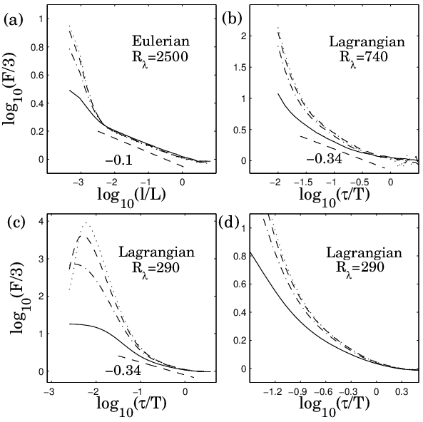
In order to check whether it exists singularities greater than unity, we perform a higher order increments study of velocity fluctuations. In the Eulerian framework, we will consider -order velocity increments defined as
| (96) |
With such defined velocity increments, singularities become accessible (see the discussion provided in section 4.1.
We display in Fig. 9(a) the results of the statistical analysis of the first four velocity increments on the experimental signal obtained in the Modane’s wind tunnel [17] that provides the highest Reynolds number . We choose to display only the velocity increment flatness defined as
| (97) |
In the inertial range of scales, namely , one can see that the observed power-law is independent on the increment order . This means that singularities greater than unity are not observed on Eulerian fluctuations, as it could have been expected from the shape of the well accepted quadratic or She-Lévêque singularity spectra. This has an important implication on the multifractal formalism: the Eulerian singularity spectrum is indeed measurable with the first order velocity increment.
At smaller scales lying in the dissipative range, one can see a quantitative dependence on the increment order : as increases, the transition from the inertial and dissipative ranges is steeper and steeper. This can be easily understood while generalizing the present probabilistic approach (Eqs. 32 and 33) to any -order velocity increments, with thus the same singularity spectrum . Indeed, the dependence on the order comes from the behavior in the dissipative range of the -order velocity increment, which, to be consistent with the Taylor development of velocity, reads
| (98) |
The fluctuating nature of the dissipative scale (Eq. 19) is independent on the way one is looking at velocity fluctuations and thus can be parametrized with the exponent , although the constant might depend on the order . The probabilistic modeling of velocity increments, consistent with the Taylor development 98, follows:
| (99) |
the random variable being again a zero average unit variance Gaussian noise, (this can be easily obtained using the binomial theorem), and the -distribution being unchanged an given by Eq. 33, but, in this case, and . A numerical investigation of the -order velocity increment flatness (Eq. 97) based on the proposed probabilistic modeling (Eqs. 99 and 33) shows the same type of behavior as observed on the Modane’s wind tunnel velocity data and depicted in Fig. 9(a), namely a -independent power-law in the inertial range and an intermediate dissipative steeper and steeper as the order increases (data not shown, see Ref. [63]). In the Eulerian framework, the first order increment allows to measure fully the singular nature of velocity, the -order increment appears as a tool that highlights unambiguously the dissipative range.
A similar study can be performed on the Lagrangian velocity using the -order velocity time increments defined in the following way:
| (100) |
We display the statistical analysis of the experimental measurements (in Fig. 9(b), ) and of the numerical simulations (in Fig. 9(c-d), ) of the Lagrangian velocity using the four first -order velocity time increments (Eq. 100). The results and interpretations are very different from the Eulerian case (presented in Fig. 9(a)). We can indeed see that, in the inertial range ( for the experimental signal and for the numerical simulation), the -order flatness underlies a transition between the and velocity time increment. Recall that in the Lagrangian framework, no clear power-laws are observed (see the discussion of Fig. 6). We display nevertheless the slope (i.e. ) that we would be observed if experimental data and simulations were performed at higher Reynolds numbers. As for velocity increments, higher order () velocity increments do not exhibit clear power laws but still do exhibit a steeper behavior. We are thus led to the conclusion that high order velocity increments do behave differently depending on the order : the level of intermittency for is lower than the one observed for . This can be seen as a proof of the existence of singularities greater than unity but smaller than 2, since the inertial range is found independent of the order as long as . It also says that the singular nature of Lagrangian velocity can be captured by an increment of order , the first order increment giving a biased singularity spectrum, that underestimates the intermittency coefficient, because of the existence of singularities greater than unity.
In the dissipative range, in a similar fashion than in the Eulerian case, the rapid increase of the flatness is steeper and steeper as the order of the analysing increment increases. This can be obtained using a similar probabilistic modeling of the velocity increment, as it was generalized in the Eulerian frame (i.e. Eq. 99):
| (101) |
the expressions of the dissipative time scale (Eq. 59) and the -distribution (Eq. 66) being unchanged, although the constant might depends on and the range of integration being and , and .
We have thus shown that some singularities exponent greater than unity and smaller than 2 exist in the Lagrangian frame, and not in the Eulerian frame. This observation is consistent with the Borgas’ transformation (Eq. 78) that indeed does predict these smooth behaviors in the Lagrangian trajectories starting from the well accepted Eulerian singularity spectra (Eqs. 14 and 15). This has a direct implication on the Lagrangian acceleration. Indeed, it suggests that acceleration might not be the right quantity to look at from a multi scale perspective. More precisely, it appears to be difficult to understand properly acceleration statistics as the dissipative limit of velocity increments statistics in the inertial range as it can be done in the Eulerian framework. This is also tempting to interpret the non universal features observed in empirical acceleration as a manifestation of the biased behavior of a first order increment and underlines the importance of Lagrangian velocity higher order derivatives as unbiased quantities.
5 Conclusions - Perspectives
We have shown all along the article that a phenomenological theory of turbulent velocity fluctuations can be written down. Assuming the probability laws in the inertial range, we can derive explicit predictions for the statistics of velocity gradients and acceleration that can be compared to experimental and numerical data. In the Eulerian framework, assuming a quadratic (Eq. 14) or a log-Poisson (Eq. 15) singularity spectra, and a universal constant , we can predict accurately the statistics of velocity gradients, including the flatness (Eq. 28) and skewness (Eq. 39).
In the Lagrangian framework, predictions, when compared to experimental and numerical data, are not as satisfactory as in the Eulerian framework. In particular, the remaing constant is shown to depend strongly on the precise shape of the Lagrangian singularity spectrum . Furthermore, it is shown, using the Borgas’ transform (Eq. 78), that the two widely accepted Eulerian singularity spectra (Eqs. 14 and 15) lead to quantitative differences when computing the acceleration flatness (Eqs. 92 and 93), whereas a quadratic approximation for (Eq. 57) leads to an irrealistic acceleration flatness (Eq. 91) at high Reynolds number. Nevertheless, these significant differences appear as a way to discriminate in the Eulerian framework the two former singularity spectra (Eqs. 14 and 15). We also mention the intrinsic limitations of the (first-order) velocity increment to quantify accurately the singular nature of the Lagrangian velocity (section 4.2). We thus propose to study higher order velocity increments (Eqs. 96 and 100) in order to quantify precisely the singular nature of the velocity fluctuations. We showed that indeed singularities greater than unity do exist in the Lagrangian framework.
As perspectives, we can mention:
- —
To investigate further the multifractal predictions of the velocity derivatives skewness (see section 2.2.1). The present formalism underestimates the skewness of derivatives when compared to data (see Fig. 3(d)), although the predicted Reynolds number dependence is realistic and a lot scatter is found in experimental data. To that regard, the experimental resolution is a key issue. Specially designed numerical experiments could give some hints on the influence of the resolution on this quantity, as it has been done in Ref. [83].
- —
A theoretical explanation of the value of the universal constant (or similarly of the Kolmogorov constant ) would be welcome. More precisely, we may wonder how this value depends on the shape of the singularity spectrum . This issue is even more crucial in the Lagrangian framework since (see section 3.3) the constant is very different if we work with different singularity spectra.
- —
We have seen that the (first-order) Lagrangian velocity increment is not adapted to study the singular nature of the velocity along the trajectories. The acceleration appears to be thus an ill-posed quantity and we could question its universality. Indeed, depending on the flow geometry (von Karman flow, wind tunnel, fully periodic DNS, etc.), a lot of scatter is found in data (see [75]). To this regard, the second-order time derivative of Lagrangian velocity may be more independent on the large scale geometry of the flow than the first-order one. Performing such a measurement (or a numerical simulation) will be much more difficult because of the presence of noise. It would be very interesting to quantify precisely the Reynolds number dependence of the variance and flatness of this quantity, as it was initiated in Ref. [61].
- —
The derivation of the Eulerian singularity spectrum from first principles is still missing. Recently, some progresses have been made while studying the dynamics of the velocity gradient tensor along Lagrangian trajectories [84, 86, 87, 85, 88, 89, 90, 91, 92]. In particular, in Refs. [90, 91] is proposed a stationary process for the velocity gradient tensor that predicts in a realistic way the longitudinal and transverse intermittencies. This theoretical investigation gives an Eulerian singularity spectrum consistent with the one observed on data (Eq. 14).
- —
In this article, we focus on two-points quantities, namely the velocity increments, fully determined by the corresponding probability densities and . Nothing is said on the long-range correlated nature of velocity. Indeed, it is shown in Refs. [22] and [25] that the acceleration amplitude is correlated over the integral time scale . In a similar fashion, it has been known for a long time that dissipation is correlated over the integral length scale [6, 93]. Taking into account this peculiar correlation structure of velocity allows to propose stochastic processes (one dimensional in the Lagrangian case, three dimensional vectorial for the Eulerian case) able to mimic the behavior of velocity in the inertial range [22, 94]. It remains to propose such stochastic processes able to reproduce velocity statistics in the intermediate and dissipative ranges and more generally, to give a stochastic representation of the differential action of viscosity as pointed out by the fluctuating nature of the dissipative scales (Eqs. 19 and 59).
Acknowledgements
We acknowledge for fruitfull discussions P. Abry, P. Borgnat, P. Flandrin. We thank Y. Gagne and the ONERA for providing the velocity signal of the wind tunnel of Modane, P. Tabeling and H. Willaime for the experimental data shown in Fig. 4, C. Baudet and A. Naert for the air-jet Eulerian data (), L. Biferale, A. Lanotte, F. Toschi for the Lagrangian numerical data ( shown in Fig. 6) and N. Mordant for Lagrangian experimental data ().
Appendix A Gaussian approximation and steepest-descent estimation
The aim of this Appendix is to elaborate on a Gaussian approximation that can be made to compute analytically the integrals entering, for example in Eqs. 24 or 28. Let us consider, without loss of generality, the integral
| (102) |
with . We first perform a Taylor’s development of the exponent of the Reynolds number around the exponent that minimizes it, namely
| (103) |
When assuming that and , we can approximate the integral as a Gaussian integral, i.e.
| (104) |
Then, the even order moment of velocity gradient (Eq. 23) can be obtained in the following approximate way (including the normalizing constant ):
| (105) |
Moreover from Eqs. 105 and 24, we get a precise estimation of the dissipation:
| (106) |
Using the quadratic singularity spectrum Eq. 14 with , we get
| (107) |
in very good agreement with the approximation made in Eq. 25. Similar calculations can be made for the velocity derivative flatness, and we get (for the quadratic singularity spectrum Eq. 14 with ):
| (108) |
once again is very close agreement with the approximation made in Eq. 28 without taking into account these corrections.
Appendix B Velocity increment and gradient probability density functions
We follow here the presentation of a classical textbook on random variables [67]. Consider two random variables x and y, and a function . We form the random variable z as a function of the two random variables x and y, namely
| (109) |
Consider the domain such that
| (110) |
The distribution function defined as the probability to have is given by [67]
| (111) |
where is the joint-density of the random variables x and y. Then, the probability density function is given by the derivative, with respect to , of the distribution function .
Consider now the random variable formed as the product of two random variables written as , with the function definite positive (Eqs. 32, 65 or 44). In this case, the domain is easily obtained
| (112) |
We get for the distribution function of the velocity increments
| (113) |
The probability density function of the random variable is readily obtained from Eq. 113 taking a derivative with respect to , and we get
| (114) |
which justifies Eq. 44. If furthermore, the random variables and are assumed independent, as in Eqs. 32 and 65, then the joint density can be factorized, i.e. and the distribution Eq. 43 is justified.
References
- [1] L. F. Richardson. Weather Prediction by Numerical Process, Cambridge University Press, Cambridge, 1922.
- [2] A. N. Kolmogorov, The local structure of turbulence in incompressible viscous fluid for very large Reynolds numbers, Dokl. Akad. Nauk SSSR 30 (1941) 301 [in Russian]. English translation: Proc. R. Soc. London, Ser. A 434 (1991), 9.
- [3] G. K. Batchelor, The Theory of Homogeneous Turbulence, Cambridge University Press, Cambridge, 1953.
- [4] H. Tennekes and J. L. Lumley, A First Course in Turbulence, MIT Press, Cambridge, MA, 1972.
- [5] R. H. Kraichnan, On Kolmogorov’s inertial-range theories, J. Fluid Mech. 62 (1974), 305.
- [6] A. S. Monin and A. M. Yaglom, Statistical Fluid Mechanics, MIT Press, Cambridge, MA, 1975.
- [7] U. Frisch, Turbulence, Cambridge University Press, Cambridge, 1995.
- [8] S. B. Pope, Turbulent Flows, Cambridge University Press, Cambridge, 2000.
- [9] A. Tsinober, An Informal Introduction to Turbulence, Kluwer Academic, Dordrecht, 2001.
- [10] P. K. Yeung and Y. Zhou, Universality of the Kolmogorov constant in numerical simulations of turbulence. Phys. Rev. E 56 (1997), 1746.
- [11] D. A. Donzis and K. R. Sreenivasan, The bottleneck effect and the Kolmogorov constant in isotropic turbulence, J. Fluid Mech. 657 (2010), 171.
- [12] B. Castaing, Y. Gagne and E. Hopfinger, Velocity probability density functions of high Reynolds number turbulence, Physica D 46 (1990), 177.
- [13] R. Benzi, L. Biferale, G. Paladin, A. Vulpiani, and M. Vergassola, Multifractality in the statistics of the velocity gradients in turbulence, Phys. Rev. Lett. 67 (1991), 2299.
- [14] P. Kailasnath, K. R. Sreenivasan, and G. Stolovitzky, Phys. Rev. Lett. 68 (1992), 2766.
- [15] A. M. Oboukhov, Some specific features of atmospheric turbulence, J. Fluid Mech. 13 (1962), 77.
- [16] A. N. Kolmogorov, A refinement of previous hypotheses concerning the local structure of turbulence in a viscous incompressible fluid at high Reynolds number, J. Fluid Mech. 13 (1962), 77.
- [17] H. Kahalerras, Y. Malécot, Y. Gagne, and B. Castaing, Intermittency and Reynolds number, Phys. Fluids 10 (1998), 910.
- [18] S. Ott and J. Mann, An experimental investigation of the relative diffusion of particle pairs in three-dimensional turbulent flow, J. Fluid Mech. 422 (2000), 207.
- [19] A. La Porta, G. A. Voth, A. M. Crawford, J. Alexander and E. Bodenschatz, Fluid particle accelerations in fully developed turbulence, Nature 409 (2001), 1017.
- [20] G. A. Voth. A. La Porta, A. Crawford, J. Alexander and E. Bodenschatz, Measurement of particle accelerations in fully developed turbulence, J. Fluid Mech. 469 (2002) 121.
- [21] N. Mordant, P. Metz, O. Michel, and J.-F. Pinton, Measurement of Lagrangian Velocity in Fully Developed Turbulence, Phys. Rev. Lett. 87 (2001), 214501.
- [22] N. Mordant, J. Delour, E. Lévêque, A. Arneodo, and J.-F. Pinton, Long Time Correlations in Lagrangian Dynamics: A Key to Intermittency in Turbulence, Phys. Rev. Lett. 89 (2002), 254502.
- [23] N. Mordant, J. Delour, E. Lévêque, O. Michel, A. Arneodo and J.-F. Pinton, Lagrangian Velocity Fluctuations in Fully Developed Turbulence: Scaling, Intermittency, and Dynamics, J. Stat. Phys. 113 (2003), 701.
- [24] L. Chevillard, S. G. Roux, E. Lévêque, N. Mordant, J.-F. Pinton, and A. Arneodo, Lagrangian Velocity Statistics in Turbulent Flows: Effects of Dissipation, Phys. Rev. Lett. 91 (2003), 214502.
- [25] N. Mordant, A. M. Crawford and E. Bodenschatz, Experimental Lagrangian acceleration probability density function measurement, Physica D 193 (2004), 245.
- [26] H. Xu, M. Bourgoin, N. T. Ouellette, and E. Bodenschatz, High order Lagrangian velocity statistics in turbulence, Phys. Rev. Lett. 96 (2006), 024503.
- [27] J. Berg, S. Ott, J. Mann, and B. Lüthi, Experimental investigation of Lagrangian structure functions in turbulence, Phys. Rev. E 80 (2009), 026316.
- [28] P. K. Yeung and S. B. Pope, Lagrangian statistics from direct numerical simulations of isotropic turbulence, J. Fluid Mech. 207 (1989), 531.
- [29] P. K. Yeung, Lagrangian characteristics of turbulence and scalar transport in direct numerical simulations, J. Fluid Mech. 427 (2001), 241.
- [30] L. Biferale, G. Boffetta, A. Celani, B. J. Devenish, A. Lanotte, and F. Toschi, Multifractal statistics of Lagrangian velocity and acceleration in turbulence, Phys. Rev. Lett. 93 (2004), 064502.
- [31] P. K. Yeung, Lagrangian investigations of turbulence, Ann. Rev. Fluid Mech. 34 (2002), 115.
- [32] L. Biferale, E. Bodenschatz, M. Cencini, A. S. Lanotte, N. T. Ouellette, F. Toschi, and H. Xu, Lagrangian structure functions in turbulence: A quantitative comparison between experiment and direct numerical simulation, Phys. Fluids 20, 065103 (2008).
- [33] A. Arneodo et al., Universal Intermittent Properties of Particle Trajectories in Highly Turbulent Flows, Phys. Rev. Lett. 100 (2008), 254504.
- [34] F. Toschi and E. Bodenschatz, Lagrangian properties of particles in turbulence, Ann. Rev. Fluid Mech. 41 (2009), 375.
- [35] U. Frisch and M. Vergassola, A prediction of the multifractal model: the intermediate dissipation range, Europhys. Lett. 14 (1991), 439.
- [36] C. Beck and E.G.D. Cohen, Superstatistics, Physics A 322, 267 (2003).
- [37] R. Friedrich, Statistics of Lagrangian Velocities in Turbulent Flows, Phys. Rev. Lett. 90, 084501 (2003).
- [38] K. P. Zybin and V. A. Sirota, Lagrangian and Eulerian Velocity Structure Functions in Hydrodynamic Turbulence, Phys. Rev. Lett. 104, 154501 (2010).
- [39] A. Daitche, R. Friedrich, O. Kamps, J. Llff, M. Voskuhle and M. Wilczek, The Lundgren-Monin-Novikov Hierarchy: Kinetic Equations for Turbulence, This specal issue of the Comptes Rendus de l’Académie des Sciences (2012).
- [40] S. Du, B. L. Sawford, J. D. Wilson, and D. J. Wilson, Estimation of the Kolmogorov constant (C0) for the Lagrangian structure function, using a second-order Lagrangian model of grid turbulence, Phys. Fluids 7 (1995), 3083.
- [41] R. Lien and E. D’Asaro, The Kolmogorov constant for the Lagrangian velocity spectrum and structure function, Phys. Fluids 14 (2002), 4456.
- [42] L. Chevillard, B. Castaing, and E. Lévêque, On the rapid increase of intermittency in the near-dissipation range of fully developed turbulence, Eur. Phys. J. B 45 (2005), 561.
- [43] L. Chevillard, B. Castaing, E. Lévêque, and A. Arneodo, Unified multifractal description of velocity increments statistics in turbulence: Intermittency and skewness, Physica D 218 (2006), 77.
- [44] P. Tabeling, G. Zocchi, F. Belin, J. Maurer, and H. Willaime, Probability density functions, skewness, and flatness in large Reynolds number turbulence, Phys. Rev. E 53 (1996), 1613.
- [45] P. Tabeling and H. Willaime, Transition at dissipative scales in large-Reynolds-number turbulence, Phys. Rev. E 65 (2002), 066301.
- [46] O. Chanal, B. Chabaud, B. Castaing and B. Hébral, Intermittency in a turbulent low temperature gaseous helium jet, Eur. Phys. J. B 17 (2000), 309.
- [47] M. Wilczek and R. Friedrich, Dynamical origins for non-Gaussian vorticity distributions in turbulent flows, Phys. Rev. E 80 (2009), 0160316.
- [48] M. Wilczek, A. Daitche and R. Friedrich, On the velocity distribution in homogeneous isotropic turbulence: correlations and deviations from Gaussianity, J. Fluid Mech. 676, 191 (2011).
- [49] A. Arneodo et al., Structure functions in turbulence, in various flow configurations, at Reynolds number between 30 and 5000, using extended self-similarity, Europhys. Lett. 34 (1996), 411.
- [50] Z.-S. She and E. Lévêque, Universal scaling laws in fully developed turbulence, Phys. Rev. Lett. 72 (1994), 336.
- [51] B. Dubrulle, Intermittency in fully developed turbulence: Log-Poisson statistics and generalized scale covariance, Phys. Rev. Lett. 73 (1994) 959.
- [52] J. F. Muzy, E. Bacry and A. Arneodo, Multifractal formalism for fractal signals: The structure-function approach versus the wavelet-transform modulus-maxima method, Phys. Rev. E 47 (1993), 875.
- [53] H. Wendt, P. Abry, and S. Jaffard, Bootstrap for empirical multifractal analysis, IEEE Signal Proc. Mag. 24 (2007) 38.
- [54] G. Paladin and A. Vulpiani, Degrees of freedom of turbulence, Phys. Rev. A 35 (1987), 1971.
- [55] Y. Malécot, C. Auriault, H. Kahalerras, Y. Gagne, O. Chanal, B. Chabaud, and B. Castaing, A statistical estimator of turbulence intermittency in physical and numerical experiments, Eur. Phys. J. B 16 (2000), 549.
- [56] Y. Gagne, B. Castaing, C. Baudet, and Y. Malécot, Reynolds dependence of third-order velocity structure functions, Phys. Fluids 16 (2004), 482.
- [57] M. Nelkin, Multifractal scaling of velocity derivatives in turbulence, Phys. Rev. A 42 (1990), 7226.
- [58] C. W. Van Atta and R. A. Antonia, Reynolds number dependence of skewness and flatness factors of turbulent velocity derivatives, Phys. Fluids 23 (1980), 252.
- [59] K. R. Sreenivasan and R. A. Antonia, The phenomenology of small-scale turbulence, Ann. Rev. Fluid Mech. 29 (1997) 435.
- [60] A. Gylfason, S. Ayyalasomayajula and Z. Warhaft, Intermittency, pressure and acceleration statistics from hot-wire measurements in wind-tunnel turbulence, J. Fluid Mech. 501 (2004), 213.
- [61] T. Ishihara, Y. Kaneda, M. Yokokawa, K. Itakura and A. Uno, Small-scale statistics in high-resolution direct numerical simulation of turbulence: Reynolds number dependence of one-point velocity gradient statistics, J. Fluid Mech. 592 (2007), 335.
- [62] R. Antonia, A. Chambers and B. Satyaprakash, Reynolds number dependence of high-order moments of the streamwise turbulent velocity derivative, Boundary Layer Met. 21 (1981) 159.
- [63] L. Chevillard, Unified Multifractal Description of the Intermittency Phenomenon in Eulerian and Lagrangian Turbulence, PhD Thesis, University of Bordeaux (2004), unpublished, can be found online at http://tel.archives-ouvertes.fr/.
- [64] C. Meneveau, Transition between viscous and inertial-range scaling of turbulence structure functions, Phys. Rev. E 54 (1996) 3657.
- [65] G. K. Batchelor, Pressure fluctuations in isotropic turbulence, Proc. Cambridge Philos. Soc. 47 (1951), 359.
- [66] W. Bos, L. Chevillard, J. Scott and R. Rubinstein, Reynolds number effect on the velocity increment skewness in isotropic turbulence, Phys. Fluids 24, 015108 (2012).
- [67] A. Papoulis, Probability, Random Variables and Stochastic Processes, McGraw-Hill Inc., New York, 1991.
- [68] R. Benzi, L. Biferale, R. Fisher, D.Q. Lamb and F. Toschi, Inertial range Eulerian and Lagrangian statistics from numerical simulations of isotropic turbulence, J. Fluid Mech. 653 (2010) 221.
- [69] J. Delour, J.-F. Muzy and A. Arneodo, Intermittency of 1D velocity spatial profiles in turbulence: a magnitude cumulant analysis, Eur. Phys. J. B 23 (2001), 243.
- [70] G. Boffetta, F. De Lillo and S. Musacchio, Lagrangian statistics and temporal intermittency in a shell model of turbulence, Phys. Rev. E 66 (2002), 066307.
- [71] H. Homann, O. Kamps, R. Friedrich and R. Grauer, Bridging from Eulerian to Lagrangian statistics in 3D hydro- and magnetohydrodynamic turbulent flows, New Journ. Phys. 11 (2009), 73020.
- [72] O. Kamps, R. Friedrich, and R. Grauer, Exact relation between Eulerian and Lagrangian velocity increment statistics, Phys. Rev. E 79 (2009), 066301.
- [73] R. Benzi, L. Biferale, E. Calzavarini, D. Lohse and F. Toschi, Velocity-gradient statistics along particle trajectories in turbulent flows: The refined similarity hypothesis in the Lagrangian frame, Phys. Rev. E 80 (2009), 066318.
- [74] H. Yu and C. Meneveau, Lagrangian refined Kolmogorov similarity hypothesis for gradient time evolution and correlation in Turbulent Flows, Phys. Rev. Lett. 104 (2010), 084502.
- [75] R.J. Hill, Scaling of acceleration in locally isotropic turbulence, J. Fluid Mech. 452 (2002), 361.
- [76] C. Meneveau, K.R. Sreenivasan, P. Kailasnath, and M. S. Fan, Joint multifractal measures: Theory and applications to turbulence, Phys. Rev. A 41 (1990), 894.
- [77] C. Meneveau and K. R. Sreenivasan, The multifractal nature of turbulent energy dissipation, J. Fluid Mech. 224 (1991), 429.
- [78] K. R. Sreenivasan and C. Meneveau, Singularities of the equations of fluid motion, Phys. Rev. A 38 (1988), 6287.
- [79] M. S. Borgas, The multifractal lagrangian nature of turbulence, Phil. Trans. R. Soc. Lond. A 342 (1993), 379.
- [80] L. Biferale, M. Cencini, D. Vergni, and A. Vulpiani, Exit time of turbulent signals: A way to detect the intermediate dissipative range, Phys. Rev. E 60 (1999), R6295.
- [81] E. Falcon, S. Fauve and C. Laroche, Observation of intermittency in wave turbulence, Phys. Rev. Lett. 98 (2007), 154501.
- [82] E. Falcon, S. Roux and C. Laroche, On the origin of intermittency in wave turbulence, Europhys. Lett. 90 (2010), 34005.
- [83] J. Schumacher, Sub-Kolmogorov-scale fluctuations in fluid turbulence, Europhys. Lett. 80 (2007), 54001.
- [84] P. Vieillefosse, Internal motion of a small element of fluid in an inviscid flow, Physica A 125 (1984), 150.
- [85] B. J. Cantwell, Exact solution of a restricted Euler equation for the velocity gradient tensor, Phys. Fluids A 4 (1992), 782.
- [86] W. T. Ashurst, A. R. Kerstein, R. M. Kerr, and C. H. Gibson, Alignment of vorticity and scalar gradient with strain rate in simulated Navier–Stokes turbulence, Phys. Fluids 30 (1987), 2343.
- [87] S. S. Girimaji and S. B. Pope, A diffusion model for velocity gradients in turbulence, Phys. Fluids A 2 (1990), 242.
- [88] M. Chertkov, A. Pumir, and B. I. Shraiman, Lagrangian tetrad dynamics and the phenomenology of turbulence, Phys. Fluids 11 (1999), 2394.
- [89] E. Jeong and S. S. Girimaji, Velocity-gradient dynamics in turbulence: Effect of viscosity and forcing, Theor. Comput. Fluid Dyn. 16 (2003), 421.
- [90] L. Chevillard and C. Meneveau, Lagrangian dynamics and statistical geometric structure of turbulence, Phys. Rev. Lett. 97 (2006), 174501.
- [91] L. Chevillard and C. Meneveau, Intermittency and universality in a Lagrangian model of velocity gradients in three-dimensional turbulence, C. R. Mec. 335 (2007), 187.
- [92] C. Meneveau, Lagrangian dynamics and models of the velocity gradient tensor in turbulent flows, Annual Rev. Fluid Mech. 43, 219 (2011).
- [93] R. A. Antonia, N. Phan‐Thien, and B. R. Satyaprakash, Autocorrelation and spectrum of dissipation fluctuations in a turbulent jet, Phys. Fluids 24 (1981), 554.
- [94] L. Chevillard, R. Robert and V. Vargas, A stochastic representation of the local structure of turbulence, Europhys. Lett. 89 (2010), 54002.