Asymptotically Exact Inference in Conditional Moment Inequality Models
Abstract
This paper derives the rate of convergence and asymptotic distribution for a class of Kolmogorov-Smirnov style test statistics for conditional moment inequality models for parameters on the boundary of the identified set under general conditions. In contrast to other moment inequality settings, the rate of convergence is faster than root-, and the asymptotic distribution depends entirely on nonbinding moments. The results require the development of new techniques that draw a connection between moment selection, irregular identification, bandwidth selection and nonstandard M-estimation. Using these results, I propose tests that are more powerful than existing approaches for choosing critical values for this test statistic. I quantify the power improvement by showing that the new tests can detect alternatives that converge to points on the identified set at a faster rate than those detected by existing approaches. A monte carlo study confirms that the tests and the asymptotic approximations they use perform well in finite samples. In an application to a regression of prescription drug expenditures on income with interval data from the Health and Retirement Study, confidence regions based on the new tests are substantially tighter than those based on existing methods.
JOB MARKET PAPER
1 Introduction
Theoretical restrictions used for estimation of economic models often take the form of moment inequalities. Examples include models of consumer demand and strategic interactions between firms, bounds on treatment effects using instrumental variables restrictions, and various forms of censored and missing data (see, among many others, Manski, 1990; Manski and Tamer, 2002; Pakes, Porter, Ho, and Ishii, 2006; Ciliberto and Tamer, 2009; Chetty, 2010, and papers cited therein). For these models, the restriction often takes the form of moment inequalities conditional on some observed variable. That is, given a sample , we are interested in testing a null hypothesis of the form with probability one, where the inequality is taken elementwise if is a vector. Here, is a known function of an observed random variable , which may include , and a parameter , and the moment inequality defines the identified set of parameter values that cannot be ruled out by the data and the restrictions of the model.
In this paper, I consider inference in models defined by conditional moment inequalities. I focus on test statistics that exploit the equivalence between the null hypothesis almost surely and for all . Thus, we can use , or the infimum of some weighted version of the unconditional moments indexed by . Following the terminology commonly used in the literature, I refer to these as Kolmogorov-Smirnov (KS) style test statistics. The main contribution of this paper is to derive the rate of convergence and asymptotic distribution of this test statistic for parameters on the boundary of the identified set under a general set of conditions. The asymptotic distributions derived in this paper and the methods used to derive them fall into a different category than other asymptotic distributions derived in the conditional moment inequalities and goodness-of-fit testing literatures. Rather, the asymptotic distributions and rates of convergence derived here resemble more closely those of maximized objective functions for nonstandard M-estimators (Kim and Pollard, 1990, see, for example,), but require new methods to derive. The results draw a connection between moment selection, bandwidth selection, irregular identification and nonstandard M-estimation.
While asymptotic distribution results are available for this statistic in some cases (Andrews and Shi, 2009; Kim, 2008), the existing results give only a conservative upper bound of on the rate of convergence of this test statistic in a large class of important cases. For example, in the interval regression model, the asymptotic distribution of this test statistic for parameters on the boundary of the identified set and the proper scaling needed to achieve it have so far been unknown in the generic case (see Section 2 for the definition of this model). In these cases, results available in the literature do not give an asymptotic distribution result, but state only that the test statistic converges in probability to zero when scaled up by . This paper derives the scaling that leads to a nondegenerate asymptotic distribution and characterizes this distribution. Existing results can be used for conservative inference in these cases (along with tuning parameters to prevent the critical value from going to zero), but lose power relative to procedures that use the results derived in this paper to choose critical values based on the asymptotic distribution of the test statistic on the boundary of the identified set.
To quantify this power improvement, I show that using the asymptotic distributions derived in this paper gives power against sequences of parameter values that approach points on the boundary of the identified set at a faster rate than those detected using root- convergence to a degenerate distribution. Since local power results have not been available for the conservative approach based on root- approximations in this setting, making this comparison involves deriving new local power results for the existing tests in addition to the new tests. The increase in power is substantial. In the leading case considered in Section 3, I find that the methods developed in this paper give power against local alternatives that approach the identified set at a rate (where is the dimension of the conditioning variable), while using conservative approximations only gives power against alternatives. The power improvements are not completely free, however, as the new tests require smoothness conditions not needed for existing approaches. In another paper (Armstrong, 2011), I propose a modification of this test statistic that achieves a similar power improvement (up to a term) without sacrificing the robustness of the conservative approach. See Section 10 for more on these tradeoffs.
To examine how well these asymptotic approximations describe sample sizes of practical importance, I perform a monte carlo study. Confidence regions based on the tests proposed in this paper have close to the nominal coverage in the monte carlos, and shrink to the identified set at a faster rate than those based on existing tests. In addition, I provide an empirical illustration examining the relationship between out of pocket prescription spending and income in a data set in which out of pocket prescription spending is sometimes missing or reported as an interval. Confidence regions for this application constructed using the methods in this paper are substantially tighter than those that use existing methods (these confidence regions are reported in Figures 8 and 9 and Table 5; see Section 9 for the details of the empirical illustration).
While the asymptotic distribution results in this paper are technical in nature, the key insights can be described at an intuitive level. I provide a nontechnical exposition of these ideas in Section 2. Together with the statements of the asymptotic distribution results in Section 3 and the local power results in Section 7, this provides a general picture of the results of the paper. The rest of this section discusses the relation of these results to the rest of the literature, and introduces notation and definitions. Section 5 generalizes the asymptotic distribution results of Section 3, and Sections 4 and 6 deal with estimation of the asymptotic distribution for feasible inference. Section 8 presents monte carlo results. Section 9 presents the empirical illustration. In Section 10, I discuss some implications of these results beyond the immediate application to constructing asymptotically exact tests. Section 11 concludes. Proofs are in the appendix.
1.1 Related Literature
The results in this paper relate to recent work on testing conditional moment inequalities, including papers by Andrews and Shi (2009), Kim (2008), Khan and Tamer (2009), Chernozhukov, Lee, and Rosen (2009), Lee, Song, and Whang (2011), Ponomareva (2010), Menzel (2008) and Armstrong (2011). The results on the local power of asymptotically exact and conservative KS statistic based procedures derived in this paper are useful for comparing confidence regions based on KS statistics to other methods of inference on the identified set proposed in these papers. Armstrong (2011) derives local power results for some common alternatives to the KS statistics based on integrated moments considered in this paper (the confidence regions considered in that paper satisfy the stronger criterion of containing the entire identified set, rather than individual points, with a prespecified probability). I compare the local power calculations in this paper with those results in Section 10.
Out of these existing approaches to inference on conditional moment inequalities, the papers that are most closely related to this one are those by Andrews and Shi (2009) and Kim (2008), both of which consider statistics based on integrating the conditional inequality. As discussed above, the main contributions of the present paper relative to these papers are (1) deriving the rate of convergence and nondegenerate asymptotic distribution of this statistic for parameters on the boundary of the identified set in the common case where the results in these papers reduce to a statement that the statistic converges to zero at a root- scaling and (2) deriving local power results that show how much power is gained by using critical values based on these new results. Armstrong (2011) uses a statistic similar to the one considered here, but proposes an increasing sequence of weightings ruled out by the assumptions of the rest of the literature (including the present paper). This leads to almost the same power improvement as the methods in this paper even when conservative critical values are used. Khan and Tamer (2009) propose a statistic similar to one considered here for a model defined by conditional moment inequalities, but consider point estimates and confidence intervals based on these estimates under conditions that lead to point identification. Galichon and Henry (2009) propose a similar statistic for a class of partially identified models under a different setup. Statistics based on integrating conditional moments have been used widely in other contexts as well, and go back at least to Bierens (1982).
The literature on models defined by finitely many unconditional moment inequalities is more developed, but still recent. Papers in this literature include Andrews, Berry, and Jia (2004), Andrews and Jia (2008), Andrews and Guggenberger (2009), Andrews and Soares (2010), Chernozhukov, Hong, and Tamer (2007), Romano and Shaikh (2010), Romano and Shaikh (2008), Bugni (2010), Beresteanu and Molinari (2008), Moon and Schorfheide (2009), Imbens and Manski (2004) and Stoye (2009). While most of this literature does not apply directly to the problems considered in this paper when the conditioning variable is continuous, ideas from these papers have been used in the literature on conditional moment inequality models and other problems involving inference on sets. Indeed, some of these results are stated in a broad enough way to apply to the general problem of inference on partially identified models.
1.2 Notation and Definitions
Throughout this paper, I use the terms asymptotically exact and asymptotically conservative to refer to the behavior of tests for a fixed parameter value under a fixed probability distribution. I refer to a test as asymptotically exact for testing a parameter under a data generating process such that the null hypothesis holds if the probability of rejecting converges to the nominal level as the number of observations increases to infinity under . I refer to a test as asymptotically conservative for testing a parameter under a data generating process if the probability of falsely rejecting is asymptotically strictly less than the nominal level under . While this contrasts with a definition where a test is conservative only if the size of the test is less than the nominal size taken as the supremum of the probability of rejection over a composite null of all possible values of and such that is in the identified set under , it facilitates discussion of results like the ones in this paper (and other papers that deal with issues related to moment selection) that characterize the behavior of tests for different values of in the identified set.
I use the following notation in the rest of the paper. For observations and a measurable function on the sample space, denotes the sample mean. I use double subscripts to denote elements of vector observations so that denotes the th component of the th observation . Inequalities on Euclidean space refer to the partial ordering of elementwise inequality. For a vector valued function , the infimum of over a set is defined to be the vector consisting of the infimum of each element: . I use to denote the elementwise minimum and to denote the elementwise maximum of and . The notation denotes the least integer greater than or equal to .
2 Overview of Results
The asymptotic distributions derived in this paper arise when the conditional moment inequality binds only on a probability zero set. In contrast to inference with finitely many unconditional moment inequalities, in which at least one moment inequality will bind on the boundary of the identified set and limiting distributions of test statistics are degenerate only on the interior of the identified set, this lack of nondegenerate binding moments holds even on the boundary of the identified set in typical applications. This leads to a faster than root- rate of convergence to an asymptotic distribution that depends entirely on moments that are close to, but not quite binding.
To see why this case is typical in applications, consider an application of moment inequalities to regression with interval data. In the interval regression model, , and is unobserved, but known to be between observed variables and , so that satisfies the moment inequalities
Suppose that the distribution of is absolutely continuous with respect to the Lebesgue measure. Then, to have one of these inequalities bind on a positive probability set, or will have to be linear on this set. Even if this is the case, this only means that the moment inequality will bind on this set for one value of , and the moment inequality will typically not bind when applied to nearby values of on the boundary of the identified set. Figures 1 and 2 illustrate this for the case where the conditioning variable is one dimensional. Here, the horizontal axis is the nonconstant part of , and the vertical axis plots the conditional mean of the along with regression functions corresponding to points in the identified set. Figure 1 shows a case where the KS statistic converges at a faster than root- rate. In Figure 2, the parameter leads to convergence at exactly a root- rate, but this is a knife edge case, since the KS statistic for testing will converge at a faster rate.
This paper derives asymptotic distributions under conditions that generalize these cases to arbitrary moment functions . In this broader setting, KS statistics converge at a faster than root- rate on the boundary of the identified set under general conditions when the model is set identified and at least one conditioning variable is continuously distributed. In interval quantile regression, contact sets for the conditional median translate to contact sets for the conditional mean of the moment function, leading to faster than root- rates of convergence in similar settings. Bounds in selection models, such as those proposed by Manski (1990), lead to a similar setup to the interval regression model, as do some of the structural models considered by Pakes, Porter, Ho, and Ishii (2006), with the intervals depending on a first stage parameter estimate. See Armstrong (2011) for primitive conditions for a set of high-level conditions similar to the ones used in this paper for some of these models.
While the results hold more generally, the rest of this section describes the results in the context of the interval regression example in a particular case. Consider deriving the rate of convergence and nondegenerate asymptotic distribution of the KS statistic for a parameter like the one shown in Figure 1, but with possibly containing more than one covariate. Since the lower bound never binds, it is intuitively clear that the KS statistic for the lower bound will converge to zero at a faster rate than the KS statistic for the upper bound, so consider the KS statistic for the upper bound given by where . If is tangent to at a single point , and has a positive second derivative matrix at this point, we will have near , so that, for near and close to zero, (here, if the regression contains a constant, the conditioning variable is redefined to be the nonconstant part of the regressor, so that refers to the dimension of the nonconstant part of ).
Since only when is degenerate, the asymptotic behavior of the KS statistic should depend on indices where the moment inequality is not quite binding, but close enough to binding that sampling error makes negative some of the time. To determine on which indices we should expect this to happen, split up the process in the KS statistic into a mean zero process and a drift term: . In order for this to be strictly negative some of the time, there must be non-negligible probability that the mean zero process is greater in absolute value than the drift term. That is, we must have of at least the same order of magnitude as . The idea is similar to rate of convergence arguments for M-estimators with possibly nonstandard rates of convergence, such as those considered by Kim and Pollard (1990). We have for small , and some calculations show that, for close to , for some . Thus, we expect the asymptotic distribution to depend on such that is of the same or greater order of magnitude than , which corresponds to less than or equal to .
To get the main intuition for the rate of convergence, let us first suppose that is of the same order of magnitude as , and the components of are of the same order of magnitude, and show separately that cases where components of converge at different rates do not matter for the asymptotic distribution. If and all components are to converge to zero at the same rate , we must have and , so that, if , we will have so that . Then, for with in an -neighborhood of zero, we will have .
Next suppose that or converges to more slowly than or that one of the components of converges to zero more slowly than . In this case, we will have greater than some sequence with , so that, to have , we would have to have so that will be of order less than , which goes to zero at a faster rate than the rate that we get when the components of converge at the same rate.
Thus, we should expect that the values of that matter for the asymptotic distribution of the KS statistic are those with of order , and that the KS statistic will converge in distribution when scaled up by to the infimum of the limit of a sequence of local objective functions indexed by with in a sequence of neighborhoods of zero. Formalizing this argument requires showing that this intuition holds uniformly in . The formal proof uses a “peeling” argument along the lines of Kim and Pollard (1990), but a different type of argument is needed for regions where, even though is far from zero, some components of are small enough that may be slightly negative because the region is small and happens to catch a few observations with . The proof formalizes the intuition that these regions cannot matter for the asymptotic distribution, since must be much smaller than when is close to and the components of are of the same order of magnitude as each other.
These results can be used for inference once the asymptotic distribution is estimated. In Section 4, I describe two procedures for estimating this asymptotic distribution. The first is a generic subsampling procedure that uses only the fact that the statistic converges to a nondegenerate distribution at a known rate. The second is based on estimating a finite dimensional set of objects that allows this distribution to be simulated.
Both procedures rely on the conditional mean having a positive definite second derivative matrix near its minimum. To form tests that are asymptotically valid under more general conditions, I propose pre-tests for these conditions, and embed these tests in a procedure that uses the asymptotic approximation to the null distribution for which the pre-test finds evidence. I describe these pre-tests in Section 6, but, before doing this, I extend the results of Section 3 to a broader class of shapes of the conditional mean in Section 5. These results are useful for the pre-tests in Section 6.1, which adapt methods from Politis, Romano, and Wolf (1999) for estimating rates of convergence to this setting. Section 6.2 describes another pre-test for the conditions of Section 3, this one based on estimating the second derivative and testing for positive definiteness. The pre-tests are valid under regularity conditions governing the smoothness of the conditional mean.
One of the appealing features of using asymptotically exact critical values over conservative ones is the potential for more power against parameters outside of the identified set. In Section 7, I consider power against local alternatives. I describe the intuition for the results in more detail in that section, but the main idea is that, for a sequence of alternatives converging to a point on the identified set that under which the argument described above goes through, the drift process has an additional term , where and are of order . The exact asymptotics will detect when this term is of order , while conservative asymptotics will have power only when is large enough so that this term is of order . This leads to power against local alternatives of order for the asymptotically exact critical values, and when the conservative approximation is used.
3 Asymptotic Distribution of the KS Statistic
Given iid observations , of random variables , , we wish to test the null hypothesis that almost surely, where is a known measurable function and is a fixed parameter value. I use the notation to denote a version of (it will be clear from context which version is meant when this matters). In some cases when it is clear which parameter value is being tested, I will define for notational convenience. Defining to be the identified set of values of in that satisfy almost surely, these tests can then be inverted to obtain a confidence region that, for every , contains with a prespecified probability (Imbens and Manski, 2004). The tests considered here will be based on asymptotic approximations, so that these statements will only hold asymptotically.
The results in this paper allow for asymptotically exact inference using KS style statistics in cases where the approximations for these statistics are degenerate. This includes the case described in the introduction in which one component of is tangent to zero at a single point and the rest are bounded away from zero. While this case captures the essential intuition for the results in this paper, I state the results in a slightly more general way in order to make them more broadly applicable. I allow each component of to be tangent to zero at finitely many points, which may be different for each component. This is relevant in the interval regression example for parameters for which the regression line is tangent to and at different points. In the case of an interval regression on a scalar and a constant, the points in the identified set corresponding to the largest and smallest values of the slope parameter will typically have this property.
I consider KS style statistics that are a function of . Fixing some function , we can then reject for large values of (which correspond to more negative values of the components of for typical choices of ). Note that this is different in general than taking , although similar ideas will apply here. Also, the moments are not weighted, but the results could be extended to allow for a weighting function , so that the infimum is over as long as is smooth and bounded away from zero and infinity. The condition that the weight function be bounded uniformly in the sample size, which is also imposed by Andrews and Shi (2009) and Kim (2008), turns out to be important (Armstrong, 2011, see).
I formalize the notion that is at a point in the identified set such that one or more of the components of is tangent to zero at a finite number of of points in the following assumption.
Assumption 1.
For some version of , the conditional mean of each element of takes its minimum only on a finite set . For each from to , let be the set of indices for which . Assume that there exist neighborhoods of each such that, for each from to , the following assumptions hold.
- i.)
is bounded away from zero outside of for all and, for , is bounded away from zero on .
- ii.)
For , has continuous second derivatives inside of the closure of and a positive definite second derivative matrix at each .
- iii.)
has a continuous density on .
- iv.)
Defining to have th component if and otherwise, is finite and continuous on for some version of this conditional second moment matrix.
Assumption 1 is the main substantive assumption distinguishing the case considered here from the case where the KS statistic converges at a rate. In the case, some component of is equal to zero on a positive probability set. Assumption 1 states that any component of is equal to zero only on a finite set, and that has a density in a neighborhood of this set, so that this finite set has probability zero. Note that the assumption that has a density at certain points means that the moment inequalities must be defined so that does not contain a constant. Thus, the results stated below hold in the interval regression example with equal to the number of nonconstant regressors.
Unless otherwise stated, I assume that the contact set in Assumption 1 is nonempty. If Assumption 1 holds with empty so that the conditional mean is bounded from below away from zero, will typically be on the interior of the identified set (as long as the conditional mean stays bounded away from zero when is moved a small amount). For such values of , KS statistics will converge at a faster rate (see Lemma 6 in the appendix), leading to conservative inference even if the rates of convergence derived under Assumption 1, which are faster than , are used.
In addition to imposing that the minimum of the components of the conditional mean over are taken on a probability zero set, Assumption 1 requires that this set be finite, and that behave quadratically in near this set. I state results under this condition first, since it is easy to interpret as arising from a positive definite second derivative matrix at the minimum, and is likely to provide a good description of many situations encountered in practice. In Section 5, I generalize these results to other shapes of the conditional mean. This is useful for the tests for rates of convergence in Section 6, since the rates of convergence turn out to be well behaved enough to be estimated using adaptations of existing methods.
The next assumption is a regularity condition that bounds by a nonrandom constant. This assumption will hold naturally in models based on quantile restrictions. In the interval regression example, it requires that the data have finite support. This assumption could be replaced with an assumption that has exponentially decreasing tails, or even a finite th moment for some potentially large that would depend on without much modification of the proof, but the finite support condition is simpler to state.
Assumption 2.
For some nonrandom , with probability one for each .
Finally, I make the following assumption on the function . Part of this assumption could be replaced by weaker smoothness conditions, but the assumption covers for any norm as stated, which should suffice for practical purposes.
Assumption 3.
is continuous and satisfies for any nonnegative scalar .
The following theorem gives the asymptotic distribution and rate of convergence for under these conditions. The distribution of under mild conditions on then follows as an easy corollary.
Theorem 1.
where is a random vector on defined as follows. Let , be independent mean zero Gaussian processes with sample paths in the space of continuous functions from to and covariance kernel
where is defined to have th element equal to for and equal to zero for . For , let be defined by
for and for . Define to have th element
The asymptotic distribution of follows immediately from this theorem.
Corollary 1.
These results will be useful for constructing asymptotically exact level tests if the asymptotic distribution does not have an atom at the quantile, and if the quantiles of the asymptotic distribution can be estimated. In the next section, I show that the asymptotic distribution is atomless under mild conditions and propose two methods for estimating the asymptotic distribution. The first is a generic subsampling procedure. The second is a procedure based on estimating a finite dimensional set of objects that determine the asymptotic distribution. This provides feasible methods for constructing asymptotically exact confidence intervals under Assumption 1. However, while, in many cases, this assumption characterizes the distribution of for most or all values of on the boundary of the identified set, it is not an assumption that one would want to impose a priori. Thus, these tests should be embedded in a procedure that tests between this case and cases where on a positive probability set, or where is still equal to only at finitely many points, but behaves like or the absolute value function or something else near these points rather than a quadratic function. In Section 5, I generalize Theorem 1 to handle a wider set of shapes of the conditional mean, with different rates of convergence for different cases. In Section 6, I propose procedures for testing for Assumption 1 under mild smoothness conditions. Combining one of these preliminary tests with inference that is valid in the corresponding case gives a procedure that is asymptotically valid under more general conditions. These include tests based on estimating the rate of convergence directly, which use the results of Section 5.
4 Inference
To ensure that the asymptotic distribution is continuous, we need to impose additional assumptions to rule out cases where components of are degenerate. The next assumption rules out these cases.
Assumption 4.
For each from to , letting be the elements in , the matrix with th element given by is invertible.
This assumption simply says that the binding components of have a nonsingular conditional covariance matrix at the point where they bind. A sufficient condition for this is for the conditional covariance matrix of given to be nonsingular at these points.
I also make the following assumption on the function , which translates continuity of the distribution of to continuity of the distribution of .
Assumption 5.
For any Lebesgue measure zero set , has Lebesgue measure zero.
Under these conditions, the asymptotic distribution in Theorem 1 is continuous. In addition to showing that the rate derived in that theorem is the exact rate of convergence (since the distribution is not a point mass at zero or some other value), this shows that inference based on this asymptotic approximation will be asymptotically exact.
Theorem 2.
Thus, an asymptotically exact test of can be obtained by comparing the quantiles of to the quantiles of any consistent estimate of the distribution of . I propose two methods for estimating this distribution. The first is a generic subsampling procedure. The second method uses the fact that the distribution of in Theorem 1 depends on the data generating process only through finite dimensional parameters to simulate an estimate of the asymptotic distribution.
Subsampling is a generic procedure for estimating the distribution of a statistic using versions of the statistic formed with a smaller sample size (Politis, Romano, and Wolf, 1999). Since many independent smaller samples are available, these can be used to estimate the distribution of the original statistic as long as the distribution of the scaled statistic is stable as a function of the sample size. To describe the subsampling procedure, let . For any set of indices , define . The subsampling estimate of is, for some subsample size ,
One can also estimate the null distribution using the centered subsampling estimate
For some nominal level , let be the quantile of either of these subsampling distributions. We reject the null hypothesis that is in the identified set at level if and fail to reject otherwise. The following theorem states that this procedure is asymptotically exact. The result follows immediately from general results for subsampling in Politis, Romano, and Wolf (1999).
Theorem 3.
While subsampling is valid under general conditions, subsampling estimates may be less precise than estimates based on knowledge of how the asymptotic distribution relates to the data generating process. One possibility is to note that the asymptotic distribution in Theorem 1 depends on the underlying distribution only through the set and, for points in , the density , the conditional second moment matrix , and the second derivative matrix of the conditional mean. Thus, with consistent estimates of these objects, we can estimate the distribution in Theorem 1 by replacing these objects with their consistent estimates and simulating from the corresponding distribution.
In order to accommodate different methods of estimating , , and , I state the consistency of these estimators as a high level condition, and show that the procedure works as long as these estimators are consistent. Since these objects only appear as and in the asymptotic distribution, we actually only need consistent estimates of these objects.
Assumption 6.
The estimates , , and satisfy and .
For from to , let and be the random process and mean function defined in the same way as and , but with the estimated quantities replacing the true quantities. We estimate the distribution of defined to have th element
using the distribution of defined to have th element
for some sequence going to infinity. The convergence of the distribution to the distribution of is in the sense of conditional weak convergence in probability often used in proofs of the validity of the bootstrap (Lehmann and Romano, 2005, see, for example,). From this, it follows that tests that replace the quantiles of with the quantiles of are asymptotically exact under the conditions that guarantee the continuity of the limiting distribution.
Theorem 4.
Under Assumption 6, where is any metric on probability distributions that metrizes weak convergence.
Corollary 2.
If the set is known, the quantities needed to compute can be estimated consistently using standard methods for nonparametric estimation of densities, conditional moments, and their derivatives. However, typically is not known, and the researcher will not even want to impose that this set is finite. In Section 6, I propose methods for testing Assumption 1 and estimating the set under weaker conditions on the smoothness of the conditional mean. These conditions allow for both the asymptotics that arise from Assumption 1 and the asymptotics that arise from a positive probability contact set.
5 Other Shapes of the Conditional Mean
Assumption 1 states that the components of the conditional mean are minimized on a finite set and have strictly positive second derivative matrices at the minimum. More generally, if the conditional mean is less smooth, or does not take an interior minimum, could be minimized on a finite set, but behave differently near the minimum. Another possibility is that the minimizing set could have zero probability, while containing infinitely many elements (for example, an infinite countable set, or a lower dimensional set when ).
In this section, I derive the asymptotic distribution and rate of convergence of KS statistics under a broader class of shapes of the conditional mean . I replace part (ii) of Assumption 1 with the following assumption.
Assumption 7.
For , is continuous on and satisfies
for some and some function with for some and . For future reference, define and .
When Assumption 7 holds, the rate of convergence will be determined by , and the asymptotic distribution will depend on the local behavior of the objective function for and with .
Under Assumption 1, Assumption 7 will hold with and (this holds by a second order Taylor expansion, as described in the appendix). For , Assumption 7 states that has a directional derivative for every direction, with the approximation error going to zero uniformly in the direction of the derivative. More generally, Assumption 7 states that increases like near elements in the minimizing set . For , this follows from simple conditions on the higher derivatives of the conditional mean with respect to . With enough derivatives, the first derivative that is nonzero uniformly on the support of determines . I state this formally in the next theorem. For higher dimensions, Assumption 7 requires additional conditions to rule out contact sets of dimension less than , but greater than .
Theorem 5.
Suppose has bounded derivatives, and . Then, if , either Assumption 7 holds, with the contact set possibly containing the boundary points and , for for some integer , or, for some on the support of and some finite , for some .
Theorem 5 states that, with and bounded derivatives, either Assumption 7 holds for some integer less than , or, for some , is less than or equal to the function , which would make Assumption 7 hold for . In the latter case, the rate of convergence for the KS statistic must be at least as slow as the rate of convergence when Assumption 1 holds with . While an interior minimum with a strictly positive second derivative or a minimum at or with a nonzero first derivative seem most likely, Theorem 5 shows that Assumption 7 holds under broader conditions on the smoothness of the conditional mean. This, along with the rates of convergence in Theorem 6 below, will be useful for the methods described later in Section 6 for testing between rates of convergence. With enough smoothness assumptions on the conditional mean, the rate of convergence will either be for in some known range, or strictly slower than for some known . With this prior knowledge of the possible types of asymptotic behavior of in hand, one can use a modified version of the estimators of the rate of convergence proposed by Politis, Romano, and Wolf (1999) to estimate in Assumption 7, and to test whether this assumption holds.
Under Assumption 1 with part (ii) replaced by Assumption 7, the following modified version of Theorem 1, with a different rate of convergence and limiting distribution, will hold.
Theorem 6.
Theorem 6 can be used once Assumption 7 is known to hold for some , as long as can be estimated. I treat this topic in the next section. Theorem 5 gives primitive conditions for this to hold for the case where that rely only on the smoothness of the conditional mean. The only additional condition needed to use this theorem is to verify that the set does not contain the boundary points and . In fact, the requirement in Theorems 1 and 6 that not contain boundary points could be relaxed, as long as the boundary is sufficiently smooth. The results will be similar as long as the density of is bounded away from zero on its support, and cases where the density of converges to zero smoothly near its support could be handled using a transormation of the data (see Armstrong, 2011, for an example of this approach in a slightly different setting). Alternatively, a pre-test can be done to see if the conditional mean is bounded away from zero near the boundary of the support of so that these results can be used as stated.
6 Testing Rate of Convergence Conditions
The convergence derived in Section 3 holds when the minimum of is taken at a finite number of points, each with a strictly positive definite second derivative matrix. The results in Section 5 extend these results to other shapes of the conditional mean near the contact set, which result in different rates of convergence. In contrast, if the minimum is taken on a positive probability set, convergence will be at the slower rate. Under additional conditions on the smoothness of as a function of , it is possible to test for the conditions that lead to the faster convergence rates. In this section, I describe two methods for testing between these conditions. In Section 6.1, I describe tests that use a generic test for rates of convergence based on subsampling proposed by Politis, Romano, and Wolf (1999). These tests are valid as long as the KS statistic converges to a nondegenerate distribution at some polynomial rate, or converges more slowly than some imposed rate, and the results in Section 5 give primitive conditions for this. In Section 6.2, I propose tests of Assumption 1 based on estimating the second derivative matrix of the conditional mean.
6.1 Tests Based on Estimating the Rate of Converence Directly
The pre-tests proposed in this section mostly follow Chapter 8 of Politis, Romano, and Wolf (1999), using the results in Section 5 to give primitive conditions under which the rate of convergence will be well behaved so that these results can be applied, with some modifications to accomodate the possibility that the statistic may not converge at a polynomial rate if the rate is slow enough. Following the notation of Politis, Romano, and Wolf (1999), define
for any sequence , and define
Let
be the th quantile of , and define similarly. Note that . If is the true rate of convergence, and both approximate the th quantile of the asymptotic distribution. Thus, if for some , and should be approximately equal, so that an estimator for can be formed by choosing to set these quantities equal. Some calculation gives
| (1) |
This is a special case of the class of estimators described in Politis, Romano, and Wolf (1999) which allow averaging of more than two block sizes and more than one quantile (these estimators could be used here as well).
Note that the estimate centers the subsampling draws around the KS statistic rather than its limiting value, . This is necessary for the rate of convergence estimate not to diverge under fixed alternatives. Once the rate of convergence is known or estimated, either or an uncentered version, defined as
can be used to estimate the null distribution of the scaled statistic.
The results in Politis, Romano, and Wolf (1999) show that subsampling with the estimated rate of convergence is valid as long as the true rate of convergence is for some . However, this will not always be the case for the estimators considered in this paper. For example, under the conditions of Theorem 5, the rate of convergence will either be for some (here, ), or the rate of convergence will be at least as slow as , but may converge at a slower rate, or oscillate between slower rates of convergence. Even if Assumption 5 holds for some for on the boundary of the identified set, the rate of convergence will be faster for on the interior of the identified set, where trying not to be conservative typically has little payoff in terms of power against parameters outside of the identified set.
To remedy these issues, I propose truncated versions defined as follows. For some , let be the estimate given by (1) for and for some , and let be the estimate given by (1) for for some and some fixed constant that does not change with the sample size (if , replace this with an arbitrary positive constant in the formula for so that is well defined). The test described in the theorem below uses to test whether the rate of convergence is slow enough that the conservative rate should be used, and uses to estimate the rate of convergence otherwise, as long as it is not implausibly large. If the rate of convergence is estimated to be larger than (which, for large enough , will typically only occur on the interior of the identified set), the estimate is truncated to . When the rate of convergence is only known to be either for some , or either slower than or faster than , this procedure provides a conservative approach that is still asymptotically exact when the exponent of the rate of convergence is in .
Theorem 7.
Suppose that Assumptions 2, 3 and 5 hold, and that is convex and is continuous and strictly positive definite. Suppose that, for some , Assumptions 1 and 4 hold with part (ii) of Assumption 1 replaced by Assumption 7 for some , where the set may be empty, or, for some such that has a continuous density in a neighborhood of and , for some and some .
Let for some and let . Let , and be defined as above for some and . Consider the following test. If , reject if (or if ) where for some . If , perform any (possibly conservative) asymptotically level test that compares to a critical value that is bounded away from zero.
In the one dimensional case, the conditions of Theorem 7 follow immediately from smoothness assumptions on the conditional mean by Theorem 5. As discussed above, the condition that the minimum not be taken on the boundary of the support of could be removed, or the result can be used as stated with a pre-test for this condition.
6.2 Tests Based on Estimating the Second Derivative
I make the following assumptions on the conditional mean and the distribution of . These conditions are used to estimate the second derivatives of , and the results are stated for local polynomial estimates. The conditions and results here are from Ichimura and Todd (2007). Other nonparametric estimators of conditional means and their derivatives and conditions for uniform convergence of such estimators could be used instead. The results in this section related to testing Assumption 1 are stated for for a fixed index . The consistency of a procedure that combines these tests for each then follows from the consistency of the test for each .
Assumption 8.
The third derivatives of with respect to are Lipschitz continuous and uniformly bounded.
Assumption 9.
has a uniformly continuous density such that, for some compact set , , and is bounded away from zero outside of .
Assumption 10.
The conditional density of given exists and is uniformly bounded.
Note that Assumption 10 is on the density of given , and not the other way around, so that, for example, count data for the dependent variable in an interval regression is okay.
Let be the set of minimizers of if this function is less than or equal to for some and the empty set otherwise. In order to test Assumption 1, I first note that, if the conditional mean is smooth, the positive definiteness of the second derivative matrix on the contact set will imply that the contact set is finite. This reduces the problem to determining whether the second derivative matrix is positive definite on the set of minimizers of , a problem similar to testing local identification conditions in nonlinear models (Wright, 2003, see). I record this observation in the following lemma.
Lemma 1.
According to Lemma 1, once we know that the second derivative matrix of is positive definite on the set of minimizers , the conditions of Theorem 1 will hold. This reduces the problem to testing the conditions of the lemma. One simple way of doing this is to take a preliminary estimate of that contains this set with probability approaching one, and then test whether the second derivative matrix of is positive definite on this set. In what follows, I describe an approach based on local polynomial regression estimates of the conditional mean and its second derivatives, but other methods of estimating the conditional mean would work under appropriate conditions. The methods require knowledge of a set satisfying Assumption 9. This set could be chosen with another preliminary test, an extension which I do not pursue.
Under the conditions above, we can estimate and its derivatives at a given point with a local second order polynomial regression estimator defined as follows. For a kernel function and a bandwidth parameter , run a regression of on a second order polynomial of , weighted by the distance of from by . That is, for each and any , define , , and to be the values of , , and that minimize
The pre-test uses as an estimate of and as an estimate of .
The following theorem, taken from Ichimura and Todd (2007, Theorem 4.1), gives rates of convergence for these estimates of the conditional mean and its second derivatives that will be used to estimate and as described above. The theorem uses an additional assumption on the kernel .
Assumption 11.
The kernel function is bounded, has compact support, and satisfies, for some and for any , .
Theorem 9.
For both the conditional mean and the derivative, the first term in the asymptotic order of convergence is the variance term and the second is the bias term. The optimal choice of sets both of these to be the same order, and is in both cases. This gives a rate of convergence for the second derivative, and a rate of convergence for the conditional mean. However, any choice of such that both terms go to zero can be used.
In order to test the conditions of Lemma 1, we can use the following procedure. For some sequence growing to infinity such that converges to zero, let . By Theorem 9, will contain with probability approaching one. Thus, if we can determine that is positive definite on , then, asymptotically, we will know that is positive definite on . Note that is an estimate of the set of minimizers of over if the moment inequality binds or fails to hold, and is eventually equal to the empty set if the moment inequality is slack.
Since the determinant is a differentiable map from to , the rate of uniform convergence for translates to the same (or faster) rate of convergence for . If, for some , is not positive definite, then will be singular (the second derivative matrix at an interior minimum must be positive semidefinite if the second derivatives are continuous in a neighborhood of ), and will be zero. Thus, where the inequality holds with probability approaching one. Thus, letting be any sequence going to infinity such that converges to zero, if is not positive definite for some , we will have with probability approaching one (actually, since we are only dealing with the point , we can use results for pointwise convergence of the second derivative of the conditional mean, so the term can be replaced by a constant, but I use the uniform convergence results for simplicity).
Now, suppose is positive definite for all . By Lemma 1, we will have, for some , for all . By continuity of , we will also have, for some , for all where is the -expansion of . Since with probability approaching one, we will also have with probability approaching one. Since uniformly over , we will then have with probability approaching one.
This gives the following theorem.
Theorem 10.
Let and be the local second order polynomial estimates defined with some kernel with such that the rate of convergence terms in Theorem 9 go to zero. Let be defined as above with going to zero and going to infinity, and let be any sequence going to infinity such that goes to zero. Suppose that Assumptions 2, 8, 9, 10, and 11, hold, and the null hypothesis holds with continuous and the data are iid. Then, if Assumption 1 holds, we will have for each with probability approaching one. If Assumption 1 does not hold, we will have for some with probability approaching one.
The purpose of this test of Assumption 1 is as a preliminary consistent test in a procedure that uses the asymptotic approximation in Theorem 1 if the test finds evidence in favor of Assumption 1, and uses the methods that are robust to different types of contact sets, but possibly conservative, such as those described in Andrews and Shi (2009), otherwise. It follows from Theorem 10 that such a procedure will have the correct size asymptotically. In the statement of the following theorem, it is understood that Assumptions 4 and 6, which refer to objects in Assumption 1, do not need to hold if the data generating process is such that Assumption 1 does not hold.
Theorem 11.
Consider the following test. For some and satisfying the conditions of Theorem 10, perform a pre-test that finds evidence in favor of Assumption 1 iff. for each . If , do not reject the null hypothesis that . If for each , reject the null hypothesis that if where is an estimate of the quantile of the distribution of formed using one of the methods in Section 4. If for some , perform any (possibly conservative) asymptotically level test. Suppose that Assumptions 2, 3, 4, 5, 8, 9, 10, and 11 hold, is continuous, and the data are iid. Then this provides an asymptotically level test of if the subsampling procedure is used or if Assumption 6 holds and the procedure based on estimating the asymptotic distribution directly is used. If Assumption 1 holds, this test is asymptotically exact.
The estimates used for this pre-test can also be used to construct estimates of the quantities in Assumption 6 that satisfy the consistency requirements of this assumption. Suppose that we have estimates , , and of , , and that are consistent uniformly over in a neighborhood of . Then, if we have estimates of and , we can estimate the quantities in Assumption 6 using , , and for each in the estimate of , where is a sparse version of with elements with indices not in the estimate of set to zero.
The estimate contains infinitely many points, so it will not work for this purpose. Instead, define the estimate of and the estimate of as follows. Let be as in Theorem 10, and let more slowly than . Let be the smallest number such that for some . Define an equivalence relation on the set by iff. there is a sequence such that for from to . Let be the number of equivalence classes, and, for each equivalence class, pick exactly one in the equivalence class and let for some between and . Define the estimate of the set to be , and define the estimate for from to to be the set of indices for which some is in the same equivalence class as .
Although these estimates of , , and require some cumbersome notation to define, the intuition behind them is simple. Starting with the initial estimates , turn these sets into discrete sets of points by taking the centers of balls that contain the sets and converge at a slower rate. This gives estimates of the points at which the conditional moment inequality indexed by binds for each , but to estimate the asymptotic distribution in Theorem 1, we also need to determine which components, if any, of bind at the same value of . The procedure described above does this by testing whether the balls used to form the estimated contact points for each index of intersect across indices.
The following theorem shows that this is a consistent estimate of the set and the indices of the binding moments.
Theorem 12.
An immediate consequence of this is that this estimate of can be used in combination with consistent estimates of , , and to form estimates of these functions evaluated at points in that satisfy the assumptions needed for the procedure for estimating the asymptotic distribution described in Section 4.
7 Local Alternatives
Consider local alternatives of the form for some fixed such that satisfies Assumption 1 and . Here, I keep the data generating process fixed and vary the parameter being tested. Similar ideas will apply when the parameter is fixed and the data generating process is changed so that the parameter approaches the identified set. Throughout this section, I restrict attention to the conditions in Section 3, which corresponds to the more general setup in Section 5 with . To translate the rate of convergence to to a rate of convergence for the sequence of conditional means, I make the following assumptions. As before, define .
Assumption 12.
For each , has a derivative as a function of in a neighborhood of , denoted , that is continuous as a function of at and, for any neighborhood of , there is a neighborhood of such that is bounded away from zero for in the given neighborhood of and outside of the given neighborhood of for and for all for .
Assumption 13.
For each and , converges to zero uniformly in in some neighborhood of as .
I also make the following assumption, which extends Assumption 2 to a neighborhood of .
Assumption 14.
For some fixed and in a some neighborhood of , with probability one.
In the interval regression example, these conditions are satisfied as long as Assumption 1 holds at and the data have finite support. These conditions are also likely to hold in a variety of models once Assumption 1 holds at . Note that smoothness conditions are in terms of the conditional mean , rather than , so that the conditions can still hold when the sample moments are nonsmooth functions of .
Set for some sequence of scalars and a constant vector . Going through the argument for Theorem 1, the variance term in the local process is now
The first term is the variance term under the null, and the second term should be small under Assumption 13.
As for the drift term,
The first term is the drift term under the null. The second term is
Setting gives a constant that does not change with , so we should expect to have power against alternatives. The following theorem formalizes these ideas.
Theorem 13.
Thus, an exact test gives power against alternatives (as long as is negative for each or negative enough for at least one ), but not against alternatives that converge strictly faster. The dependence on the dimension of is a result of the curse of dimensionality. With a fixed amount of “smoothness,” the speed at which local alternatives can converge to the null space and still be detected is decreasing in the dimension of .
Now consider power against local alternatives of this form, with a possibly different sequence , using the conservative estimate that for . That is, we fix some and reject if . For the drift term of the local alternative, we have, for near zero and near any ,
For any and ,
For any , the last line in the display is equal to times the first expression in the display evaluated at a different value of with replaced with . It follows that the minimized expression for is times the minimized expression for . Thus, if , the drift term is of order , so we should expect to have power against local alternatives with or (note that setting so that the drift term is of the same order of magnitude as the exact rate of convergence gives the rate derived in the previous theorem for the exact test). Since the infimum of the drift term is taken at a point where is small, we should expect the mean zero term to converge at a faster than rate, so that the limiting distribution will be degenerate. This is formalized in the following theorem.
Theorem 14.
The rate is slower than the rate for detecting local alternatives with the asymptotically exact test. As with the asymptotically exact tests, the conservative tests do worse against this form of local alternative as the dimension of the conditioning variable increases.
8 Monte Carlo
I perform a monte carlo study to examine the finite sample behavior of the tests I propose, and to see how well the asymptotic results in this paper describe the finite sample behavior of KS statistics. First, I simulate the distribution of KS statistics for various sample sizes under parameter values and data generating processes that satisfy Assumption 1, and for data generating processes that lead to a rate of convergence. As predicted by Theorem 1, for the data generating process that satisfies Assumption 1, the distribution of the KS statistic is roughly stable across sample sizes when scaled up by . For the data generating process that leads to convergence, scaling by gives a distribution that is stable across sample sizes. Next, I examine the size and power of KS statistic based tests using the asymptotic distributions derived in this paper. I include procedures that test between the conditions leading to convergence and the faster rates derived in this paper using the subsampling estimates of the rate of convergence described in Section 6.1, as well as infeasible procedures that use prior knowledge of the correct rate of convergence to estimate the asymptotic distribution.
8.1 Monte Carlo Designs
Throughout this section, I consider two monte carlo designs for a mean regression model with missing data. In this model, the latent variable satisfies , but is unobserved, and can only be bounded by the observed variables and are observed, where is an interval known to contain . The identified set is the set of values of such that the moment inequalities and hold with probability one. For both designs, I draw from a uniform distribution on (here, ). Conditional on , I draw from an independent uniform distribution, and set , where and . I then set to be missing with probability for some function that differs across designs. I set , the unconditional support of . Note that, while the data are generated using a particular value of in the identified set and a censoring process that satisfies the missing at random assumption (that the probability of data missing conditional on does not depend on ), the data generating process is consistent with forms of endogenous censoring that do not satisfy this assumption. The identified set contains all values of for which the data generating process is consistent with the latent variable model for and some, possibly endogenous, censoring mechanism.
The shape of the conditional moment inequalities as a function of depends on . For Design 1, I set . The coefficients of this quartic polynomial were chosen to make smooth, but somewhat wiggly, so that the quadratic approximation to the resulting conditional moments used in Theorem 1 will not be good over the entire support of . The resulting conditional means of the bounds on are and . In the monte carlo study, I examine the distribution of the KS statistic for the upper inequality at , a parameter value on the boundary of the identified set for which Assumption 1 holds, along with confidence intervals for the intercept parameter with the slope parameter fixed at . For the confidence regions, I also restrict attention to the moment inequality corresponding to , so that the confidence regions are for the one sided model with only this conditional moment inequality. Figure 3 plots the conditional means of and , along with the regression line corresponding to . The confidence intervals for the slope parameter invert a family of tests corresponding to values of that move this regression line vertically.
For Design 2, I set . Figure 4 plots the resulting conditional means. For this design, I examine the distribution of the KS statistic for the upper inequality at , which leads to a positive probability contact set for the upper moment inequality and a rate of convergence to a nondegenerate distribution. The regression line corresponding to this parameter is plotted in Figure 4 as well. For this design, I form confidence intervals for the slope parameter with fixed at , using the KS statistic for the moment inequality for .
The confidence intervals reported in this section are computed by inverting KS statistic based tests on a grid of parameter values. I use a grid with meshwidth that covers the area of the parameter space with distance to the boundary of the identified set no more than . In practice, monotonicity of the KS statistic in certain parameters (in this case, the KS statistic for each moment inequality is monotonic in the intercept parameter) can often be used to get a rough estimate of the boundary of the identified set before mapping out the confidence region exactly. In this case, a rough estimate of the boundary of the identified set for the intercept parameter could be formed by finding the point where the KS statistic for the moment inequality for crosses a fixed critical value before performing the test with critical values estimated for each value of . All of the results in this section use 1000 monte carlo draws for each sample size and monte carlo design.
8.2 Distribution of the KS Statistic
To examine how well Theorem 1 describes the finite sample distribution of KS statistics under Assumption 1, I simulate from Design 1 for a range of sample sizes and form the KS statistic for testing . Since Assumption 1 holds for testing this value of under this data generating process, Theorem 1 predicts that the distribution of the KS statistic scaled up by should be similar across the sample sizes. The performance of this asymptotic prediction in finite samples is examined in Figure 5, which plots histograms of the scaled KS statistic for the sample sizes . The scaled distributions appear roughly stable across sample sizes, as predicted.
In contrast, under Design 2, the KS statistic for testing will converge at a rate to a nondegenerate distribution. Thus, asymptotic approximation suggests that, in this case, scaling by will give a distribution that is roughly stable across sample sizes. Figure 6 plots histograms of the scaled statistic for this case. The scaling suggested by asymptotic approximations appears to give a distribution that is stable across sample sizes here as well.
8.3 Finite Sample Performance of the Tests
I now turn to the finite sample performance of confidence regions for the identified set based on critical values formed using the asymptotic approximations derived in this paper, along with possibly conservative confidence regions that use the approximation. The critical values use subsampling with different assumed rates of convergence. I report results for the tests based on subsampling estimates of the rate of convergence described in Section 6.1, tests that use the conservative rate , and infeasible tests that use a rate under Design 1, and a rate under Design 2. The implementation details are as follows. For the critical values using the conservative rate of convergence, I estimate the and quantiles of the distribution of the KS statistic at each value of using subsampling, and add the correction factor to prevent the critical value from going to zero. The critical values using estimated rates of convergence are computed as described in Section 6.1. I use the subsample sizes and to estimate the rate of convergence for subsampling, and for the rate estimate that is used to test whether the conservative rate should be used. For both rate estimates, I average the estimates computed using the quantiles , , and . For the upper and lower truncation points for the rate of convergence, I use and . These truncation points allow for exact inference for values of such that Assumption 7 holds with (twice differentiable conditional mean) or (directional derivatives from both sides). The upper truncation point corresponds to , and the lower truncation point is halfway between the rate of convergence exponent for , and the conservative rate exponent . In addition, I truncate from below at in cases where . For both the conservative and estimated rates of convergence, I use the uncentered subsampling estimate with subsample size . All subsampling estimates use 1000 subsample draws. For values of such that the pre-test finds that the conservative approximation should be used (), I use the same method of estimating the critical values as in the tests that always use the conservative rate of convergence.
Table 1 reports the coverage probabilities for under Design 1. As discussed above, under Design 1, is on the boundary of the identified set and satisfies Assumption 1. As predicted, the tests that subsample with the rate are conservative. The nominal 95% confidence regions that use the rate cover with probability at least for all of the sample sizes. Subsampling with the exact rate of convergence, an infeasible procedure that uses prior knowledge that Assumption 1 holds under for this data generating process, gives confidence regions that cover with probability much closer to the nominal coverage. The subsampling tests with the estimated rate of convergence also perform well, attaining close to the nominal coverage.
Table 2 reports coverage probabilities for testing under Design 2. In this case, subsampling with a rate gives an asymptotically exact test of , so we should expect the coverage probabilities for the tests that use the rate of convergence to be close to the nominal coverage probabilities, rather than being conservative. The coverage probabilities for the rate are generally less conservative here than for Design 1, as the asymptotic approximations predict, although the coverage is considerably greater than the nominal coverage, even with observations. In this case, the infeasible procedure is identical to the conservative test, since the exact rate of convergence is . The confidence regions that use subsampling with the estimated rate contain with probability close to the nominal coverage, but are generally more liberal than their nominal level.
Given that subsampling with the estimated rate increases type I error by having coverage probability close to the nominal coverage probability rather than being conservative, we should expect a decrease in type II error. The results in Section 7 show that critical values based on the exact rate of convergence lead to tests that detect local alternatives that approach the identified set at a rate, while the conservative tests detect local alternatives that approach the identified set at a slower rate. For confidence regions that invert these tests, this is reflected in the portion of the parameter space the confidence region covers outside of the true identified set.
Tables 3 and 4 summarize the portion of the parameter space outside of the identified set covered by confidence intervals for the intercept parameter with fixed at for Design 1 and for Design 2. The entries in each table report the upper endpoint of one of the confidence regions minus the upper endpoint of the identified set for the slope parameter, averaged over the monte carlo draws. As discussed above, the true upper endpoint of the identified set for under Design 1 with fixed at is , and the true upper endpoint of the identified set for under Design 2 with fixed at is , so, letting be the greatest value of such that is not rejected, Table 3 reports averages of , and similarly for Table 4 and Design 2.
The results of Section 7 suggest that, for the results for Design 1 reported in Table 3, the difference between the upper endpoint of the confidence region and the upper endpoint of the identified set should decrease at a rate for the critical values that use or estimate the exact rate of convergence (the first and third rows), and a rate for subsampling with the conservative rate and adding to the critical value (the second row). This appears roughly consistent with the values reported in these tables. The conservative confidence regions start out slightly larger, and then converge more slowly. For Design 2, the KS statistic converges at a rate on the boundary of the identified set for for fixed at , and arguments in Andrews and Shi (2009) show that approximation to the KS statistic give power against sequences of alternatives that approach the identified set at a rate. The confidence regions do appear to shrink to the identified set at approximately this rate over most sample sizes, although the decrease in the width of the confidence region is larger than predicted for smaller sample sizes, perhaps reflecting time taken by the subsampling procedures to find the binding moments.
9 Illustrative Empirical Application
As an illustrative empirical application, I apply the methods in this paper to regressions of out of pocket prescription drug spending on income using data from the Health and Retirement Study (HRS). In this survey, respondents who did not report point values for these and other variables were asked whether the variables were within a series of brackets, giving point values for some observations and intervals of different sizes for others. The income variable used here is taken from the RAND contribution to the HRS, which adds up reported income from different sources elicited in the original survey. For illustrative purposes, I focus on the subset of respondents who report point values for income, so that only prescription drug spending, the dependent variable, is interval valued. The resulting confidence regions are valid under any potentially endogenous process governing the size of the reported interval for prescription expenditures, but require that income be missing or interval reported at random. Methods similar to those proposed in this paper could also be used along with the results of Manski and Tamer (2002) for interval reported covariates to use these additional observations to potentially gain identifying power (but still using an assumption of exogenous interval reporting for income). I use the 1996 wave of the survey and restrict attention to women with no more than $15,000 of yearly income who report using prescription medications. This results in a data set with 636 observations. Of these observations, 54 have prescription expenditures reported as an interval of nonzero width with finite endpoints, and an additional 7 have no information on prescription expenditures.
To describe the setup formally, let and be income and prescription drug expenditures for the th observation. We observe , where is an interval that contains . For observations where no interval is reported for prescription drug spending, I set and . I estimate an interval median regression model where the median of given is assumed to follow a linear regression model . This leads to the conditional moment inequalities almost surely, where and .
Figure 7 shows the data graphically. The horizontal axis measures income, while the vertical axis measures out of pocket prescription drug expenditures. Observations for which prescription expenditures are reported as a point value are plotted as points. For observations where a nontrivial interval is reported, a plus symbol marks the upper endpoint, and an x marks the lower endpoint. For observations where no information on prescription expenditures is obtained in the survey, a circle is placed on the axis at the value of income reported for that observation. In order to show in detail the ranges of spending that contain most of the observations, the vertical axis is truncated at $15,000, leading to observations not being shown (although these observations are used in forming the confidence regions reported below).
I form 95% confidence intervals by inverting level tests using the KS statistics described in this paper with critical values calculated using the conservative rate of convergence , and rates of convergence estimated using the methods described in Section 6.1. For the function , I set . The rest of the implementation details are the same as for the monte carlos in Section 8.
For comparison, I also compute point estimates and confidence regions using the least absolute deviations (LAD) estimator (Koenker and Bassett, 1978) for the median regression model with only the observations for which a point value for spending was reported. These are valid under the additional assumption that the decision to report an interval or missing value is independent of spending conditional on income. The confidence regions use Wald tests based on the asymptotic variance estimates computed by Stata. These asymptotic variance estimates are based on formulas in Koenker and Bassett (1982) and require additional assumptions on the data generating process, but I use these rather than more robust standard errors in order to provide a comparison to an alternative procedure using default options in a standard statistical package.
Figure 8 plots the outline of the 95% confidence region for using the pre-tests and rate of convergence estimates described above, while Figure 9 plots the outline of the 95% confidence region using the conservative approximation. Figure 10 plots the outline of the 95% confidence region from estimating a median regression model on the subset of the data with point values reported for spending. Table 5 reports the corresponding confidence intervals for the components of . For the confidence regions based on KS tests, I use the projections of the confidence region for onto each component. For the confidence regions based on median regression with point observations, the 95% confidence regions use the limiting normal approximation for each component of separately.
The results show a sizeable increase in statistical power from using the estimated rates of convergence. With the conservative tests, the 95% confidence region estimates that a $1,000 increase in income is associated with at least a $3 increase in out of pocket prescription spending at the median. With the tests that use the estimated rates of convergence, the 95% confidence region bounds the increase in out of pocket prescription spending associated with a $1,000 increase in income from below by $11.30.
The 95% confidence region based on median regression using observations reported as points overlaps with both moment inequality based confidence regions, but gives a different picture of which parameter values can be ruled out by the data. The upper bound for the increase in spending associated with a $1,000 increase in income is $24.40 using LAD, compared to $37.20 and $34.70 using KS statistics with all observations and the conservative and estimated rates respectively. The corresponding lower bound is $10 using LAD with point observations, substantially larger than the lower bound of $3 using the conservative procedure, but actually smaller than the $11.30 lower bound under the estimated rate. Thus, while the interval reporting at random assumption for the dependent variable allows one to tighten the upper bound for the slope parameter, a lower bound close to the lower bound of the LAD confidence interval can be obtained using the new asymptotic approximations developed in this paper.
Note also that these tests could, but do not, provide evidence against the assumptions required for LAD on the point reported values. If the LAD 95% confidence region did not overlap with one of the moment inequality 95% confidence regions, there would be no parameter value consistent with this assumption at the level (for any parameter value, we can reject the joint null of both models holding using Bonferroni’s inequality and the results of the level tests). This type of test will not necessarily have power if the interval reporting at random assumption for the dependent variable does not hold, so it should not be taken as evidence that the more robust interval regression assumptions can be replaced with LAD methods.
10 Discussion
Under some smoothness conditions, the asymptotic approximations derived in Sections 3 and 5 can be combined with the methods in Sections 4 and 6 to form tests that are asymptotically exact on portions of the boundary of the identified set where the approximation only allows for conservative inference. Since these methods require assumptions on the conditional mean that are not needed for conservative inference using the approximation, the decision of which method to use involves a tradeoff between power and robustness. The results in Section 7 quantify these tradeoffs. While approximations to the distribution of a KS statistic based on the asymptotic distribution in Section 3 and the tests in Sections 4 and 6 may not be robust to certain types of nonsmooth conditional means, when they are valid, they can detect parameters in a region of the identified set, while the approximation can only detect parameters in a region of the identified set. It should be noted that, even if the pre-tests in Section 6 find a rate of convergence that is too fast, Lemma 6 in the Appendix shows that the rate of convergence will typically be within of for testing on the interior of the identified set, so the resulting confidence region, while failing to contain values of near the boundary of the identified set with high probability, will not be too much smaller than the true identified set.
The results in this paper also shed light on the tradeoff between the KS statistics based on integrating conditional moments to get unconditional moments considered in this paper and other methods for inference with conditional moment inequalities, such as those based on kernel or series estimation (Chernozhukov, Lee, and Rosen, 2009; Ponomareva, 2010) or increasing numbers of unconditional moments (Menzel, 2008). With the bandwidth chosen to decrease at the correct rate, kernel methods based on a supremum statistic will give close to the same rate (up to a power of ) for detecting the local alternatives considered in this paper. With enough derivatives imposed on the conditional mean, higher order kernels or series methods could be used to get even more power. However, kernel based methods will perform worse with suboptimal bandwidth choices, or against local alternatives in which the conditional moment inequality fails to hold on a larger set. The rate for detecting local alternatives can also be achieved within a term using the increasing truncation point variance weighting proposed in Armstrong (2011). Unlike the tests proposed in this paper, those methods are robust to nonsmooth conditional means. These tests also have the advantage of adapting to different shapes of the conditional mean without estimating the optimal bandwidth, as would be necessary with kernel estimates, or estimating the rate of convergence of a test statistic, as required by the tests in this paper. However, they have less power by a term when applied to this setting, and require choosing a conservative critical value, which decreases the power further (but not the rate at which local alternatives can converge to the identified set and still be detected).
While the results in this paper and Armstrong (2011) characterize how moment selection and weighting functions affect relative efficiency in this setting, the choice of test statistic (supremum norm, as considered here, or norm, as with Cramer-von Mises statistics) and instrument functions are also of interest. While the results in this paper and in Armstrong (2011) give some insight into these problems (for example, it is clear from the arguments in these papers that Cramer-von Mises style statistics will have less power in this setting unless new asymptotic distribution results or moment selection procedures are used) more complete answers to these questions are topics of ongoing research.
It is also interesting to compare the nonsimilarity problem with the statistics in this paper to nonsimilarity problems encountered with kernel based methods. The rate of convergence of supremum statistics based on kernel estimates of the conditional moments also depends on the contact set, but to a lesser extent. Ponomareva (2010) shows that the rate of convergence of these statistics differs by a factor of depending on the contact set. Arguing as in Section 6 of Armstrong (2011), this would lead to an increase in the rate at which local alternatives can approach the identified set and still be detected by a factor of . In contrast, the polynomial difference in the rates of convergence of the KS statistics based on integrated moments considered in the present paper leads to increases in local power by factors of rather than . Thus, the gains in terms of power from using exact approximations are much larger in this context.
In addition to these immediate practical applications, the results in this paper are also of independent interest in their relation to broader questions in the literatures on moment inequalities and nonparametric estimation. In testing multiple moment inequalities, the asymptotic distribution of test statistics typically only depends on inequalities that bind as equalities. Since the non binding moments do affect the finite sample distribution of the test statistic, this means that asymptotic distributions may provide poor approximations to finite sample distributions. The existing literature on moment inequalities has taken several approaches to this issue. One is to use conservative approximations using “least favorable” asymptotic distributions in which all moment inequalities bind. Another approach is to design tests that are robust to sequences where the data generating process or test statistic changes as the number of observations increases. Menzel (2008) considers asymptotic approximations in which the number of moment inequalities used for a test statistic increases with the number of observations. Andrews and Shi (2009) show that the tests they consider using test statistics similar to the ones in this paper, but using a (possibly degenerate) asymptotic distribution, have the correct size asymptotically when data generating processes change with the sample size within certain classes of data generating processes. Since these classes of data generating processes include sequences where some moment inequalities are slack, but close to binding, this suggests that the methods they propose will not suffer from problems with non binding inequalities affecting the finite sample distribution.
In contrast, the asymptotic distributions presented in Sections 3 and 5 of the present paper are, to my knowledge, the first known case of the asymptotic distribution of a test statistic that uses a fixed (although, in this case, infinite) set of moment inequalities depending on moment inequalities that do not bind. These results show that, under the conditions in this paper, the “moment selection” problem takes the form of a balancing of expected value and variance of moments that are close to binding. This leads to ideas typically associated with kernel smoothing and nonstandard M-estimation applying to test statistics for moment inequalities. As with the objective functions for nonstandard M-estimation considered by Kim and Pollard (1990), the asymptotic distribution of the KS statistic is the limit of local processes under a scaling that balances a drift term and a variance term. This balancing of drift and variance terms mirrors the equating of bias and variance terms in choosing the optimal bandwidth for nonparametric kernel estimation (Pagan and Ullah, 1999, see, for example,). This is especially interesting since one of the appealing features of KS style statistics in this setting is that they get rid of the need for bandwidth parameters. In the settings I consider, the choice of “bandwidth” is made automatically by the balancing of the drift and variance terms, which determines the scale of the moments that matter asymptotically. However, this shows up in the rate of convergence, so that tests to determine which “bandwidth” was chosen are still needed for exact inference. Thus, in a sense, the bandwidth selection problem shows up in the moment selection problem through the rate of convergence.
In another paper (Armstrong, 2011), I show that KS statistics similar to the ones in the present paper can be made to choose the moments that correspond to the optimal bandwidth by using a variance weighting with an increasing sequence of truncation points. This helps alleviate the problem with different rates of convergence of the KS statistic along the boundary of the identified set, but loses a term relative to the tests based on unweighted KS statistics (or KS statistics with bounded weights) and asymptotic approximations based on the exact rate of convergence. Thus, moment selection (in the form of testing for rates of convergence) and variance weighting play similar roles in this framework. Even without the variance weighting of Armstrong (2011), the statistics in this paper find the moments that lead to the most local power. Estimating the rate of convergence of the test statistic is only needed to find the order of magnitude (under the null) of the moments that were found.
The results in this paper are pointwise in the underlying distribution . Since the procedures proposed in this paper involve pre tests, it is natural to ask for which classes of underlying distributions these tests are uniformly valid. Since uniformity in the underlying distribution is implicit in the bounds used in many of the arguments used to derive these asymptotic distributions, it seems likely that these tests could be shown to enjoy uniformity in classes of distributions with uniform bounds on the constants governing the smoothness conditions needed for the pointwise results. While this would be an interesting extension of the results in the paper, uniformity in the underlying distribution is perhaps less interesting than in other settings because many of the tradeoffs between the approach in the present paper and more conservative approaches are already clear from the pointwise results. Smoothness conditions not needed for the conservative approach to control the size uniformly in the underlying distribution are needed even for the pointwise results derived here. Thus, it is clear from the pointwise results that the power improvement achieved by the tests in this paper comes at a cost of robustness to smoothness conditions.
Many of the results in this paper assume that the conditional mean is minimized only on a finite set. For the case where , this is implied by smoothness conditions on the conditional mean (or, when it does not hold, the results in this paper bound the rate of convergence so that the tests based on estimated rates are still valid). In higher dimensions, the case where the contact set has infinitely many points but is of a dimension less than is likely to be more difficult, but similar ideas will apply. The results in this paper could also be extended to the case where the only approaches near the (possibly infinite) boundary of the support of . These cases are often relevant in performing inference on bounds on treatment effects such as those considered by Manski (1990). In the one dimensional case, can be transformed into a uniform random variable so that the conditions on the density of the conditioning variable used in this paper will apply (once the density is positive and well behaved on its support, the assumption that the contact point is on the interior of the support is easy to relax). If the density and conditional mean approach zero at polynomial rates, the transformed model will fit into a slight extension of Theorem 6 for some that depends on these rates. These transformations are used in a slightly different setting in Armstrong (2011).
11 Conclusion
This paper derives the asymptotic distribution of a class of Kolmogorov-Smirnov style test statistics for conditional moment inequality models under a general set of conditions. I show how to use these results to form valid tests that are more powerful than existing approaches based on this statistic. Local power results for the new tests and existing tests are derived, which quantify this power improvement. While the increase in power comes at a cost of robustness to smoothness conditions, a complementary paper (Armstrong, 2011) proposes methods for inference that achieve almost the same power improvement while still being robust to failure of smoothness conditions.
In addition to their immediate practical application to asymptotically exact inference, the results in this paper add to our understanding of how familiar issues in the literatures on moment inequalities and nonparametric estimation, such as moment selection and the curse of dimensionality, manifest themselves in the use of one sided KS statistics for conditional moment inequalities. Under the conditions in this paper, the asymptotic distribution of the KS statistic depends on nonbinding moments, which are determined through a balancing of a bias term and a variance term in a way that is similar to the objective functions for the point estimators considered by Kim and Pollard (1990). The dimension of the conditioning variables and the smoothness of the conditional mean determine which moments matter asymptotically and which types of local alternatives the KS statistic can detect.
Appendix
This appendix contains proofs of the theorems in this paper. The proofs are organized into subsections according to the section containing the theorem in the body of the paper. In cases where a result follows immediately from other theorems or arguments in the body of the paper, I omit a separate proof. Statements involving convergence in distribution in which random elements in the converging sequence are not measurable with respect to the relevant Borel sigma algebra are in the sense of outer weak convergence (van der Vaart and Wellner, 1996, see). For notational convenience, I use throughout this appendix.
Asymptotic Distribution of the KS Statistic
In this subsection of the appendix, I prove Theorem 1. For notational convenience, let and and let and throughout this subsection.
The asymptotic distribution comes from the behavior of the objective function for near such that . The bulk of the proof involves showing that the objective function doesn’t matter for outside of neighborhoods of with where these neighborhoods shrink at a fast enough rate. First, I derive the limiting distribution over such shrinking neighborhoods and the rate at which they shrink.
Theorem 15.
Let for some . Let
and let have th element
if and zero otherwise. Then, for any finite , taken as random processes on with the supremum norm and uniformly in where and are defined as in Theorem 1 for from to .
Proof.
The convergence in distribution in the first statement follows from verifying the conditions of Theorem 2.11.22 in van der Vaart and Wellner (1996). To derive the covariance kernel, note that
The second term goes to zero as . The first is equal to the claimed covariance kernel plus the error term
which is bounded by
This goes to zero as by continuity of and . For and , , is eventually equal to
which goes to zero, so the processes for different elements of are independent as claimed.
For the claim regarding , first note that the assumptions imply that, for , the first derivative of at is , and that this function has a second order Taylor expansion:
where
and is the second derivative matrix evaluated at some between and .
We have
The first term is equal to by a change of variable to in the integral. The second term is bounded by , which goes to zero uniformly in by continuity of . The third term is equal to (using the same change of variables)
This is bounded by a constant times , which goes to zero as by continuity of the second derivatives. ∎
Thus, if we let be such that and scale up by , we will have
taken as stochastic processes in with the supremum norm. From now on, let so that this will hold.
We would like to show that the infimum of these stochastic processes over all of converges to the infimum of the limiting process over all of , but this does not follow immediately since we only have uniform convergence on compact sets. Another way of thinking about this problem is that convergence in distribution in with the supremum norm for any implies convergence in distribution in with the topology of uniform convergence on compact sets (Kim and Pollard, 1990, see), but the infimum over all of is not a continuous mapping on this space since uniform convergence on all compact sets does not imply convergence of the infimum over all of . To get the desired result, the following lemma will be useful. The idea is to show that values of far away from zero won’t matter for the limiting distribution, and then use convergence for fixed compact sets.
Lemma 2.
Let and be random functions from to such that, (i) for all , when and are taken as random processes on with the supremum norm, (ii) for all , , there exists an such that and an such that for all and (iii) and with probability one. Then .
Proof.
First, by the Cramer-Wold device, it suffices to show that, for all , . For this, it suffices to show that for all , and since, arguing along the lines of the Portmanteau Lemma, when is a continuity point of the limiting distribution, we will have
Given , let and be as in the assumptions of the lemma, but with replaced by . Then
so that and, for ,
so that . Thus, by convergence in distribution of the infima over ,
and
Since was arbitrary, this gives the desired result.
∎
Technically, this lemma does not apply to
since, for , evaluated at some increasing values of may actually be equal to for some small values of , since, once the local indices are large enough, the original indices overlap. Instead, noting that, for any ,
I show that, for some , using a separate argument, and use Lemma 2 to show that, for the same ,
from which it follows that for defined as in Theorem 1 by the continuous mapping theorem.
Part (i) of Lemma 2 follows from Theorem 15 (the term does not change this, since it is equal to one for eventually). Part (iii) follows since the processes involved are equal to zero when . To verify part (ii), first note that it suffices to verify part (ii) of the lemma for and for each and individually. Part (ii) of the lemma holds trivially for and such that , so we need to verify this part of the lemma for and such that .
The next two lemmas provide bounds that will be used to verify condition (ii) of Lemma 2 for and for and with . To do this, the bounds in the lemmas are applied to sets of with increasing. The idea is similar to the “peeling” argument of, for example, Kim and Pollard (1990), but different arguments are required to deal with values of for which, even though is large, is small so that the objective function on average uses only a few observations, which may happen to be negative. To get bounds on the suprema of the limiting and finite sample processes where may be small relative to , the next two lemmas bound the supremum by a maximum over in a finite grid of suprema over with fixed, and then use exponential bounds on suprema of the processes with fixed .
Lemma 3.
Fix and with . For some that depends only on , and , we have, for any , , ,
for greater than some constant that depends only on , and .
Proof.
Let . We have, for any ,
Thus, since there are terms in the above display, each with absolute value bounded by ,
Let be a grid of meshwidth covering . For any with and , there are and with such that , and . For this , we will then have, by the above display, .
This gives
so that
The result then follows using the fact that and using Theorem 2.1 (p.43) in Adler (1990) to bound the probability in the last line of the display (the theorem in Adler (1990) shows that the probability in the above display is bounded by for some constants , , and with that depend only on , and and this expression is less than for greater than some constant that depends only on , , and ).
∎
Lemma 4.
Fix and with . For some that depends only on the distribution of and some , we have, for any , and ,
Proof.
Let . By the same argument as in the previous lemma with replaced by , we have
As in the previous lemma, let be a grid of meshwidth covering . Arguing as in the previous lemma, we have, for any with and , there exists some with such that and . Thus,
This gives
We have, for some universal constant and all with , letting and defining to be the Orlicz norm defined on p.90 of van der Vaart and Wellner (1996) for ,
The first inequality follows by Theorem 2.14.5 in van der Vaart and Wellner (1996). The second uses Theorem 2.14.1 in van der Vaart and Wellner (1996). The fourth inequality uses the fact that once . Since each is contained in the larger class defined in the same way but replacing with , and allowing to vary over all of , we can replace by on the last line of this display. Since and are finite ( is a VC class and is bounded), the bound is equal to for a constant that depends only on the distribution of .
This bound along with Lemma 8.1 in Kosorok (2008) implies
The result follows using this and the fact that . ∎
The following theorem verifies the part of condition (ii) of Lemma 2 concerning the limiting process .
Theorem 16.
Fix and with . For any , there exists an such that
Proof.
Let and . Let and let for some fixed . By Lemma 3,
for large enough where depends only on . This bound is summable over .
For any and with , let . We have, for some that depends only on and , . (To see this, note that is greater than or equal to a constant times , and the sum can be bounded below by a constant times by minimizing over for fixed using calculus. The claimed expression for the integral follows from evaluating the inner integral to get an expression involving the integral for , and then using induction.) Using this and Lemma 3,
This is summable over if .
Now, note that, since on , we have, for any , . If we choose and for , the arguments above will show that the probability of the infimum being less than or equal to over , and each is summable over , so that is summable over , so setting so that the tail of this sum past is less than gives the desired result. ∎
The following theorem verifies condition (ii) of Lemma 2 for the sequence of finite sample processes with . As explained above, the case where is handled by a separate argument.
Theorem 17.
Fix and with . There exists an such that for any , , there exists an and such that, for all ,
Proof.
Let and . Let be small enough that the assumptions hold for and that, for some constant , for . This implies that, for ,
where is a constant that depends only on and and the last inequality follows from bounding the integral as explained in the proof of the previous theorem.
As in the proof of the previous theorem, let and let for some fixed . We have, using Lemma 4,
for so, if , this will hold eventually for all (once ). The bound is summable over for any .
Again following the proof of the previous theorem, for , define . We have, again using Lemma 4,
for (which will hold once the same inequality holds for for ) and . The bound is summable over for any with .
Thus, noting as in the previous theorem that, for any , , if we choose and for the probability of the infimum being less than or equal to over the sets indexed by for any is bounded uniformly in by a sequence that is summable over (once ). Thus, if we choose such that the tail of this sum past is less than and let be large enough so that , we will have the desired result.
∎
Lemma 5.
Proof.
Given , we can make smaller without weakening the result, so let be small enough that for all with and satisfies for some and on . If , then , so it suffices to show that for all with . Let be such that when for with . For notational convenience, let .
For with , let and . First, I show that, for any with , . Intuitively, this holds because, taking any box with a corner outside of , this box has to intersect with a substantial proportion of in order to intersect with .
Formally, we have , so that, letting be the Lebesgue measure on , . Similarly, . For all , . For some , we must have or . For this , we will have . Thus, . It then follows that , so that .
Now, we use the fact that is bounded away from zero outside of , and that the proportion of that intersects with can’t be too large. We have, for any with ,
where the unions are taken over such that . The equality in the second line follows because the sets are disjoint.
∎
Lemma 6.
Let be any set in such that, for some and all ,. Then, under Assumption 2, for any sequence and ,
with probability approaching 1.
Proof.
For ,
If , then the last line is greater than or equal to . If , the last line is greater than or equal to . Thus,
This converges to zero by Theorem 37 in Pollard (1984) with, in the notation of that theorem, the class of functions of the form
with , and . To verify the conditions of the lemma, the covering number bound holds because each is contained in the larger class of functions of the form where ranges over and ranges over , and this larger class is a VC subgraph class. The supremum bound on functions in holds by Assumption 2. To verify the bound on the norm of functions in , note that
since for any .
∎
Inference
I use the following lemma in the proof of Theorem 2
Lemma 7.
Let be a Gaussian random process with sample paths that are almost surely in the set of continuous functions with respect to some semimetric on the index set with a countable dense subset . Then, for any set with Lebesgue measure zero, .
Proof.
First, note that, if the infimum over is in , then, since and partition , the infimum over one of these sets must be in . By Proposition 3.2 in Pitt and Tran (1979), the infimum of over the former set has a distribution that is continuous with respect to the Lebesgue measure, so the probability of the infimum of over this set being in is zero. Thus, . Taking to zero along a countable sequence gives the result.
∎
Proof of Theorem 2.
For from to , let . Then, letting
each element of is the minimum of the elements of some subvector of , where the subvectors corresponding to different elements of do not overlap. Thus, it suffices to show that has an absolutely continuous distribution. For this, it suffices to show that, for each ,
has an absolutely continuous distribution, since these are independent across .
To this end, fix and let be the random process with sample paths in defined by
By Assumption 4 for some positive definite matrix , so that . Thus, iff. so, by Lemma 7, . For each , is equal to times some constant, where is the covariance semimetric for component given by . Thus, there exists a constant such that implies for all , so that .
Since the sample paths of are almost surely continuous with respect to the semimetric on the set for any finite , implies that is a limit point of on this probability one set. Thus, for any set that does not have zero as a limit point, for any finite . Applying this to where is the -ball around in , we have
Noting that can be made arbitrarily small by making large, this shows that Taking to zero along a countable sequence, this shows that so that has an absolutely continuous distribution with a possible atom at zero.
To show that there can be no atom at zero, we argue as follows. Fix . The component of corresponding to this is . For some constant , for any , letting and , we will have for , so that
The final line is the probability of iid normal random variables each being greater than or equal to , which can be made arbitrarily small by making large. ∎
proof of Theorem 3.
This follows immediately from the continuity of the asymptotic distribution (Politis, Romano, and Wolf, 1999, see). ∎
proof of Theorem 4.
It suffices to show that, for every subsequence, there exists a further subsequence along which the distribution of converges weakly to the distribution of . Given a subsequence, let the further subsequence be such that the convergence in probability in Assumption 6 is with probability one.
For any fixed , the processes
are, along this subsequence, Gaussian processes with mean functions and covariance kernels converging with probability one to those of the distribution being estimated uniformly in . Thus, with probability one, the distributions of these processes converge weakly to the distribution of the process being estimated along this subsequence taken as random processes on . Thus, to get the weak convergence of the elementwise infimum, we just need to verify part (ii) of Lemma 2. To this end, note that, along the further subsequence, the infimum of
is eventually bounded from below (in the stochastic dominance sense) by the infimum of a process defined the same way as
but with replaced by , and replaced by . Once is large enough that this holds along this further subsequence, part (ii) of Lemma 2 will hold by Lemma 16 applied to this process. ∎
Other Shapes of the Conditional Mean
This section contains the proofs of the results in Section 5, which extend the results of Section 3 to other shapes of the conditional mean. First, I show how Assumption 1 implies Assumption 7 with . Next, I prove Theorem 5, which gives an interpretation of Assumption 6 in terms of conditions on the number of bounded derivatives in the one dimensional case. Finally, I prove Theorem 6, which derives the asymptotic distribution of the KS statistic under these assumptions. The proof is mostly the same as the proof of Theorem 1, and I present only the parts of the proof that differ, referring to the proof of Theorem 1 for the parts that do not need to be changed.
To see that, under part (ii) from Assumption 1, Assumption 7 will hold with , note that, by a second order Taylor expansion, for some between and ,
Thus, letting we have
This goes to zero as by the continuity of the second derivative matrix.
The proof of Theorem 5 below shows that, in the one dimensional case, Assumption 1 follows more generally from conditions on higher order derivatives.
proof of Theorem 5.
It suffices to consider the case where . First, suppose that has infinitely many elements. Let be a nonrepeating sequence of elements in . Since is compact, this sequence must have a subsequence that converges to some . If had a nonzero th derivative at for some , then, by Lemma 8 below, would be strictly greater than for in some neighborhood of , a contradiction. Thus, a th order taylor expansion gives, using the notation for , where is a bound on the th derivative and is some value between and .
If has finitely many elements, then, for each , a th order Taylor expansion gives . If, for some , and for , then Assumption 7 will hold at with . If not, we will have for all . ∎
Lemma 8.
Suppose that is minimized at some . If the least nonzero derivative of is continuous at , then, for some , for , .
Proof.
Let be the least integer such that the th derivative is nonzero. By a th order Taylor expansion, for some between and . By continuity of , for close enough to , so that (the th derivative must have the same sign as if is odd in order for to be minimized at ). ∎
I now prove Theorem 6. I prove the theorem under the assumption that for all with . The general case follows from applying the argument to neighborhoods of each , and getting faster rates of convergence for such that . The proof is the same as the proof of Theorem 1 with the following modifications.
First, Theorem 15 must be modified to the following theorem, with the new definition of .
Theorem 18.
Let for some . Let
and let have th element
if and zero otherwise. Then, for any finite , taken as random processes on with the supremum norm and uniformly in where and are defined as in Theorem 1 for from to .
Proof.
The proof of the first display is the same. For the proof of the claim regarding , we have
The first term is equal to by a change of variable to in the integral. The second term is bounded by , which goes to zero uniformly in by continuity of . The third term is equal to (using the same change of variables)
For , this is bounded by a constant times
which goes to zero as by Assumption 7. ∎
The drift term and the mean zero term will be of the same order of magnitude if , so that
taken as stochastic processes in with the supremum norm. From now on, let so that this will hold.
Lemmas 3 and 4 hold as stated, except for the condition in Lemma 4 that must be replaced by so that , which implies the fourth inequality in the last display in the proof of this lemma, holds for the sequence in the general case.
The next part of the proof that needs to be modified is the proofs of Theorems 16 and 17. For this, note that, for some constants and
| (2) |
and, for ,
| (3) |
for all and . To see this, note that
where the last equality follows from the change of variables to . For small enough , this is greater than or equal to for by Assumption 7 and the continuity of . By definition, is also greater than or equal to a constant times . To see that this is greater than or equal to a constant times , note that the Euclidean norm is equivalent to the norm and let be an index such that or . In the former case, we will have for on the set , which has Lebesgue measure , so that , and a symmetric argument holds in the latter case.
proof of Theorem 16 for general case.
Let and . Let and let for some fixed . By Lemma 3,
for large enough where depends only on . Thus, the infimum over each is summable over .
Now, note that, since on , we have, for any , . If we choose , , , and for , the arguments above will show that the probability of the infimum being less than or equal to over , and each is summable over , so that is summable over , so setting be such that the tail of this sum past is less than gives the desired result. ∎
proof of Theorem 17 for the general case.
Let and . Let be small enough that (3) holds.
As in the proof of the previous theorem, let and let for some fixed . We have, using Lemma 4,
for so, if , this will hold eventually for all (once ). The bound is summable over for any .
Again following the proof of the previous theorem, for , define . We have, again using Lemma 4,
for (which will hold once the same inequality holds for for ) and . The bound is summable over for any with .
Thus, noting as in the previous theorem that, for any , , if we choose , , , and for , the arguments above will show that the probability of the infimum being less than or equal to over the sets indexed by for any is bounded uniformly in by a sequence that is summable over (once ). Thus, if we choose such that the tail of this sum past is less than and let be large enough so that , we will have the desired result.
∎
Lemmas 5 and 6 hold as stated with the same proofs, so the rest of the proof is the same as in the case. The rate for is still faster than the rate for increasing slowly enough.
The proof of Theorem 2 for the limiting process is the same as before. The only place the drift term is used is in ensuring that the inequality holds in the last display in the proof of the theorem, which is still the case.
Testing Rate of Convergence Conditions: Subsampling
First, I collect results on the rate estimate defined in (1). The next lemma bounds when the statistic may not converge at a polynomial rate. Throughout the following, is a statistic on with cdf and quantile function . and are defined as in the body of the paper, with replaced by .
Lemma 9.
Let be a statistic such that, for some sequence and , for large enough . Then, if and , we will have, for any , with probability approaching one.
Proof.
It suffices to show with probability approaching one. On the event , which has probability approaching one, . We also have by assumption. Thus,
This goes to one by standard arguments. ∎
Lemma 10.
Let be the estimator defined in Section 6.1, of any other estimator such that . Suppose that, for some and , eventually and . Then, for any , we will have with probability approaching one.
Proof.
The following lemma shows that the asymptotic distribution of the KS statistic is strictly increasing on its support, which is needed for the estimates of the rate of convergence in Politis, Romano, and Wolf (1999) to converge at a fast enough rate that they can be used in the subsampling procedure.
Lemma 11.
Proof.
First, note that, for any concave functions , , for some vector space , is convex, since, for any ,
where the first inequality follows since is decreasing in each argument and by concavity of the s, and the second follows by convexity of .
can be written as, for some random processes with continuous sample paths and , . Since the infimum of a real valued function is a concave functional, this is a convex function of the sample paths of . The result follows from Theorem 11.1 in Davydov, Lifshits, and Smorodina (1998) as long as the vector of random processes can be given a topology for which this function is lower semi-continuous. In fact, this step can be done away with by noting that, for a countable dense subset of and the first elements of this subset, as , so, letting be the cdf of , applying Proposition 11.3 of Davydov, Lifshits, and Smorodina (1998) for each shows that is concave for each , so, by convergence in distribution, this holds for as well. ∎
The same result in Davydov, Lifshits, and Smorodina (1998) could also be used in the proof of Theorem 2 to show that the distribution of is continuous except possibly at the infimum of its support, but an additional argument would be needed to show that, if such an atom exists, it would have to be at zero. In the proof of Theorem 2, this is handled by using the results of Pitt and Tran (1979) instead.
We are now ready to prove Theorem 7.
proof of Theorem 7.
First, suppose that Assumption 1 holds with part (ii) of Assumption 1 replaced by Assumption 7 for some and nonempty. By Theorem 6, converges in distribution to a continous distribution. Thus, by Lemma 10, , so with probability approaching one. On this event, the test uses the subsample estimate of the quantile with rate estimate . By Theorem 8.2.1 in Politis, Romano, and Wolf (1999), as long as the asymptotic distribution of is increasing on the smallest interval on which the asymptotic distribution has probability one. This holds by Lemma 11. By Theorem 8.3.1 in Politis, Romano, and Wolf (1999), the rate of convergence for the rate estimate implies that the probability of rejecting converges to .
Next, suppose that Assumption 1 holds with part (ii) of Assumption 1 replaced by Assumption 7 for . The test that compares to a positive critical value will fail to reject with probability approaching one in this case, so, on an event with probability approaching one, the test will reject only if and the subsampling test with rate rejects. Thus, the probability of rejecting is asymptotically no greater than the probability of rejecting with the subsampling test with rate , which has asymptotic level under these conditions by the argument above.
Now, consider the case where, for some and , for some . Let . Then , and satisfies the assumptions of Theorems 6 and 2, so
and the latter quantity converges in distribution to a continuous random variable that is positive with probability one. Thus, by Lemma 10, for any , with probability approaching one. For small enough, this means that with probability approaching one. Thus, the procedure uses an asymptotically level test with probability approaching one.
The remaining case is where is bounded from below away from zero. If for all with probability one, and the estimated quantile will both be zero, so the probability of rejecting will be zero, so suppose that for some . Then, for some , we have with probability approaching one. From Lemma 9 (applied with less that and ), it follows that with probability approaching one. By Lemma 6, will converge at a rate, so that with probability approaching one. Thus, we will fail to reject with probability approaching one as long as for large enough , and this holds since . A similar argument holds for .
∎
Testing Rate of Convergence Conditions: Estimating the Second Derivative
proof of Lemma 1.
Let where for a continuous version of the conditional mean function. First, note that is compact. Since each is a local minimizer of such that the second derivative matrix is strictly positive definite at , there is an open set containing each such that on . The sets with ranging over form a covering of with open sets. Thus, there is a finite subcover of . Since the only elements in that are also in are , this means that . ∎
proof of Theorem 12.
By the next lemma, we will have and with probability approaching one. When this holds, we will have by construction and, once is less than the smallest distance between any two points in , we will also have and, for each from to , we will have, for some function such that , is bijective from to , for each . When this holds, all of the s with equal will be in the same equivalence class, since the corresponding neighborhoods will intersect. When is small enough that neighborhoods containing and neighborhoods containing do not intersect for , there will be exactly equivalence classes, each one corresponding to the indices such that is the same. Let the labeling of the s be such that, for all , for some such that . Then, for each , we have, for some such that , with probability approaching one so that . To verify that with probability approaching one, note that, for , we will have and eventually, and, when this holds, so that . For , each will eventually be within of some with , while indices in the equivalence class associated with will eventually have within of , so that will not be in the equivalence class associated with for any , and . ∎
Lemma 12.
Suppose that for some sequence . Then, under Assumption 1, for any sequence with and with more slowly than , the set satisfies
Proof.
We will have as soon as , which happens with probability approaching one. To show that eventually, suppose that, for some , for any . Let and be such that when for some (such a and exist by Assumption 1). Then, for any such that , we must have, with probability approaching one,
where the first inequality follows since is contained in eventually. Since eventually, the first claim follows. ∎
Local Alternatives
proof of Theorem 13.
Everything is the same as in the proof of Theorem 1, but with the following modifications.
First, in the proof of Theorem 15, we need to show that, for all ,
converges to zero uniformly over for any fixed . By Theorem 2.14.1 in van der Vaart and Wellner (1996), the norm of this is bounded up to a constant by , where and is an envelope function for this class (here is a vector of ones). The covering numbers of the s are uniformly bounded by a polynomial, so that we just need to show that converges to zero. We have
where the first equality uses the law of iterated expectations and the second holds eventually with chosen so that the convergence in Assumption 13 is uniform over . The first term is bounded eventually by where is a bound for the density of in a neighborhood of (this follows from the same change of variables as in other parts of the proof). The second term converges to zero by Assumption 13.
Next, in the proof of Theorem 15, we need to show that
uniformly in . We have
where the second equality comes from the change of variable . This will go to zero uniformly in as long as and
both go to zero. goes to zero by continuity of at . As for the other expression, since , the mean value theorem shows that this is equal to for some between and . This goes to zero by Assumption 12.
In verifying the conditions of Lemma 2, we need to make sure the bounds, and
still hold for for large enough and, for the latter function, for some and greater than some that does not depend on . We have
where the first inequality follows from the bound in the original proof. For for large enough, this is greater than or equal to for . For , we have
By the mean value theorem, for some between and . By continuity of the derivative as a function of , for small enough and large enough, is bounded from above, so that is bounded by a constant times . By continuity of at , is bounded by some constant times for . Thus, for for the appropriate and , we have, for some constant ,
where the second inequality uses the bound from the original proof. For large enough, this gives the desired bound with the constant equal to .
In verifying the conditions of Lemma 2, we also need to make sure the argument in Lemma 4 still goes through when is replaced by . To get the lemma to hold (with the constant depending only on the distribution of and the in Assumption 14), we can use the same proof, but with the classes of functions defined to be ( is bounded uniformly for these classes because the covering number of each is bounded by the same polynomial), and using the envelope function when applying Theorem 2.14.1 in van der Vaart and Wellner (1996).
∎
proof of Theorem 14.
First, note that, for any neighborhoods of the elements of , since, if these neighborhoods are made small enough, we will have, for any not in one of these neighborhoods, by an argument similar to the one in Lemma 5, so that an argument similar to the one in Lemma 6 will show that converges to zero at a faster than rate (Assumption 12 guarantees that is eventually bounded away from zero outside of any neighborhood of so that a similar argument applies).
Thus, the result will follow once we show that, for each and such that ,
With this in mind, fix and with .
Let minimize over (and be chosen from the set of minimizers in a measurable way). First, I show that where is the covariance semimetric . To show this, note that, for any , is bounded from below away from zero for for large enough . To see this, note that, for , for some constant , so that and, for some constant and a bound for on ,
By Assumption 13, converges to zero, so the last term in this display will be positive and bounded away from zero for large enough . Thus, we can write as the sum of , which is uniformly in , and , which is bounded from below uniformly in by a sequence of constants that go to infinity. Thus, is greater than zero with probability approaching one, so .
Thus, for some sequence of random variables ,
This is equal to plus a term that is bounded by . By Assumption 13 and an argument using the maximal inequality in Theorem 2.14.1 in van der Vaart and Wellner (1996), converges in probability to zero. converges in distribution under the supremum norm to a mean zero Gaussian process with covariance kernel and almost sure continuous sample paths. Since is continuous in (where is the space of continuous functions on ) under the product norm of the supremum norm and the Euclidean norm, by the continuous mapping theorem, (the last step follows since whenever ).
Thus,
By Assumption 12, the integrand is positive eventually for for any , and once this holds, the infimum will be achieved on . Using a first order Taylor expansion in the first argument of and a second order Taylor expansion in the second argument the integrand is equal to
for some between and and between and . For small enough, continuity of the derivatives at guarantees that this is bounded from below by for some constants and , so the integrand is positive for greater than for some large , so that the infimum will be taken on . Thus, we have
This will be equal up to to the infimum of
once we show that the difference between this expression and goes to zero uniformly over (the infimum of this last display will be taken at a sequence where anyway, so that the infimum can be taken over all of ).
The difference between these terms is
These can all be bounded using the change of variables and the continuity of densities, conditional means, and their derivatives. The first term is
The integrand converges to zero uniformly over in any bounded set by the continuity of at , and the area of integration is bounded by on . Using the same change of variables, the second term is bounded by the integral of
over a bounded region, and this converges to zero uniformly in any bounded region by continuity of the second derivative matrix. The last term is, by the same change of variables, bounded by the integral of
over a bounded region, and this converges to zero by continuity of at .
Thus,
where the last equality follows from the same change of variables and a change of coordinates in . The result follows since, for large enough , the unconstrained infimum is taken on , and can be chosen arbitrarily large. ∎
References
- Adler (1990) Adler, R. J. (1990): “An Introduction to Continuity, Extrema, and Related Topics for General Gaussian Processes,” Lecture Notes-Monograph Series, 12, i–155.
- Andrews, Berry, and Jia (2004) Andrews, D. W., S. Berry, and P. Jia (2004): “Confidence regions for parameters in discrete games with multiple equilibria, with an application to discount chain store location,” .
- Andrews and Guggenberger (2009) Andrews, D. W., and P. Guggenberger (2009): “Validity of Subsampling and ?plug-in Asymptotic? Inference for Parameters Defined by Moment Inequalities,” Econometric Theory, 25(03), 669–709.
- Andrews and Shi (2009) Andrews, D. W., and X. Shi (2009): “Inference Based on Conditional Moment Inequalities,” Unpublished Manuscript, Yale University, New Haven, CT.
- Andrews and Jia (2008) Andrews, D. W. K., and P. Jia (2008): “Inference for Parameters Defined by Moment Inequalities: A Recommended Moment Selection Procedure,” SSRN eLibrary.
- Andrews and Soares (2010) Andrews, D. W. K., and G. Soares (2010): “Inference for Parameters Defined by Moment Inequalities Using Generalized Moment Selection,” Econometrica, 78(1), 119–157.
- Armstrong (2011) Armstrong, T. (2011): “Weighted KS Statistics for Inference on Conditional Moment Inequalities,” Unpublished Manuscript.
- Beresteanu and Molinari (2008) Beresteanu, A., and F. Molinari (2008): “Asymptotic Properties for a Class of Partially Identified Models,” Econometrica, 76(4), 763–814.
- Bierens (1982) Bierens, H. J. (1982): “Consistent model specification tests,” Journal of Econometrics, 20(1), 105–134.
- Bugni (2010) Bugni, F. A. (2010): “Bootstrap Inference in Partially Identified Models Defined by Moment Inequalities: Coverage of the Identified Set,” Econometrica, 78(2), 735–753.
- Chernozhukov, Hong, and Tamer (2007) Chernozhukov, V., H. Hong, and E. Tamer (2007): “Estimation and Confidence Regions for Parameter Sets in Econometric Models,” Econometrica, 75(5), 1243–1284.
- Chernozhukov, Lee, and Rosen (2009) Chernozhukov, V., S. Lee, and A. M. Rosen (2009): “Intersection bounds: estimation and inference,” Arxiv preprint arXiv:0907.3503.
- Chetty (2010) Chetty, R. (2010): “Bounds on Elasticities with Optimization Frictions: A Synthesis of Micro and Macro Evidence on Labor Supply,” NBER Working Paper.
- Ciliberto and Tamer (2009) Ciliberto, F., and E. Tamer (2009): “Market structure and multiple equilibria in airline markets,” Econometrica, 77(6), 1791–1828.
- Davydov, Lifshits, and Smorodina (1998) Davydov, Y. A., M. A. Lifshits, and N. V. Smorodina (1998): Local Properties of Distributions of Stochastic Functionals. American Mathematical Society.
- Galichon and Henry (2009) Galichon, A., and M. Henry (2009): “A test of non-identifying restrictions and confidence regions for partially identified parameters,” Journal of Econometrics, 152(2), 186–196.
- Ichimura and Todd (2007) Ichimura, H., and P. E. Todd (2007): “Chapter 74 Implementing Nonparametric and Semiparametric Estimators,” vol. Volume 6, Part 2, pp. 5369–5468. Elsevier.
- Imbens and Manski (2004) Imbens, G. W., and C. F. Manski (2004): “Confidence Intervals for Partially Identified Parameters,” Econometrica, 72(6), 1845–1857.
- Khan and Tamer (2009) Khan, S., and E. Tamer (2009): “Inference on endogenously censored regression models using conditional moment inequalities,” Journal of Econometrics, 152(2), 104–119.
- Kim and Pollard (1990) Kim, J., and D. Pollard (1990): “Cube Root Asymptotics,” The Annals of Statistics, 18(1), 191–219.
- Kim (2008) Kim, K. i. (2008): “Set estimation and inference with models characterized by conditional moment inequalities,” .
- Koenker and Bassett (1978) Koenker, R., and G. Bassett (1978): “Regression Quantiles,” Econometrica, 46(1), 33–50, ArticleType: research-article / Full publication date: Jan., 1978 / Copyright © 1978 The Econometric Society.
- Koenker and Bassett (1982) (1982): “Robust Tests for Heteroscedasticity Based on Regression Quantiles,” Econometrica, 50(1), 43–61, ArticleType: research-article / Full publication date: Jan., 1982 / Copyright © 1982 The Econometric Society.
- Kosorok (2008) Kosorok, M. R. (2008): Introduction to Empirical Processes and Semiparametric Inference.
- Lee, Song, and Whang (2011) Lee, S., K. Song, and Y. Whang (2011): “Testing functional inequalities,” .
- Lehmann and Romano (2005) Lehmann, E. L., and J. P. Romano (2005): Testing statistical hypotheses. Springer.
- Manski (1990) Manski, C. F. (1990): “Nonparametric Bounds on Treatment Effects,” The American Economic Review, 80(2), 319–323.
- Manski and Tamer (2002) Manski, C. F., and E. Tamer (2002): “Inference on Regressions with Interval Data on a Regressor or Outcome,” Econometrica, 70(2), 519–546.
- Menzel (2008) Menzel, K. (2008): “Estimation and Inference with Many Moment Inequalities,” Preprint, Massachussetts Institute of Technology.
- Moon and Schorfheide (2009) Moon, H. R., and F. Schorfheide (2009): “Bayesian and Frequentist Inference in Partially Identified Models,” National Bureau of Economic Research Working Paper Series, No. 14882.
- Pagan and Ullah (1999) Pagan, A., and A. Ullah (1999): Nonparametric econometrics. Cambridge University Press.
- Pakes, Porter, Ho, and Ishii (2006) Pakes, A., J. Porter, K. Ho, and J. Ishii (2006): “Moment Inequalities and Their Application,” .
- Pitt and Tran (1979) Pitt, L. D., and L. T. Tran (1979): “Local Sample Path Properties of Gaussian Fields,” The Annals of Probability, 7(3), 477–493.
- Politis, Romano, and Wolf (1999) Politis, D. N., J. P. Romano, and M. Wolf (1999): Subsampling. Springer.
- Pollard (1984) Pollard, D. (1984): Convergence of stochastic processes. David Pollard.
- Ponomareva (2010) Ponomareva, M. (2010): “Inference in Models Defined by Conditional Moment Inequalities with Continuous Covariates,” .
- Romano and Shaikh (2008) Romano, J. P., and A. M. Shaikh (2008): “Inference for identifiable parameters in partially identified econometric models,” Journal of Statistical Planning and Inference, 138(9), 2786–2807.
- Romano and Shaikh (2010) Romano, J. P., and A. M. Shaikh (2010): “Inference for the Identified Set in Partially Identified Econometric Models,” Econometrica, 78(1), 169–211.
- Stoye (2009) Stoye, J. (2009): “More on Confidence Intervals for Partially Identified Parameters,” Econometrica, 77(4), 1299–1315.
- van der Vaart and Wellner (1996) van der Vaart, A. W., and J. A. Wellner (1996): Weak convergence and empirical processes. Springer.
- Wright (2003) Wright, J. H. (2003): “Detecting Lack of Identification in Gmm,” Econometric Theory, 19(02), 322–330.


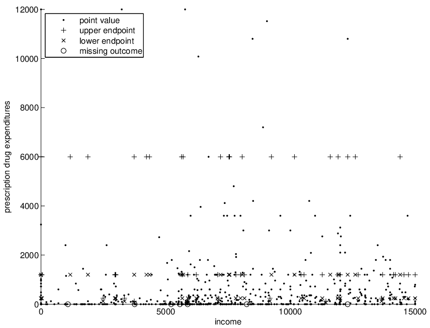


| nominal 90% coverage | |||||
|---|---|---|---|---|---|
| estimated rate | 0.873 | 0.890 | 0.897 | 0.889 | 0.879 |
| conservative rate () | 0.991 | 0.987 | 0.987 | 0.995 | 0.996 |
| (infeasible) exact rate () | 0.921 | 0.909 | 0.905 | 0.903 | 0.890 |
| nominal 95% coverage | |||||
| estimated rate | 0.940 | 0.943 | 0.954 | 0.947 | 0.934 |
| conservative rate () | 0.998 | 1.000 | 0.998 | 1.000 | 0.999 |
| (infeasible) exact rate () | 0.976 | 0.965 | 0.949 | 0.956 | 0.953 |
| nominal 90% coverage | |||||
|---|---|---|---|---|---|
| estimated rate | 0.780 | 0.910 | 0.928 | 0.925 | 0.924 |
| conservative rate () | 0.949 | 0.947 | 0.938 | 0.932 | 0.924 |
| (infeasible) exact rate () | 0.949 | 0.947 | 0.938 | 0.932 | 0.924 |
| nominal 95% coverage | |||||
| estimated rate | 0.885 | 0.945 | 0.966 | 0.971 | 0.979 |
| conservative rate () | 0.991 | 0.982 | 0.975 | 0.974 | 0.979 |
| (infeasible) exact rate () | 0.991 | 0.982 | 0.975 | 0.974 | 0.979 |
| nominal 90% coverage | |||||
|---|---|---|---|---|---|
| estimated rate | 0.26 | 0.13 | 0.08 | 0.06 | 0.03 |
| conservative rate () | 0.33 | 0.17 | 0.12 | 0.09 | 0.06 |
| (infeasible) exact rate () | 0.21 | 0.10 | 0.07 | 0.05 | 0.03 |
| nominal 95% coverage | |||||
| estimated rate | 0.35 | 0.17 | 0.11 | 0.07 | 0.05 |
| conservative rate () | 0.39 | 0.22 | 0.15 | 0.11 | 0.07 |
| (infeasible) exact rate () | 0.29 | 0.13 | 0.09 | 0.06 | 0.04 |
| nominal 90% coverage | |||||
|---|---|---|---|---|---|
| estimated rate | 0.11 | 0.08 | 0.06 | 0.04 | 0.02 |
| conservative rate () | 0.20 | 0.09 | 0.06 | 0.04 | 0.02 |
| (infeasible) exact rate () | 0.20 | 0.09 | 0.06 | 0.04 | 0.02 |
| nominal 95% coverage | |||||
| estimated rate | 0.18 | 0.10 | 0.07 | 0.05 | 0.03 |
| conservative rate () | 0.27 | 0.11 | 0.08 | 0.05 | 0.03 |
| (infeasible) exact rate () | 0.27 | 0.11 | 0.08 | 0.05 | 0.03 |
| Estimated Rate | ||
|---|---|---|
| Conservative Rate | ||
| LAD with Points |