Constraining Thawing Dark Energy using Galaxy Cluster Number Counts
Abstract
We study the formation of galaxy clusters in the presence of thawing class of scalar field dark energy. We consider cases where the scalar field has canonical as well non canonical kinetic term in its action. We also consider various form for the potential of the scalar field e.g, linear, quadratic, inverse quadratic, exponential as well as Pseudo-Nambu-Goldstone Boson (PNGB) type. Moreover we investigate situation where dark energy is homogeneous as well as the situation where dark energy takes part in virialization process. We use the Sheth-Tormen formalism while calculating the number density of galaxy clusters. Our results show that cluster number density for different dark energy models have significant deviation from the corresponding value for the CDM case. The deviation is more for higher redshifts. Moreover the tachyon type scalar field with linear potential has the highest deviation from the CDM case. For the total cluster number counts, different dark energy models can have substantial deviation from CDM and this deviation is most significant around for all the models we considered. We also constrain thawing class of models using the presently available data for number counts of massive X-ray clusters. The results show that current cluster data is not suitable enough for constraining potentials for the thawing scalar fields as well as for other cosmological parameters like . But one can get significant constraint for the parameter and a lower bound on .
Keywords:
Cosmology: Dark Energy, Thawing Model, Halos mass Function, Sheth-Tormen formalism.1 Introduction
Over the last decade, the observational data from Supernovae Type Ia (SNIa) (Kowalski et al., 2008; Riess et al., 2009), Cosmic Microwave Background Radiation (CMBR)(Komatsu et al., 2011), Baryon Acoustic Oscillations (BAO)(Percival et al., 2009) and the large scale structure surveys (Cole et al., 2005) have confirmed that our Universe at present is going through an accelerated expanding phase. Till date, there has been a large number of proposals to explain such an accelerated expansion. This includes the inclusion of an unknown homogeneous matter component having a large negative pressure (cosmological constant being the simplest example of such fluid), modification of gravity at large scale as well as considering the back-reaction of small scale inhomogeneities in the matter distribution.
Although inclusion of cosmological constant in the energy budget of the universe is a minimal way to explain the late time cosmological acceleration which is also allowed by all cosmological observations, but at the same time it is plagued with the fine tuning and the cosmic coincidence problems (Weinberg, 1986; Sahni & Starobinsky, 2000; Carroll, 2001). Scalar field models with generic features can alleviate these problems and provide an alternative to cosmological constant. These dynamical scalar field models of dark energy are broadly classified into two categories: fast roll and slow roll models dubbed freezing and thawing models. For details, see the reference (Caldwell & Linder, 2005). Among these, thawing scalar field models are particularly interesting as they can naturally mimic equation of state very close to which is preferred by all the observational data.
On the other hand, information about the abundance of collapsed structures as a function of mass and redshift is an important tool to study the matter distribution in the universe (Evrard et al., 2002). A large number of cluster surveys are ongoing or being planned to be set-up in near future, e.g., PLANCK, eROSITA, WFXT which would detect a large number of clusters (Vikhlinin et al., 2009b). Indeed, the mass functions of galaxy clusters have been measured through X-ray surveys (Borgani et al., 2001; Reiprich & Bohringer, 2002; Vikhlinin et al., 2009a), via weak and strong lensing studies (Bartelmann et al., 1998; Dahle, 2006; Corless & King, 2009), using optical surveys, like the SDSS (Bahcall et al., 2003; Wen, 2010) as well as through Sunayev-Zeldovich effect (Tauber, 2005). In the last decade several authors have been involved in such studies and have found that the dark energy not only affects the expansion rate of the background and the distance-redshift relation but also the growth of structure in the Universe (Weinberg & Kamionkowski, 2003; Wang & Steinhardt, 1998; Manera & Mota, 2006; Liberato & Rosenfeld, 2006; Nunes & Mota, 2006; Francis et al., 2009; Mortonson, 2009; Pace et al., 2010; Khedekar et al., 2010b; Khedekar & Majumdar, 2010b; Basilakos et al., 2009; Basilakos et al., 2010). The investigation by Basilakos et al. (2010) is particularly interesting in this regard. They have analyzed the predicted cluster-size halo redshift distribution on the bass of two cluster surveys: one is the future X-ray survey based on the e-Rosita satellite and the other one is the Sunayev-Zeldovich survey based on the South Pole Telescope. They found that the predictions of most of the popular dark energy models can be clearly distinguished from the concordance CDM model based on the observations that one can have from these two surveys. Hence dark energy is expected to have an impact on observables such as cluster number counts and lensing statistics (Evrard et al., 2002). Therefore, the studies of galaxy clusters would provide a useful tool to constrain the model parameters and would help to infer the properties of dark energy by discriminating among the different dark energy models.
Although the proper way to understand the effect of dark energy in the non-linear regime of structure formation is through the N-body numerical simulations (Baldi et al., 2010; Courtin et al., 2011; Macci et al., 2004), one can also use a simpler semi-analytical methods which are in reasonable agreement with N-body simulations. One such example is the spherical collapse model (Gunn & Gott, 1972) using the Press-Schechter formalism(Press & Schechter, 1974). To overcome the problem of over-prediction of number of low(high) mass halos at the current epoch for the above model, an elliptical collapse model was later proposed by Sheth & Tormen (1999).
This paper extends the previous work by Devi & Sen (2011) by further studying the most general analytic form of halo mass function introduced by Sheth & Tormen (1999) for thawing type scalar field dark energy models with various potential and examine how does the DE affect the abundance of CDM halos by measuring the galaxy cluster number counts. We consider both the canonical and non-canonical form of thawing dark energy models. For the completeness of the study we check the results for homogeneous as well as inhomogeneous dark energy cases. We discuss how much they deviate from the conventional CDM model through the linearly extrapolated density contrast at the redshift of collapse, the number density of halo mass at some particular redshifts of collapse and also through the total cluster number counts.
In a recent paper Campanelli et al. (2011) have studied the constraints on different dark energy models through cluster number counts. They assumed the CPL parametrization (Linder, 2003; Chevallier & Polarski, 2001) to model different dark energy models. But it was recently shown by Gupta, Majumdar & Sen (2012) that this parametrization does not correctly represent all the thawing class of scalar field models. Moreover this parametrization is also not suitable for thawing scalar fields with non canonical kinetic term. Hence in our analysis, we do not assume any parametrization that represents thawing class of models. Instead, we consider the full system of coupled scalar field plus Einstein’s equations for the thawing class of scalar fields.
We also put constraints on our model using the presently available cluster number data from massive X-ray clusters as obtained by Campanelli et al. (2011). In doing this we concentrate on canonical scalar field models that deviate significantly from CDM behaviour. The results shows that present data is not suitable to constrain the thawing scalar field potentials as well as other cosmological parameters like , although one can get significant constrain on the parameter , the rms mass fluctuation today at scale and a lower bound on .
The structure of the paper is as follows: in section 2, we introduce the thawing dark energy models for both canonical and non-canonical kinetic term. We discuss the background evolution for such fields considering the difference type of potentials e.i. , , and and also PNGB type. In section 3, we sketch the derivation of the equations to calculate the linearly extrapolated density contrast, , at the collapsed redshift. Then, we describe the halos mass function introduced by Sheth & Tormen (1999) and calculate the number density and the total cluster number counts for our DE models. In section 4, we discuss the observational constrain on the thawing models and finally we draw conclusions in section 5.
2 Background Evolution
In what follows, we consider a flat, homogeneous and isotropic background universe driven by non-relativistic matter and dark energy of thawing type, i.e. . These thawing type dark energy models are characterized by the fact that in the early universe the scalar field is frozen by very large Hubble damping and the scalar field starts evolving slowly down its potential at the later time. So, the equation of state, initially starts with and slowly departs from it in the later time. We consider both ordinary scalar field with canonical kinetic term as well as tachyon type scalar field having Born-Infeld type kinetic term which are minimally coupled to the gravity sector (Sen, 2002a; Sen, 2002b; Garousi, 2000; Kluson, 2000). The equation of motions for the canonical scalar field and the tachyon field are given by
| (1) | |||
| (2) |
respectively, where dot represents the differentiation w. r. t the cosmic time and the Hubble parameter, is defined as
| (3) |
Here is the scale factor, is the background matter density and represents the dark energy density with
| (4) |
Defining new variables and for the canonical scalar field model, one can form an autonomous system of equations involving two observable parameters and together with the parameter . For the canonical scalar field, it is given as
| (5) | |||||
| (6) | |||||
| (7) |
For detail derivations of the above equations, see Scherrer & Sen (2008a). Here the prime denotes derivative with respect to ln. We solve this system of equations numerically for the mentioned potentials providing the initial conditions for and as , . As discussed in Scherrer & Sen (2008a), one can easily see that smaller the value of , more the scalar field evolution similar to that of cosmological constant . To check for the maximum deviation from the cosmological constant , we set . For we choose its initial value in such away so that to get required value at present. The different types of potential we considered are , , and and they correspond to and respectively. We also considered the Pseudo-Nambu Goldstone Boson model (PNGB) (Frieman et al., 1995) which has been characterized by the potential:
| (8) |
with . To solve the above of system of equations, one needs a third initial condition for . The parameters for the potentials, or can be related to this initial value for . Moreover this initial value for can be related to its value at present, . Hence once we choose the form of the potentials and the initial values for and as mentioned above, the only free parameter for the background evolution is or . The rest of the potential parameters can be known from its value.
Similarly, for the thawing tachyon field models, the autonomous system of equations is given by
| (9) | |||||
| (10) | |||||
| (11) |
where and . Here also we set the initial conditions similar to the canonical scalar field case and consider the power law potentials as mentioned above. For the detail calculations see Scherrer & Sen (2008a); Scherrer & Sen (2008b); Ali et al. (2009). One can see the behaviour of the equation of state parameter from the Figure 1 for the various models we considered. The different models have a maximum deviation when one approaches the present day however they behave almost identically in the past.

3 Halo Mass Function
The studies of the mass function of collapsed objects like clusters of galaxies can be used to constrain the cosmological models and can help to infer the properties of dark energy. In what follows we calculate the halo mass function for the DE models considered in this paper.
3.1 Spherical collapse
As our interests lie in finding the halo-mass of CDM matter in presence of thawing dark energy, we need to study the perturbation of matter inhomogeneity in order to calculate the linear density contrast at the time of collapse. We refer the readers to Mota (2008) and Basilakos et al. (2009) for some earlier works regarding spherical collapse formalism with dark energy models. We consider a spherical region of radius evolving in a cosmologically expanding background. The dynamics of this spherical region is essentially governed by the Raychaudhuri equation,
| (12) |
where and are the density of scalar field and the matter density inside the cluster respectively. It is easier to solve the equations after normalizing at the turn around point, so we define new variables:
| (13) |
where the subscript denotes the turn around time. Now, the equations of background evolution and that of perturbation reduce to
| (14) |
and
| (15) |
where the function is given by (Basilakos & Voglis, 2007)
| (16) |
with
| (17) |
Here represents the matter density contrast at turnaround which is defined as
| (18) |
The function is given by and by
| (19) |
We assume here that the equation of dark energy has the same form inside and outside the cluster. This is purely an assumption to simplify the analysis and is not necessarily true. But one should note that the is function of the background scale factor outside the cluster, but inside the cluster, it is a function of the radius of the spherical region. Hence the actual behavior of the equation of state with time will be different inside and outside the over density, which is similar to the work by Basilakos et al. (2009).

In addition, the linear density contrast obeys the equation:
| (20) |
We calculate the linear over density at the epoch when the spherical region described by equation (12) collapses to a point, by solving equation (20). Here we assume that the virialization epoch is approximately twice of the turn around epoch. We should mention that this condition may get violated in some cases, like a dark energy model with phantom equation of state. But as we are considering here scalar field models, we never go to the phantom region of the equation of state. Hence this relation still holds for our case. For the initial condition , we write
| (21) |
so that,
| (22) |
Here is the constant term which can be found by solving equations (14) and (15) after substituting equations (21) and (22). We neglect the higher order terms in . For our case the initial conditions on are found out as
| (23) |
As we are dealing with second-order equations, two initial values are required, one for the initial over-density and other is the initial rate of evolution, . The quantity is generally set to . However we set since the result does not change considerably. The initial epoch is set to .
3.2 Number counts
With the indication from observations that individual galaxies and cluster of galaxies are embedded in extended halos of dark matter, the abundance of CDM halos have been studied widely. Theoretically, Press and Schetcher were the first to describe the abundance of these CDM halos as a function of their mass with the assumption that the fraction of the volume of the universe that has collapsed into objects of mass at a redshift follows a Gaussian distribution. The comoving number density of clusters which have collapsed (i.e., virialized) at certain redshift and have masses in the range can be expressed as:
| (24) |
where is defined as mass function. The standard Press-shechter mass function is of the form :
| (25) |
Although it provides a good general representation of the observed distribution of clusters, due to the discrepancy of over-prediction (under-prediction) of the number of low (high) mass halos at the current epoch, Sheth & Tormen (1999) introduced an ellipsoidal model of the collapse of perturbations. This Sheth-Tormen (ST) mass function gives better fits to simulated mass function by reducing this discrepancy substantially. It has the form:
| (26) |
it contains three parameters and which we set into and for all the models we considered. The Press-Shechter case is recovered for and .
It is worth mentioning here that the accuracy of the ST mass function has been found to be limited. In fact, recent high-quality N-body simulations have been used to find fitting functions which work far better than ST mass function for varying dark energy models (Basilakos et al., 2010; Bhattacharya et al., 2011). However, we would keep working with the ST mass function in this paper, keeping in mind that this may introduce errors in our calculations (Reed et al., 2007). Since we are only studying the viability of using future surveys in distinguishing between dark energy models, this much error can be tolerated at this stage. In case one wants to study, e.g., precision cosmology with future cluster data, a much more sophisticated fit would be mandatory.

| Model | Potential | Case | |||
|---|---|---|---|---|---|
| inhom | |||||
| hom | |||||
| inhom | |||||
| hom | |||||
| Scalar | inhom | ||||
| hom | |||||
| inhom | |||||
| hom |
The dispersion of the density field on a given comoving scale , containing mass , is given by
| (27) |
where the quantity is the power spectrum of density fluctuations extrapolated to according to linear theory and is the top-hat window function;
| (28) |
represents the growth function of linear perturbation theory and can be found from equation(20) (see fig.4 in Schaefer & Koyama (2004)). We normalize the growth function such that at the present epoch.
Assuming that the baryon density parameter , the CDM power spectrum can be approximated by , where is a normalization constant and we use the transfer function, introduced by Eisenstein and Hu (Eisenstein & Hu, 1998a).
The normalization of the power spectrum is often expressed in terms of , the rms fluctuation today at a scale of 8 Mpc. However, since the differences between various dark energy models is usually most prominent at lower redshifts, normalizing the power spectrum using could lead to erroneous results. We rather normalize using the observed CMBR power spectrum amplitude (Basilakos et al., 2010):
| (29) |
where Mpc-1 is a characteristic length probed by CMBR observations (Komatsu et al., 2009).
The number of clusters in a redshift interval , above a given minimum (threshold) mass is obtained from :
| (30) |
where is the fraction of the sky being observed and the comoving volume element is given by
| (31) |
is the comoving radial distance out to redshift z:
| (32) |
where is the Hubble parameter. For numerical computation, the upper limit of integration in equation (30) is replaced by some finite mass value . The comoving volume element is required since the redshift evolution of a physical volume in space is model dependent, i.e, depending on the form of potentials.
3.3 Comparison of Thawing Models with CDM
In this section, we discuss the results for the linear over-density contrast, the number density of CDM halos and the total clusters number counts for the models we introduced, keeping the CDM model as a reference since the CDM model is currently the simplest model, fitting all available observational data despite of its conceptual problems.
In Fig.2, we show the linear density contrast, , as a function of collapsed redshift for both homogeneous (left panel) and inhomogeneous (right panel) scalar field models with various potentials. Similar behavior is being shown for the case of tachyon field in Fig.3. From Figs.2 and 3, it can be seen that the linear density contrast at has a significant deviation from the CDM case for homogeneous dark energy models. These deviations are comparatively smaller in case of inhomogeneous dark energy. This is true for both ordinary scalar field as well as tachyon type scalar field. This type of behavior is expected. For homogeneous case, the equation of state of dark energy is greater than (we are not considering Phantom models). Hence the repulsive effect of dark energy in the background evolution is lesser than the CDM case. This results larger linear density contrast for homogeneous dark energy. However, for inhomogeneous case, there is an extra repulsive effect inside the cluster due to inhomogeneous dark energy. This reduces the linear density contrast for inhomogeneous DE and brings it closer to the CDM value. At high redshift, all the models asymptotically approach to the Einstein-de Sitter (EDS) limit. Among the potentials we considered, the linear potential shows maximum deviation from the CDM for the ordinary and tachyon fields in both the homogeneous and inhomogeneous cases. This is consistent with the results earlier obtained by Devi & Sen (2011).


In passing, we would like to mention that one can find a fitting formula of the linear density contrast for the different models like Abramo et al. (2007) as a function of and redshift. Following Abramo et al. (2007); Weinberg & Kamionkowski (2003); Shaw & Mota (2008), the fitting formula for the scaler field with canonical kinetic term has the form of
| (33) |
The values of parameters and are different according to the model. Considering the canonical scalar field model, we have listed out the corresponding values in the Table 1. One can also find the similar kind of the fitting formula for other models. We compare the accuracy of this fitting formula plotting with the actual data in Fig 4 and one can easily see that the match is excellent.
Next, we investigate a quantity closely related to observations, the clusters number density, . Since it is only depends on and on the growth factor, no appreciable differences are expected between the models studied. In order to see the significant deviation in the cluster number density for the thawing models from that of the standard CDM, we define a new parameter, such that
| (34) |
This parameter measures the deviation in the clusters number density of any thawing models from that of CDM. Larger the value of more it deviates from CDM. The behavior of for the ordinary scalar field as well as for the tachyon type field have been shown in Figs.(5) and (6) respectively. It can be seen from Fig.(5) that value is lower for higher , i.e., the clusters number density for the object collapsing earlier have significant deviation from that of CDM. This is true for both ordinary scalar field and tachyon field in homogeneous as well as inhomogeneous DE cases. The difference between the homogeneous and inhomogeneous is prominent for the object collapsing at the later time (i.e. at redshift ). Again if we look further, the tachyon field models show larger deviations from the CDM at all redshifts than the scalar field with canonical kinetic term. Among the potentials we considered, the linear potential again shows the maximum deviation for the tachyon dark energy models for homogeneous as well as inhomogeneous cases.
An another important quantity that can be derived from observations is the total number counts of CDM halos above a given mass in a complete survey volume. There are a number of cluster surveys ongoing or being planned in near future, e.g., PLANCK, eROSITA, WFXT which would detect a large number of clusters (Vikhlinin et al., 2009b). To obtain the mass of the clusters detected, one usually utilizes a proxy variable which can be the X-ray flux, SZE flux or richness of the cluster. The actual quantity chosen would, of course, depend on the nature of the survey. The relation between these quantities and the mass depends on the detailed cluster physics. However, for our purpose, it suffices to state that the limiting mass of the survey will be essentially determined by the limits on the proxy variable.
For predicting the number of clusters that would be detected in future surveys, we choose two specific surveys, namely, (i) the eROSITA satellite X-ray survey, which is expected to have a flux limit ergs s-1 cm-2 at the energy band 0.5-5 keV and would cover deg2 of the sky (corresponding to a fraction ), and (ii) the South Pole Telescope SZ survey (SPT), which has a limiting flux density mJy at the frequency GHz and a sky coverage of deg2 (corresponding to a fraction ). The method of converting these limiting fluxes to limiting halo masses for the two surveys is outlined in Fedeli, Moscardini & Matarrese (2009) and Basilakos et al. (2010). We simply follow their prescription and refer the reader to the above papers for details.
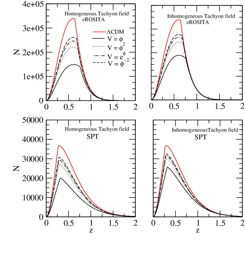
We show the calculated value of the total number counts of haloes as the function of redshift in Figures 7 and 8 for all the models we considered as indicated in the figures. The top panels correspond to our predictions for eROSITA while the bottom panels are for SPT. We discuss the results below.
It is clear that there exists significant difference in the number counts between different DE models considered. The difference is most significant around . To take a specific example, we see from the top-left panel of Figure 7 that the difference in number counts (as would be observed in eROSITA) between CDM and homogeneous scalar field model is at . This difference is significantly larger than the statistical uncertainties (which would be for the survey we are considering), and hence can be used for discriminating between different models. The corresponding difference in the two models for SPT is at (see the bottom-left panel), while the corresponding statistical uncertainties would be . Hence, the two surveys could, in principle, be able to distinguish between CDM and the other DE models. The same conclusions can be drawn from other panels as well, and also for tachyonic fields shown in Figure 8. We should mention that discriminating between different DE models would be limited by our ignorance of other cosmological parameters like . A proper analysis of how to constrain the models would involve error estimates of the parameters. In the next section, we make a brief attempt in this regard.
4 Observational Constraints
4.1 Cluster Data
| bin | Ref. | |||||
|---|---|---|---|---|---|---|
| 1 | 0.00 | 0.10 | 0.050 | Ikebe et al. (2002) | 0.309 | |
| 2 | 0.30 | 0.50 | 0.375 | Henry (2000) | 0.012 | |
| 3 | 0.50 | 0.65 | 0.550 | Bahcall & Fan (1998), | 0.006 | |
| Bahcall & Bode (2003) | ||||||
| 4 | 0.65 | 0.90 | 0.825 | Donahue et al. (1998) | 0.001 |
| bin 1 | bin 2 | bin 3 | bin 4 | ||
|---|---|---|---|---|---|
| [ | |||||
| [ | |||||
| [ | |||||
| [ | |||||
| [ |
In this section, we use observational data for cluster abundances to constrain the thawing class of models that behave significantly different from CDM model.
In this regard we follow the recent treatment by Campanelli et al. (2011) to calculate the observed galaxy number counts from the X-Ray temperature measurements for massive clusters and the subsequent statistical analysis.
The comoving number for the clusters within the redshift range between and , with mass greater than is given by Campanelli et al. (2011):
| (35) |
where is the comoving cluster number density at redshift for those clusters which have masses greater than and is given by equation (30). Following Bahcall & Fan (1998) and Bahcall & Bode (2003), we assume with corresponding comoving radius . We assume for the solar mass. As mention earlier represents the effective fraction of the total comoving volume that is observed at redshift .
Subsequently, we show in Table 2, four redshift bins centered at some redshift . This has been taken from the analysis by Campanelli et al. (2011) (See also the corresponding references). In the table, the value of the effective fraction of the total comoving volume are also listed which have been computed using the results of (Bahcall & Fan, 1998; Bahcall & Bode, 2003). Usually the parameter depends on the underlying cosmology but this dependence is weak as observed in Campanelli et al. (2011). Subsequently for i-th bin, we write
| (36) |
where is the effective fraction in the bin listed in Table 2.
Next one uses the X-ray temperature measurements for massive clusters and then convert the temperature measurements to the mass measurements. The detail of this procedure is given in the recent analysis by Campanelli et al. (2011). We skip this detailing and quote the corresponding data for observed number of clusters in Table 3 as obtained by Campanelli et al. (2011).
The quantity in Table 3 is defined as:
| (37) |
The quantity is the virial over-density which depends on redshift and cosmology. For our case it has been thoroughly discussed in Devi & Sen (2011) and in Appendix C of Campanelli et al. (2011).
4.2 Data Analysis and Results
Due to a small data set, one can do the data analysis assuming the error distribution to follow a Poisson statistics. Following Campanelli et al. (2011), we write the in our case as:
| (38) | |||
Following Campanelli et al. (2011) we also take into account the uncertainty in the comoving numbers of clusters, , by introducing another parameter to modify the as
| (39) | |||
where .
As we are interested in thawing models which differ substantially from CDM behaviour, we fix . We also fix for our subsequent analysis. In this present analysis, we consider the thawing models with canonical scalar fields and consider only the inhomogeneous scalar field case.


We marginalise over the parameter with uniform prior. With this, the is a function of four parameters, e.g and . The last one is a parameter related to the scalar field thawing model. It determines the form of the potential. For i.e for the linear potential, we show the confidence contours in the plane in figure 9. This shows that there is no bound on . In other words, the cluster data that we have used, can not constrain . This is also true for other potentials. Hence in our subsequent analysis we fix which is the best fit value obtained by WMAP-7, Komatsu et al. (2011).
We are now left with three parameters: two cosmological parameters, and and one model parameter . The results are shown in figures 10 and 11. From figure10, it is clear that we get a bound in the plane which is similar to bounds obtained in other works Campanelli et al. (2011). On the other hand, figure 11 implies that although one can get a strong constraint on the parameter , it is not possible to constrain the form of the potential for the thawing models as the parameter is unconstrained. This is hardly surprising as we have already seen that the data on cluster counts can distinguish between thawing models mainly in the redshift range . However, the data set used in this analysis contains only three clusters in this redshift range. Using the parameters appropriate for these observations, we find that the difference in the cluster counts for various models is of the order of a few, which is similar to the statistical uncertainties. In other words, we can not constrain the thawing dark energy potentials with such a small number of clusters at . As we have mentioned earlier, large cluster surveys with substantially more number counts () will be useful in constraining the models.
5 Conclusion
To summarize, we investigate the cluster abundance in cosmological scenario where the universe is dominated by the thawing class of scalar dark energy. We consider both the ordinary scalar field with canonical kinetic term as well as tachyon field with DBI form of kinetic energy. Moreover, we consider a variety of potentials that can give rise to suitable cosmological scenario different from concordance CDM model. To study the formation of collapsed structures, we consider homogeneous dark energy as well as dark energy scenario where dark energy takes part in the virialisation process. We consider the Press-Schetcher formalism modified by Sheth & Tormen (1999) to calculate the mass function. Subsequently, we show that there exists significant difference in the number counts between different dark energy models and the concordance CDM model. We also constrain our model using presently available observational data for cluster number counts. We show that although the present data is not suitable enough to distinguish thawing class of models, one can still get a reasonably strong constraint on the cosmological parameter as well as a lower bound on the parameter .
Given the fact that a large number of cluster surveys are currently ongoing as well as a number of future surveys are being planned, cluster number counts can be a smoking gun to distinguish different dark energy models from the CDM. Our present work is one preliminary step towards that direction. This work can be extended to freezing class of scalar field models as well as for models with non minimally coupled scalar fields. This will be our future aim.
6 Acknowledgement
AAS acknowledges the financial support provided by the SERC, DST, Govt. of India through the research grant (DST-SR/S2/HEP-043/2009. NCD acknowledges the financial support provided by CSIR, Govt. of India. NCD also acknowledges the Harish-Chandra Research Institute, Allahabad, India for hospitality provided during her visit where part of the work has been done. We thank the anonymous referee for his/her comments which helped us in improving the paper.
References
- Abramo et al. (2007) Abramo L. R., Batista R. C., Liberato L. & Rosenfeld R., 2007, JCAP, 0711, 012
- Ali et al. (2009) Ali A., Sami M., & Sen A. A., 2009, Phys. Rev. D, 79, 123501
- Bahcall et al. (2003) Bahcall N. A., et al., 2003, ApJ., 585, 182
- Bahcall & Fan (1998) Bahcall N. A. & Fan X. 1998, ApJ., 504, 1
- Bahcall & Bode (2003) Bahcall N. A. & Bode P. 2003, ApJ, 588, L1
- Baldi et al. (2010) Baldi M., Pettorino V., Robbers G. & Springel V., 2010, MNRAS, 403, 1684
- Bartelmann et al. (1998) Bartelmann M., Huss A., Colberg J. M., Jenkins A. & Pearce F. R., 1998, Astron. Astrophys., 330, 1
- Basilakos et al. (2010) Basilakos S., Plionis M. & Lima J. A. S., 2010, Phys. Rev. D, 82, 083517
- Basilakos et al. (2009) Basilakos S., Sanchez J. C. B. & Perivolaropoulos L., 2009, Phys. Rev. D, 80, 043530
- Basilakos & Voglis (2007) Basilakos S. & Voglis N., 2007, MNRAS, 374, 269,
- Bhattacharya et al. (2011) Bhattacharya S., Heitmann K., White M., et al., 2011, ApJ., 732, 122
- Borgani et al. (2001) Borgani S., et al., 2001, ApJ., 561, 13
- Caldwell & Linder (2005) Caldwell R. R. & Linder E. V., 2005, Phys. Rev. Lett., 95, 141301
- Campanelli et al. (2011) Campanelli L., Fogli G. L., Kahniashvili T., Marrone A. & Bharat Ratra, 2011, [arXiv:1110.2310]
- Carroll (2001) Carroll S. M., 2001, Living Rev. Rel., 4, 1
- Chevallier & Polarski (2001) Chevallier M. & Polarski D., 2011 Int. J. Mod. Phys. D, 10, 213
- Cole et al. (2005) Cole S., et al., 2005, MNRAS, 362, 505
- Corless & King (2009) Corless V. L. & King L. J., 2009, MNRAS, 396, 315
- Courtin et al. (2011) Courtin J. et al., 2011, MNRAS, 410, 1911
- Dahle (2006) Dahle H., 2006, ApJ, 653, 954
- Devi & Sen (2011) Devi N. C. & Sen A. A., 2011, MNRAS, 413, 2371
- Donahue et al. (1998) Donahue M. et al., 1998, ApJ, 502, 550
- Eisenstein & Hu (1998a) Eisenstein D. J. & Hu W., 1998a, ApJ, 496, 605
- Evrard et al. (2002) Evrard A. E., et al., 2002, ApJ., 573, 7
- Fedeli, Moscardini & Matarrese (2009) Fedeli C., Moscardini L. & Matarrese S., 2009, MNRAS, 397, 1125
- Francis et al. (2009) Francis M. J., Lewis G. F. & Linder G. F., 2009, MNRAS, 393, L31
- Frieman et al. (1995) Frieman J. A., Hill C. T., Stebbins A. & Waga I., 1995, Phys. Rev. Lett., 75, 2077
- Garousi (2000) Garousi M. R., 2000, Nuclear Phys. B, 584, 284
- Gunn & Gott (1972) Gunn J. E. & Gott J. R., 1972, ApJ, 176, 1
- Gupta, Majumdar & Sen (2012) Gupta G., Majumdar S. & Sen, A. A., 2012, MNRAS, 420, 1309
- Henry (2000) Henry J. P. 2000, ApJ, 534, 565
- Ikebe et al. (2002) Ikebe Y. Reiprich T. H. Boehringer H. Tanaka Y. & Kitayama T. 2002, Astron. Astrophys. 383, 773
- Kluson (2000) Kluson J., 2000, Phys. Rev. D, 62, 126003
- Khedekar et al. (2010b) Khedekar S., Das S. & Majumdar S., 2010a, Phys. Rev. D, 82, 1301
- Khedekar & Majumdar (2010b) Khedekar S. & Majumdar S., 2010b, Phys. Rev. D, 82, 081301
- Komatsu et al. (2009) Komatsu E., et al., 2009, Astrophys. J. Suppl. 180, 330
- Komatsu et al. (2011) Komatsu E., et al., 2011, Astrophys. J. Suppl. 192, 18
- Kowalski et al. (2008) Kowalski M., et al., 2008, ApJ, 686, 749
- Liberato & Rosenfeld (2006) Liberato L. & Rosenfeld R., 2006, JCAP, 7, 9
- Linder (2003) Linder E. V., 2003, Phys. Rev. Lett. 90, 091301
- Macci et al. (2004) Maccio A. V., Quercellini C., Mainini R., Amendola L. & Bonometto S. A., 2004, Phys. Rev. D, 69, 123516
- Manera & Mota (2006) Manera M. & Mota D. F., 2006, MNRAS, 371, 1373
- Mota (2008) Mota D. F. 2008, JCAP, 9, 6
- Mortonson (2009) Mortonson M. J., 2009, Phys. Rev. D, 80, 123504
- Nunes & Mota (2006) Nunes N. J. & Mota D. F., 2006, MNRAS, 368, 751
- Pace et al. (2010) Pace F., Waizmannm J-C. & Bartelman M., 2010, MNRAS, 406, 1865
- Percival et al. (2009) Percival W. J., et al., 2009, MNRAS, 401, 2331.
- Press & Schechter (1974) Press W. H. & Schechter P., 1974, ApJ, 187, 425
- Reed et al. (2007) Reed D. S., Bower R., Frenk C. S., Jenkins A. & Theuns T., 2007, MNRAS, 374, 2
- Reiprich & Bohringer (2002) Reiprich T. H. & B¨ohringer H., 2002 ApJ., 567, 716,
- Riess et al. (2009) Riess A. G., et al., 2009, ApJ, 699, 539
- Sahni & Starobinsky (2000) Sahni V. & Starobinsky A., 2000, Int. J. Mod. Phys. D, 9, 373
- Schaefer & Koyama (2004) Schaefer B. M. & Koyama K., 2008, MNRAS, 385, 411
- Scherrer & Sen (2008a) Scherrer R. J. & Sen A. A., 2008a Phys. Rev. D, 77, 083515
- Scherrer & Sen (2008b) Scherrer R. J. & Sen A. A., 2008b Phys. Rev. D, 78, 067303
- Sen (2002a) Sen A., 2002a, J. High Energy Phys., 0204, 048
- Sen (2002b) Sen A., 2002b, Mod. Phys. Lett. A, 17, 1797
- Shaw & Mota (2008) Shaw D. J. & Mota D. F., 2008, ApJS, 174, 277
- Sheth & Tormen (1999) Sheth R. K. & Tormen G., 1999, MNRAS, 308, 119
- Tauber (2005) Tauber J. A., 2005, New Cosmological Data and the values of the Fundamental Parameters, 201, 86
- Vikhlinin et al. (2009a) Vikhlinin A., et al., 2009, ApJ., 692, 1060
- Vikhlinin et al. (2009b) Vikhlinin A., et al., 2009b, [arXiv:0903.5320]
- Wang & Steinhardt (1998) Wang L. & Steinhardt P. J., 1998, ApJ, 508, 483
- Weinberg (1986) Weinberg S., 1986, Rev. Mod. Phys., 61, 1
- Weinberg & Kamionkowski (2003) Weinberg N. N. & Kamionkowski M., 2003, ApJ, 341, 251
- Wen (2010) Wen Z. L., Han J. L. & Liu F. S., 2010, 2010, MNRAS, 407, 533