跳到论文正文
W Papers独立论文阅读器 arXiv:1112.0708 论文正文 计算阅读时间 · 0%
引用这篇论文根据当前论文元数据生成,正式投稿前建议核对。


License: arXiv.org perpetual non-exclusive license
arXiv:1112.0708v2 [cs.IT] 19 Jan 2013

Information-Theoretically Optimal Compressed Sensing via
Spatial Coupling and Approximate Message Passing

David L. Donoho†    Adel Javanmard*    Andrea Montanari Note: Department of Electrical Engineering, Stanford University Note: Department of Statistics, Stanford University
This work was presented in part at the 2012 IEEE International Symposium on Information Theory
Abstract

We study the compressed sensing reconstruction problem for a broad class of random, band-diagonal sensing matrices. This construction is inspired by the idea of spatial coupling in coding theory. As demonstrated heuristically and numerically by Krzakala et al. [KMS+11], message passing algorithms can effectively solve the reconstruction problem for spatially coupled measurements with undersampling rates close to the fraction of non-zero coordinates.

We use an approximate message passing (AMP) algorithm and analyze it through the state evolution method. We give a rigorous proof that this approach is successful as soon as the undersampling rate δ\delta exceeds the (upper) Rényi information dimension of the signal, d¯​(pX)\overline{d}(p_{X}). More precisely, for a sequence of signals of diverging dimension nn whose empirical distribution converges to pXp_{X}, reconstruction is with high probability successful from d¯​(pX)​n+o​(n)\overline{d}(p_{X})\,n+o(n) measurements taken according to a band diagonal matrix.

For sparse signals, i.e., sequences of dimension nn and k⁡(n)k(n) non-zero entries, this implies reconstruction from k⁡(n)+o⁡(n)k(n)+o(n) measurements. For ‘discrete’ signals, i.e., signals whose coordinates take a fixed finite set of values, this implies reconstruction from o⁡(n)o(n) measurements. The result is robust with respect to noise, does not apply uniquely to random signals, but requires the knowledge of the empirical distribution of the signal pXp_{X}.

1 Introduction and main results

1.1 Background and contributions

Assume that mm linear measurements are taken of an unknown nn-dimensional signal x∈ℝnx\in{\mathbb{R}}^{n}, according to the model

y=A​x.\displaystyle y=Ax\,. (1)

The reconstruction problem requires to reconstruct xx from the measured vector y∈ℝmy\in{\mathbb{R}}^{m}, and the measurement matrix A∈ℝm×nA\in{\mathbb{R}}^{m\times n}.

It is an elementary fact of linear algebra that the reconstruction problem will not have a unique solution unless m≥nm\geq n. This observation is however challenged within compressed sensing. A large corpus of research shows that, under the assumption that xx is sparse, a dramatically smaller number of measurements is sufficient [Don06a, CRT06a, Don06b]. Namely, if only kk entries of xx are non-vanishing, then roughly m≳2​k​log⁡(n/k)m\gtrsim 2k\log(n/k) measurements are sufficient for AA random, and reconstruction can be solved efficiently by convex programming. Deterministic sensing matrices achieve similar performances, provided they satisfy a suitable restricted isometry condition [CT05]. On top of this, reconstruction is robust with respect to the addition of noise [CRT06b, DMM11], i.e., under the model

y=A​x+w,\displaystyle y=Ax+w\,, (2)

with, say, w∈ℝmw\in{\mathbb{R}}^{m} a random vector with i.i.d. components wi∼𝖭⁡(0,σ2)w_{i}\sim{\sf N}(0,\sigma^{2}) (unless stated otherwise, σ=0\sigma=0 is a valid choice). In this context, the notions of ‘robustness’ or ‘stability’ refers to the existence of universal constants CC such that the per-coordinate mean square error in reconstructing xx from noisy observation yy is upper bounded by C​σ2C\,\sigma^{2}.

From an information-theoretic point of view it remains however unclear why we cannot achieve the same goal with far fewer than 2​k​log⁡(n/k)2\,k\log(n/k) measurements. Indeed, we can interpret Eq. (1) as describing an analog data compression process, with yy a compressed version of xx. From this point of view, we can encode all the information about xx in a single real number y∈ℝy\in{\mathbb{R}} (i.e., use m=1m=1), because the cardinality of ℝ{\mathbb{R}} is the same as the one of ℝn{\mathbb{R}}^{n}. Motivated by this puzzling remark, Wu and Verdú [WV10] introduced a Shannon-theoretic analogue of compressed sensing, whereby the vector xx has i.i.d. components xi∼pXx_{i}\sim p_{X}. Crucially, the distribution pXp_{X} is available to, and may be used by the reconstruction algorithm. Under the mild assumptions that sensing is linear (as per Eq. (1)), and that the reconstruction mapping is Lipschitz continuous, they proved that compression is asymptotically lossless if and only if

m≥n​d¯​(pX)+o⁡(n).\displaystyle m\geq n\,\overline{d}(p_{X})+o(n)\,. (3)

Here d¯​(pX)\overline{d}(p_{X}) is the (upper) Rényi information dimension of the distribution pXp_{X}. We refer to Section 1.2 for a precise definition of this quantity. Suffices to say that, if pXp_{X} is ε{\varepsilon}-sparse (i.e., if it puts mass at most ε{\varepsilon} on nonzeros) then d¯​(pX)≤ε\overline{d}(p_{X})\leq{\varepsilon}. Also, if pXp_{X} is the convex combination of a discrete part (sum of Dirac’s delta) and an absolutely continuous part (with a density), then d¯​(pX)\overline{d}(p_{X}) is equal to the weight of the absolutely continuous part.

This result is quite striking. For instance, it implies that, for random kk-sparse vectors, m≥k+o⁡(n)m\geq k+o(n) measurements are sufficient. Also, if the entries of xx are random and take values in, say, {−10,−9,…,−9,+10}\{-10,-9,\dots,-9,+10\}, then a sublinear number of measurements m=o⁡(n)m=o(n), is sufficient! At the same time, the result of Wu and Verdú presents two important limitations. First, it does not provide robustness guarantees11 1 While this paper was about to be posted, we became aware of a paper by Wu and Verdú [WV11b] proving a robustness guarantee for δ>D¯​(pX)\delta>\overline{D}(p_{X}) for the case of probability distributions that do not contain singular continuous component. The reconstruction method is again not practical. of the type described above. Second and most importantly, it does not provide any computationally practical algorithm for reconstructing xx from measurements yy.

In an independent line of work, Krzakala et al. [KMS+11] developed an approach that leverages on the idea of spatial coupling. This idea was introduced for the compressed sensing literature by Kudekar and Pfister [KP10] (see [KRU11] and Section 1.5 for a discussion of earlier work on this topic). Spatially coupled matrices are, roughly speaking, random sensing matrices with a band-diagonal structure. The analogy is, this time, with channel coding.22 2 Unlike [KMS+11], we follow here the terminology developed within coding theory. In this context, spatial coupling, in conjunction with message-passing decoding, allows to achieve Shannon capacity on memoryless communication channels. It is therefore natural to ask whether an approach based on spatial coupling can enable to sense random vectors xx at an undersampling rate m/nm/n close to the Rényi information dimension of the coordinates of xx, d¯​(pX)\overline{d}(p_{X}). Indeed, the authors of [KMS+11] evaluate such a scheme numerically on a few classes of random vectors and demonstrate that it indeed achieves rates close to the fraction of non-zero entries. They also support this claim by insightful statistical physics arguments.

In this paper, we fill the gap between the above works, and present the following contributions:

Construction.

We describe a construction for spatially coupled sensing matrices AA that is somewhat broader than the one of [KMS+11] and give precise prescriptions for the asymptotic values of various parameters. We also use a somewhat different reconstruction algorithm from the one in [KMS+11], by building on the approximate message passing (AMP) approach of [DMM09, DMM10]. AMP algorithms have the advantage of smaller memory complexity with respect to standard message passing, and of smaller computational complexity whenever fast multiplication procedures are available for AA.

Rigorous proof of convergence.

Our main contribution is a rigorous proof that the above approach indeed achieves the information-theoretic limits set out by Wu and Verdú [WV10]. Indeed, we prove that, for sequences of spatially coupled sensing matrices {A⁡(n)}n∈ℕ\{A(n)\}_{n\in{\mathbb{N}}}, A⁡(n)∈ℝm⁡(n)×nA(n)\in{\mathbb{R}}^{m(n)\times n} with asymptotic undersampling rate δ=limn→∞m⁡(n)/n\delta=\lim_{n\to\infty}m(n)/n, AMP reconstruction is with high probability successful in recovering the signal xx, provided δ>d¯​(pX)\delta>\overline{d}(p_{X}).

Robustness to noise.

We prove that the present approach is robust33 3 This robustness bound holds for all δ>D¯​(pX)\delta>\overline{D}(p_{X}), where D¯​(pX)\overline{D}(p_{X}) is the upper MMSE dimension of pXp_{X}. (see Definition 1.4). It is worth noting that D¯​(pX)=d¯​(pX)\overline{D}(p_{X})=\overline{d}(p_{X}) for a broad class of distributions pXp_{X} including distributions without singular continuous component. to noise in the following sense. For any signal distribution pXp_{X} and undersampling rate δ\delta, there exists a constant CC such that the output x^​(y){\widehat{x}}(y) of the reconstruction algorithm achieves a mean square error per coordinate n−1​𝔼​{‖x^​(y)−x‖22}≤C​σ2n^{-1}{\mathbb{E}}\{\|{\widehat{x}}(y)-x\|_{2}^{2}\}\leq C\,\sigma^{2}. This result holds under the noisy measurement model (2) for a broad class of noise models for ww, including i.i.d. noise coordinates wiw_{i} with 𝔼⁡{wi2}=σ2<∞{\mathbb{E}}\{w_{i}^{2}\}=\sigma^{2}<\infty.

Non-random signals.

Our proof does not apply uniquely to random signals xx with i.i.d. components, but indeed to more general sequences of signals {x⁡(n)}n∈ℕ\{x(n)\}_{n\in{\mathbb{N}}}, x⁡(n)∈ℝnx(n)\in{\mathbb{R}}^{n} indexed by their dimension nn. The conditions required are: (1)(1) that the empirical distribution of the coordinates of x⁡(n)x(n) converges (weakly) to pXp_{X}; and (2)(2) that ‖x⁡(n)‖22\|x(n)\|^{2}_{2} converges to the second moment of the asymptotic law pXp_{X}.

There is a fundamental reason why this more general framework turns out to be equivalent to the random signal model. This can be traced back to the fact that, within our construction, the columns of the matrix AA are probabilistically exchangeable. Hence any vector x⁡(n)x(n) is equivalent to the one whose coordinates have been randomly permuted. The latter is in turn very close to the i.i.d. model. By the same token, the rows of AA are exchangeable and hence the noise vector ww does not need to be random either.

Interestingly, the present framework changes the notion of ‘structure’ that is relevant for reconstructing the signal xx. Indeed, the focus is shifted from the sparsity of xx to the information dimension d¯​(pX)\overline{d}(p_{X}). In other words, the signal structure that facilitates recovery from a small number of linear measurements is the low-dimensional structure in an information theoretic sense, quantified by the information dimension of the signal.

In the rest of this section we state formally our results, and discuss their implications and limitations, as well as relations with earlier work. Section 2.3 provides a precise description of the matrix construction and reconstruction algorithm. Section 4 reduces the proof of our main results to two key lemmas. One of these lemmas is a (quite straightforward) generalization of the state evolution technique of [DMM09, BM11]. The second lemma characterizes the behavior of the state evolution recursion, and is proved in Section 7. The proof of a number of intermediate technical steps is deferred to the appendices.

1.2 Formal statement of the results

We consider the noisy model (2). An instance of the problem is therefore completely specified by the triple (x,w,A)(x,w,A). We will be interested in the asymptotic properties of sequence of instances indexed by the problem dimensions 𝒮={(x⁡(n),w⁡(n),A⁡(n))}n∈ℕ{\cal S}=\{(x(n),w(n),A(n))\}_{n\in{\mathbb{N}}}. We recall a definition from [BM12]. (More precisely, [BM12] introduces the B=1B=1 case of this definition.)

Definition 1.1.

The sequence of instances 𝒮={x⁡(n),w⁡(n),A⁡(n)}n∈ℕ{\cal S}=\{x(n),w(n),A(n)\}_{n\in{\mathbb{N}}} indexed by nn is said to be a BB-converging sequence if x⁡(n)∈ℝnx(n)\in{\mathbb{R}}^{n}, w⁡(n)∈ℝmw(n)\in{\mathbb{R}}^{m}, A⁡(n)∈ℝm×nA(n)\in{\mathbb{R}}^{m\times n} with m=m⁡(n)m=m(n) is such that m/n→δ∈(0,∞)m/n\to\delta\in(0,\infty), and in addition the following conditions hold 44 4 If (μk)k∈ℕ(\mu_{k})_{k\in{\mathbb{N}}} is a sequence of measures and μ\mu is another measure, all defined on ℝ{\mathbb{R}}, the weak convergence of μk\mu_{k} to μ\mu along with the convergence of their second moments to the second moment of μ\mu is equivalent to convergence in 22-Wasserstein distance [Vil08]. Therefore, conditions (a)(a)-(b)(b) are equivalent to the following. The empirical distributions of the signal x⁡(n)x(n) and the empirical distributions of noise w⁡(n)w(n) converge in 22-Wasserstein distance. :

  • (a)(a)

    The empirical distribution of the entries of x⁡(n)x(n) converges weakly to a probability measure pXp_{X} on ℝ{\mathbb{R}} with bounded second moment. Further n−1​∑i=1nxi​(n)2→𝔼⁡{X2}n^{-1}\sum_{i=1}^{n}x_{i}(n)^{2}\to{\mathbb{E}}\{X^{2}\}, where the expectation is taken with respect to pXp_{X}.

  • (b)(b)

    The empirical distribution of the entries of w⁡(n)w(n) converges weakly to a probability measure pWp_{W} on ℝ{\mathbb{R}} with bounded second moment. Further m−1​∑i=1mwi​(n)2→𝔼⁡{W2}≡σ2m^{-1}\sum_{i=1}^{m}w_{i}(n)^{2}\to{\mathbb{E}}\{W^{2}\}\equiv\sigma^{2}, where the expectation is taken with respect to pWp_{W}.

  • (c)(c)

    If {ei}1≤i≤n\{e_{i}\}_{1\leq i\leq n}, ei∈ℝne_{i}\in{\mathbb{R}}^{n} denotes the canonical basis, then lim​supn→∞​maxi∈[n]​‖A⁡(n)​ei‖2≤B\underset{n\to\infty}{\rm{lim\,sup}}\max_{i\in[n]}\|A(n)e_{i}\|_{2}\leq B,
    lim​infn→∞​mini∈[n]​‖A⁡(n)​ei‖2≥1/B\underset{n\to\infty}{\rm{lim\,inf}}\min_{i\in[n]}\|A(n)e_{i}\|_{2}\geq 1/B.

We further say that {(x⁡(n),w⁡(n))}n≥0\{(x(n),w(n))\}_{n\geq 0} is a converging sequence of instances, if they satisfy conditions (a)(a) and (b)(b). We say that {A⁡(n)}n≥0\{A(n)\}_{n\geq 0} is a BB-converging sequence of sensing matrices if they satisfy condition (c)(c) above, and we call it a converging sequence if it is BB-converging for some BB. Similarly, we say 𝒮{\cal S} is a converging sequence if it is BB-converging for some BB.

Finally, if the sequence {(x⁡(n),w⁡(n),A⁡(n))}n≥0\{(x(n),w(n),A(n))\}_{n\geq 0} is random, the above conditions are required to hold almost surely.

Notice that standard normalizations of the sensing matrix correspond to ‖A⁡(n)​ei‖22=1\|A(n)e_{i}\|_{2}^{2}=1 (and hence B=1B=1) or to ‖A⁡(n)​ei‖22=m⁡(n)/n\|A(n)e_{i}\|_{2}^{2}=m(n)/n. The former corresponds to normalized columns and the latter corresponds to normalized rows. Since throughout we assume m⁡(n)/n→δ∈(0,∞)m(n)/n\to\delta\in(0,\infty), these conventions only differ by a rescaling of the noise variance. In order to simplify the proofs, we allow ourselves somewhat more freedom by taking BB a fixed constant.

Given a sensing matrix AA, and a vector of measurements yy, a reconstruction algorithm produces an estimate x^​(A,y)∈ℝn{\widehat{x}}(A;y)\in{\mathbb{R}}^{n} of xx. In this paper we assume that the empirical distribution pXp_{X}, and the noise level σ2\sigma^{2} are known to the estimator, and hence the mapping x^:(A,y)↦x^​(A,y){\widehat{x}}:(A,y)\mapsto{\widehat{x}}(A;y) implicitly depends on pXp_{X} and σ2\sigma^{2}. Since however pX,σ2p_{X},\sigma^{2} are fixed throughout, we avoid the cumbersome notation x^​(A,y,pX,σ2){\widehat{x}}(A,y,p_{X},\sigma^{2}).

Given a converging sequence of instances 𝒮={x⁡(n),w⁡(n),A⁡(n)}n∈ℕ{\cal S}=\{x(n),w(n),A(n)\}_{n\in{\mathbb{N}}}, and an estimator x^{\widehat{x}}, we define the asymptotic per-coordinate reconstruction mean square error as

𝖬𝖲𝖤⁡(𝒮,x^)=lim​supn→∞​1n​‖x^​(A⁡(n),y⁡(n))−x⁡(n)‖2.\displaystyle{\sf MSE}({\cal S};{\widehat{x}})=\underset{n\to\infty}{\rm{lim\,sup}}\,\frac{1}{n}\,\big\|{\widehat{x}}\big(A(n);y(n)\big)-x(n)\big\|^{2}\,. (4)

Notice that the quantity on the right hand side depends on the matrix A⁡(n)A(n), which will be random, and on the signal and noise vectors x⁡(n)x(n), w⁡(n)w(n) which can themselves be random. Our results hold almost surely with respect to these random variables. In some applications it is more customary to take the expectation with respect to the noise and signal distribution, i.e., to consider the quantity

𝖬𝖲𝖤¯​(𝒮,𝗑^)=lim​sup𝗇→∞​1n​𝔼​‖x^​(A⁡(n),y⁡(n))−x⁡(n)‖2.\displaystyle\overline{\sf MSE}({\cal S};{\widehat{x}})=\underset{n\to\infty}{\rm{lim\,sup}}\,\frac{1}{n}\,{\mathbb{E}}\big\|{\widehat{x}}\big(A(n);y(n)\big)-x(n)\big\|^{2}\,. (5)

It turns out that the almost sure bounds imply, in the present setting, bounds on the expected mean square error 𝖬𝖲𝖤¯\overline{\sf MSE}, as well.

In this paper we study a specific low-complexity estimator, based on the AMP algorithm first proposed in [DMM09]. AMP is an iterative algorithm derived from the theory of belief propagation in graphical models [Mon12]. At each iteration tt, it keeps track of an estimate xt∈ℝnx^{t}\in{\mathbb{R}}^{n} of the unknown signal xx. This is used to compute residuals (y−A​xt)∈ℝm(y-Ax^{t})\in{\mathbb{R}}^{m}. These correspond to the part of observations that is not explained by the current estimate xtx^{t}. The residuals are then processed through a matched filter operator (roughly speaking, this amounts to multiplying the residuals by the transpose of AA) and then applying a non-linear denoiser, to produce the new estimate xt+1x^{t+1}.

Formally, we start with an initial guess xi1=𝔼​{X}x^{1}_{i}={\mathbb{E}}\{X\} for all i∈[n]i\in[n] and proceed by

xt+1\displaystyle x^{t+1} =\displaystyle= ηt​(xt+(Qt⊙A)∗​rt),\displaystyle\eta_{t}(x^{t}+(Q^{t}\odot A)^{*}r^{t})\,, (6)
rt\displaystyle r^{t} =\displaystyle= y−A​xt+𝖻t⊙rt−1.\displaystyle y-Ax^{t}+{\sf b}^{t}\odot r^{t-1}\,. (7)

The second equation corresponds to the computation of new residuals from the current estimate. The memory term (also known as ‘Onsager term’ in statistical physics) plays a crucial role as emphasized in [DMM09, BM11, BLM12, JM12a]. The first equation describes matched filter, with multiplication by (Qt⊙A)∗(Q_{t}\odot A)^{*}, followed by application of the denoiser ηt\eta_{t}. Throughout ⊙\odot indicates Hadamard (entrywise) product and X∗X^{*} denotes the transpose of matrix XX.

For each tt, the denoiser ηt:ℝn→ℝn\eta_{t}:{\mathbb{R}}^{n}\to{\mathbb{R}}^{n} is a differentiable non-linear function that depends on the input distribution pXp_{X}. Further, ηt\eta_{t} is separable55 5 We refer to [DJM11] for a study of non-separable denoisers in AMP algorithms., namely, for a vector v∈ℝnv\in{\mathbb{R}}^{n}, we have ηt​(v)=(η1,t​(v1),…,ηn,t​(vn))\eta_{t}(v)=(\eta_{1,t}(v_{1}),\dots,\eta_{n,t}(v_{n})). The matrix Qt∈ℝm×nQ^{t}\in{\mathbb{R}}^{m\times n} and the vector 𝖻t∈ℝm{\sf b}^{t}\in{\mathbb{R}}^{m} can be efficiently computed from the current state xtx^{t} of the algorithm, Further QtQ^{t} does not depend on the problem instance and hence can be precomputed. Both QtQ^{t} and 𝖻t{\sf b}^{t} are block-constants, i.e., they can be partitioned into blocks such that within each block all the entries have the same value. This property makes their evaluation, storage and manipulation particularly convenient.

We refer to the next section for explicit definitions of these quantities. A crucial element is the specific choice of ηi,t\eta_{i,t}. The general guiding principle is that the argument yt=xt+(Qt⊙A)∗​rty^{t}=x^{t}+(Q^{t}\odot A)^{*}r^{t} in Eq. (6) should be interpreted as a noisy version of the unknown signal xx, i.e., yt=x+𝗇𝗈𝗂𝗌𝖾y^{t}=x+{\sf noise}. The denoiser ηt\eta_{t} must therefore be chosen as to minimize the mean square error at iteration (t+1)(t+1). The papers [DMM09, DJM11] take a minimax point of view, and hence study denoisers that achieve the smallest mean square error over the worst case signal xx in a certain class. For instance, coordinate-wise soft thresholding is nearly minimax optimal over the class of sparse signals [DJM11]. Here we instead assume that the prior pXp_{X} is known, and hence the choice of ηi,t\eta_{i,t} is uniquely dictated by the objective of minimizing the mean square error at iteration t+1t+1. In other words ηi,t\eta_{i,t} takes the form of a Bayes optimal estimator for the prior pXp_{X}. In order to stress this point, we will occasionally refer to this as the Bayes optimal AMP algorithm. As shown in Appendix B, xtx^{t} is (almost surely) a local Lipschitz continuous function of the observations yy.

Finally notice that [DMM10, Mon12] also derived AMP starting from a Bayesian graphical models point of view, with the signal xx modeled as random with i.i.d. entries. The algorithm in Eqs. (6), (7) differs from the one in [DMM10] in that the matched filter operation requires scaling AA by the matrix QtQ^{t}. This is related to the fact that we will use a matrix AA with independent but not identically distributed entries and, as a consequence, the accuracy of each entry xitx^{t}_{i} depends on the index ii as well as on tt.

We denote by 𝖬𝖲𝖤AMP​(𝒮,σ2){\sf MSE}_{\rm AMP}({\cal S};\sigma^{2}) the mean square error achieved by the Bayes optimal AMP algorithm, where we made explicit the dependence on σ2\sigma^{2}. Since the AMP estimate depends on the iteration number tt, the definition of 𝖬𝖲𝖤AMP​(𝒮,σ2){\sf MSE}_{\rm AMP}({\cal S};\sigma^{2}) requires some care. The basic point is that we need to iterate the algorithm only for a constant number of iterations, as nn gets large. Formally, we let

𝖬𝖲𝖤AMP​(𝒮,σ2)≡limt→∞lim​supn→∞​1n​‖xt​(A⁡(n),y⁡(n))−x⁡(n)‖2.\displaystyle{\sf MSE}_{\rm AMP}({\cal S};\sigma^{2})\equiv\lim_{t\to\infty}\underset{n\to\infty}{\rm{lim\,sup}}\,\frac{1}{n}\big\|x^{t}\big(A(n);y(n)\big)-x(n)\big\|^{2}\,. (8)

As discussed above, limits will be shown to exist almost surely, when the instances (x⁡(n),w⁡(n),A⁡(n))(x(n),w(n),A(n)) are random, and almost sure upper bounds on 𝖬𝖲𝖤AMP​(𝒮,σ2){\sf MSE}_{\rm AMP}({\cal S};\sigma^{2}) will be proved. (Indeed 𝖬𝖲𝖤AMP​(𝒮,σ2){\sf MSE}_{\rm AMP}({\cal S};\sigma^{2}) turns out to be deterministic.) On the other hand, one might be interested in the expected error

𝖬𝖲𝖤¯AMP​(𝒮,σ𝟤)≡lim𝗍→∞lim​sup𝗇→∞​1n​𝔼​{‖xt​(A⁡(n),y⁡(n))−x⁡(n)‖2}.\displaystyle\overline{\sf MSE}_{\rm AMP}({\cal S};\sigma^{2})\equiv\lim_{t\to\infty}\underset{n\to\infty}{\rm{lim\,sup}}\,\frac{1}{n}{\mathbb{E}}\big\{\big\|x^{t}\big(A(n);y(n)\big)-x(n)\big\|^{2}\big\}\,. (9)

We will tie the success of our compressed sensing scheme to the fundamental information-theoretic limit established in [WV10]. The latter is expressed in terms of the Rényi information dimension of the probability measure pXp_{X}.

Definition 1.2.

Let pXp_{X} be a probability measure over ℝ{\mathbb{R}}, and X∼pXX\sim p_{X}. The upper and lower information dimension of pXp_{X} are defined as

d¯​(pX)\displaystyle\overline{d}(p_{X}) =lim​supℓ→∞​H⁡([X]ℓ)log⁡ℓ.\displaystyle=\underset{\ell\to\infty}{\rm{lim\,sup}}\frac{H([X]_{\ell})}{\log\ell}\,. (10)
d¯​(pX)\displaystyle\underline{d}(p_{X}) =lim​infℓ→∞​H⁡([X]ℓ)log⁡ℓ.\displaystyle=\underset{\ell\to\infty}{\rm{lim\,inf}}\frac{H([X]_{\ell})}{\log\ell}\,. (11)

Here H⁡(⋅)H(\,\cdot\,) denotes Shannon entropy and, for x∈ℝx\in{\mathbb{R}}, [x]ℓ≡⌊ℓ​x⌋/ℓ[x]_{\ell}\equiv\lfloor\ell x\rfloor/\ell, and ⌊x⌋≡max⁡{k∈ℤ:k≤x}\lfloor x\rfloor\equiv\max\{k\in{\mathbb{Z}}\;:\;\;\;k\leq x\}. If the lim​sup\rm{lim\,sup} and lim​inf\rm{lim\,inf} coincide, then we let d⁡(pX)=d¯​(pX)=d¯​(pX)d(p_{X})=\overline{d}(p_{X})=\underline{d}(p_{X}).

Whenever the limit of H⁡([X]ℓ)/log⁡ℓH([X]_{\ell})/\log\ell exists and is finite66 6 This condition can be replaced by H⁡(⌊X⌋)<∞H(\lfloor X\rfloor)<\infty. A sufficient condition is that 𝔼⁡[log⁡(1+|X|)]<∞{\mathbb{E}}[\log(1+|X|)]<\infty, which is certainly satisfied if XX has a finite variance [WV11a]. , the Rényi information dimension can also be characterized as follows. Write the binary expansion of XX, X=D0.D1​D2​D3​…X=D_{0}.D_{1}D_{2}D_{3}\dots with Di∈{0,1}D_{i}\in\{0,1\} for i≥1i\geq 1. Then d¯​(pX)\overline{d}(p_{X}) is the entropy rate of the stochastic process {D1,D2,D3,…}\{D_{1},D_{2},D_{3},\dots\}. It is also convenient to recall the following result from [Rén59, WV10].

Proposition 1.3 ([Rén59, WV10]).

Let pXp_{X} be a probability measure over ℝ{\mathbb{R}}, and X∼pXX\sim p_{X}. Assume H⁡(⌊X⌋)H(\lfloor X\rfloor) to be finite. If pX=(1−ε)​νd+ε​ν~p_{X}=(1-{\varepsilon})\nu_{\rm d}+{\varepsilon}\widetilde{\nu} with νd\nu_{\rm d} a discrete distribution (i.e., with countable support), then d¯​(pX)≤ε\overline{d}(p_{X})\leq{\varepsilon}. Further, if ν~\widetilde{\nu} has a density with respect to Lebesgue measure, then d⁡(pX)=d¯​(pX)=d¯​(pX)=εd(p_{X})=\overline{d}(p_{X})=\underline{d}(p_{X})={\varepsilon}. In particular, if ℙ{X≠0}≤ε{\mathbb{P}}\{X\neq 0\}\leq{\varepsilon} then d¯​(pX)≤ε\overline{d}(p_{X})\leq{\varepsilon}.

In order to present our result concerning the robust reconstruction, we need the definition of MMSE dimension of the probability measure pXp_{X}.

Given the signal distribution pXp_{X}, we let 𝗆𝗆𝗌𝖾⁡(s){\sf mmse}(s) denote the minimum mean square error in estimating X∼pXX\sim p_{X} from a noisy observation in gaussian noise, at signal-to-noise ratio ss. Formally

𝗆𝗆𝗌𝖾(s)≡infη:ℝ→ℝ𝔼{[X−η(sX+Z)]2},\displaystyle{\sf mmse}(s)\equiv\inf_{\eta:{\mathbb{R}}\to{\mathbb{R}}}{\mathbb{E}}\big\{\big[X-\eta(\sqrt{s}\,X+Z)\big]^{2}\big\}\,, (12)

where Z∼𝖭⁡(0,1)Z\sim{\sf N}(0,1). Since the minimum mean square error estimator is just the conditional expectation, this is given by

𝗆𝗆𝗌𝖾⁡(s)=𝔼⁡{[X−𝔼⁡[X|Y]]2},Y=s​X+Z.\displaystyle{\sf mmse}(s)={\mathbb{E}}\big\{\big[X-{\mathbb{E}}[X|Y]\big]^{2}\big\}\,,\;\;\;\;\;\;Y=\sqrt{s}\,X+Z\,. (13)

Notice that 𝗆𝗆𝗌𝖾⁡(s){\sf mmse}(s) is naturally well defined for s=∞s=\infty, with 𝗆𝗆𝗌𝖾⁡(∞)=0{\sf mmse}(\infty)=0. We will therefore interpret it as a function 𝗆𝗆𝗌𝖾:ℝ¯+→ℝ¯+{\sf mmse}:\overline{\mathbb{R}}_{+}\to\overline{\mathbb{R}}_{+} where ℝ¯+≡[0,∞]\overline{\mathbb{R}}_{+}\equiv[0,\infty] is the completed non-negative real line.

We recall the inequality

0≤𝗆𝗆𝗌𝖾⁡(s)≤1s,\displaystyle 0\leq{\sf mmse}(s)\leq\frac{1}{s}, (14)

obtained by the estimator η⁡(y)=y/s\eta(y)=y/\sqrt{s}. A finer characterization of the scaling of 𝗆𝗆𝗌𝖾⁡(s){\sf mmse}(s) is provided by the following definition.

Definition 1.4 ([WV11a]).

The upper and lower MMSE dimension of the probability measure pXp_{X} over ℝ{\mathbb{R}} are defined as

D¯​(pX)=lim​sups→∞​s⋅𝗆𝗆𝗌𝖾⁡(s),\displaystyle\overline{D}(p_{X})=\underset{s\to\infty}{\rm{lim\,sup}}\;s\cdot{\sf mmse}(s)\,, (15)
D¯​(pX)=lim​infs→∞​s⋅𝗆𝗆𝗌𝖾⁡(s).\displaystyle\underline{D}(p_{X})=\underset{s\to\infty}{\rm{lim\,inf}}\;s\cdot{\sf mmse}(s)\,. (16)

If the lim​sup\rm{lim\,sup} and lim​inf\rm{lim\,inf} coincide, then we let D⁡(pX)=D¯​(pX)=D¯​(pX)D(p_{X})=\overline{D}(p_{X})=\underline{D}(p_{X}).

It is also convenient to recall the following result from [WV11a].

Proposition 1.5 ([WV11a]).

If H⁡(⌊X⌋)<∞H(\lfloor X\rfloor)<\infty, then

D¯​(pX)≤d¯​(pX)≤d¯​(pX)≤D¯​(pX).\displaystyle\underline{D}(p_{X})\leq\underline{d}(p_{X})\leq\overline{d}(p_{X})\leq\overline{D}(p_{X}). (17)

Hence, if D⁡(pX)D(p_{X}) exists, then d⁡(pX)d(p_{X}) exists and D⁡(pX)=d⁡(pX)D(p_{X})=d(p_{X}). In particular, this is the case if pX=(1−ε)​νd+ε​ν~p_{X}=(1-{\varepsilon})\nu_{\rm d}+{\varepsilon}\widetilde{\nu} with νd\nu_{\rm d} a discrete distribution (i.e., with countable support), and ν~\widetilde{\nu} has a density with respect to Lebesgue measure.

We are now in position to state our main results. The first one states that for any undersampling rate above Renyi information dimension δ>d¯​(pX)\delta>\overline{d}(p_{X}), we have 𝖬𝖲𝖤AMP​(𝒮,σ2)→0{\sf MSE}_{\rm AMP}({\cal S};\sigma^{2})\to 0 as σ2→0\sigma^{2}\to 0 with, in particular, 𝖬𝖲𝖤AMP​(𝒮,σ2=0)=0{\sf MSE}_{\rm AMP}({\cal S};\sigma^{2}=0)=0.

Theorem 1.6.

Let pXp_{X} be a probability measure on the real line and assume

δ>d¯​(pX).\displaystyle\delta>\overline{d}(p_{X}). (18)

Then there exists a random converging sequence of sensing matrices {A⁡(n)}n≥0\{A(n)\}_{n\geq 0}, A⁡(n)∈ℝm×nA(n)\in{\mathbb{R}}^{m\times n}, m⁡(n)/n→δm(n)/n\to\delta (with distribution depending only on δ\delta), for which the following holds. For any ε>0{\varepsilon}>0, there exists σ0=σ0​(ε,δ,pX)\sigma_{0}=\sigma_{0}({\varepsilon},\delta,p_{X}) such that for any converging sequence of instances {(x⁡(n),w⁡(n))}n≥0\{(x(n),w(n))\}_{n\geq 0} with parameters (pX,σ2,δ)(p_{X},\sigma^{2},\delta) and σ∈[0,σ0]\sigma\in[0,\sigma_{0}], we have, almost surely

𝖬𝖲𝖤AMP​(𝒮,σ2)≤ε.\displaystyle{\sf MSE}_{\rm AMP}({\cal S};\sigma^{2})\leq{\varepsilon}\,. (19)

Further, under the same assumptions, we have 𝖬𝖲𝖤¯AMP​(𝒮,σ𝟤)≤ε\overline{\sf MSE}_{\rm AMP}({\cal S};\sigma^{2})\leq{\varepsilon}.

The second theorem characterizes the rate at which the mean square error goes to 00. In particular, we show that 𝖬𝖲𝖤AMP​(𝒮,σ2)=O⁡(σ2){\sf MSE}_{\rm AMP}({\cal S};\sigma^{2})=O(\sigma^{2}) provided δ>D¯​(pX)\delta>\overline{D}(p_{X}).

Theorem 1.7.

Let pXp_{X} be a probability measure on the real line and assume

δ>D¯​(pX).\displaystyle\delta>\overline{D}(p_{X}). (20)

Then there exists a random converging sequence of sensing matrices {A⁡(n)}n≥0\{A(n)\}_{n\geq 0}, A⁡(n)∈ℝm×nA(n)\in{\mathbb{R}}^{m\times n}, m⁡(n)/n→δm(n)/n\to\delta (with distribution depending only on δ\delta) and a finite stability constant C=C⁡(pX,δ)C=C(p_{X},\delta), such that the following is true. For any converging sequence of instances {(x⁡(n),w⁡(n))}n≥0\{(x(n),w(n))\}_{n\geq 0} with parameters (pX,σ2,δ)(p_{X},\sigma^{2},\delta), we have, almost surely

𝖬𝖲𝖤AMP​(𝒮,σ2)≤C​σ2.\displaystyle{\sf MSE}_{\rm AMP}({\cal S};\sigma^{2})\leq C\,\sigma^{2}\,. (21)

Further, under the same assumptions, we have 𝖬𝖲𝖤¯AMP​(𝒮,σ𝟤)≤𝖢​σ𝟤\overline{\sf MSE}_{\rm AMP}({\cal S};\sigma^{2})\leq C\,\sigma^{2}.

Finally, the sensitivity to small noise is bounded as

limσ→01σ2​𝖬𝖲𝖤AMP​(𝒮,σ2)≤4​δ−2​D¯​(pX)δ−D¯​(pX).\displaystyle\lim_{\sigma\to 0}\frac{1}{\sigma^{2}}\,{\sf MSE}_{\rm AMP}({\cal S};\sigma^{2})\leq\frac{4\delta-2\overline{D}(p_{X})}{\delta-\overline{D}(p_{X})}\,. (22)

The performance guarantees in Theorems 1.6 and 1.7 are achieved with special constructions of the sensing matrices A⁡(n)A(n). These are matrices with independent Gaussian entries with unequal variances (heteroscedastic entries), with a band diagonal structure. The motivation for this construction, and connection with coding theory is further discussed in Section 1.4, while formal definitions are given in Section 2.1 and 2.4.

Notice that, by Proposition 1.5, D¯​(pX)≥d¯​(pX)\overline{D}(p_{X})\geq\overline{d}(p_{X}), and D¯​(pX)=d¯​(pX)\overline{D}(p_{X})=\overline{d}(p_{X}) for a broad class of probability measures pXp_{X}, including all measures that do not have a singular continuous component (i.e., decomposes into a pure point mass component and an absolutely continuous component).

The noiseless model (1) is covered as a special case of Theorem 1.6 by taking σ2↓0\sigma^{2}\downarrow 0. For the reader’s convenience, we state the result explicitly as a corollary.

Corollary 1.8.

Let pXp_{X} be a probability measure on the real line. Then, for any δ>d¯​(pX)\delta>\overline{d}(p_{X}) there exists a random converging sequence of sensing matrices {A⁡(n)}n≥0\{A(n)\}_{n\geq 0}, A⁡(n)∈ℝm×nA(n)\in{\mathbb{R}}^{m\times n}, m⁡(n)/n→δm(n)/n\to\delta (with distribution depending only on δ\delta) such that, for any sequence of vectors {x⁡(n)}n≥0\{x(n)\}_{n\geq 0} whose empirical distribution converges to pXp_{X}, the Bayes optimal AMP asymptotically almost surely recovers x⁡(n)x(n) from m⁡(n)m(n) measurements y=A⁡(n)​x​(n)∈ℝm⁡(n)y=A(n)x(n)\in{\mathbb{R}}^{m(n)}. (By ‘asymptotically almost surely’ we mean 𝖬𝖲𝖤AMP​(𝒮,0)=0{\sf MSE}_{\rm AMP}({\cal S};0)=0 almost surely, and 𝖬𝖲𝖤¯AMP​(𝒮,𝟢)=𝟢\overline{\sf MSE}_{\rm AMP}({\cal S};0)=0.)

Note that it would be interesting to prove a stronger guarantee in the noiseless case, namely limt→∞xt​(A⁡(n),y⁡(n))=x⁡(n)\lim_{t\to\infty}x^{t}(A(n);y(n))=x(n) with probability converging to 11 as n→∞n\to\infty. The present paper does not lead to a proof of this statement.

1.3 Discussion

Theorem 1.6 and Corollary 1.8 are, in many ways, puzzling. It is instructive to spell out in detail a few specific examples, and discuss interesting features.

Example 1 (Bernoulli-Gaussian signal). Consider a Bernoulli-Gaussian distribution

pX=(1−ε)​δ0+ε​γμ,σ\displaystyle p_{X}=(1-{\varepsilon})\,\delta_{0}+{\varepsilon}\,\gamma_{\mu,\sigma} (23)

where γμ,σ(dx)=(2πσ2)−1/2exp{−(x−μ)2/(2σ2)}dx\gamma_{\mu,\sigma}({\rm d}x)=(2\pi\sigma^{2})^{-1/2}\exp\{-(x-\mu)^{2}/(2\sigma^{2})\}{\rm d}x is the Gaussian measure with mean μ\mu and variance σ2\sigma^{2}. This model has been studied numerically in a number of papers, including [BSB10, KMS+11]. By Proposition 1.3, we have d¯​(pX)=ε\overline{d}(p_{X})={\varepsilon}, and by Proposition 1.5, D¯​(pX)=D¯​(pX)=ε\overline{D}(p_{X})=\underline{D}(p_{X})={\varepsilon} as well.

Construct random signals x⁡(n)∈ℝnx(n)\in{\mathbb{R}}^{n} by sampling i.i.d. coordinates x​(n)i∼pXx(n)_{i}\sim p_{X}. Glivenko-Cantelli’s theorem implies that the empirical distribution of the coordinates of x⁡(n)x(n) converges almost surely to pXp_{X}, hence we can apply Corollary 1.8 to recover x⁡(n)x(n) from m⁡(n)=n​ε+o⁡(n)m(n)=n{\varepsilon}+o(n) spatially coupled measurements y⁡(n)∈ℝm⁡(n)y(n)\in{\mathbb{R}}^{m(n)}. Notice that the number of non-zero entries in x⁡(n)x(n) is, almost surely, k⁡(n)=n​ε+o⁡(n)k(n)=n{\varepsilon}+o(n). Hence, we can restate the implication of Corollary 1.8 as follows. A sequence of vectors x⁡(n)x(n) with Bernoulli-Gaussian distribution and k⁡(n)k(n) nonzero entries can almost surely recovered by m⁡(n)=k⁡(n)+o⁡(n)m(n)=k(n)+o(n) spatially coupled measurements.

Example 2 (Mixture signal with a point mass). The above remarks generalize immediately to arbitrary mixture distributions of the form

pX=(1−ε)​δ0+ε​q,\displaystyle p_{X}=(1-{\varepsilon})\,\delta_{0}+{\varepsilon}\,q\,, (24)

where qq is a measure that is absolutely continuous with respect to Lebesgue measure, i.e., q⁡(d​x)=f⁡(x)​d​xq({\rm d}x)=f(x)\,{\rm d}x for some measurable function ff. Then, by Proposition 1.3, we have d¯​(pX)=ε\overline{d}(p_{X})={\varepsilon}, and by Proposition 1.5, D¯​(pX)=D¯​(pX)=ε\overline{D}(p_{X})=\underline{D}(p_{X})={\varepsilon} as well. Arguing as above we have the following.

Corollary 1.9.

Let {x⁡(n)}n≥0\{x(n)\}_{n\geq 0} be a sequence of vectors with i.i.d. components x​(n)i∼pXx(n)_{i}\sim p_{X} where pXp_{X} is a mixture distribution as per Eq. (24). Denote by k⁡(n)k(n) the number of nonzero entries in x⁡(n)x(n). Then, almost surely as n→∞n\to\infty, Bayes optimal AMP recovers the signal x⁡(n)x(n) from m⁡(n)=k⁡(n)+o⁡(n)m(n)=k(n)+o(n) spatially coupled measurements.

Under the regularity hypotheses of [WV10], no scheme can do substantially better, i.e., reconstruct x⁡(n)x(n) from m⁡(n)m(n) measurements if lim​supn→∞​m​(n)/k⁡(n)<1\underset{n\to\infty}{\rm{lim\,sup}}\,m(n)/k(n)<1.

One way to think about this result is the following. If an oracle gave us the support of x⁡(n)x(n), we would still need m⁡(n)≥k⁡(n)−o⁡(n)m(n)\geq k(n)-o(n) measurements to reconstruct the signal. Indeed, the entries in the support have distribution qq, and d¯​(q)=1\overline{d}(q)=1. Corollary 1.8 implies that the measurements overhead for estimating the support of x⁡(n)x(n) is sublinear, o⁡(n)o(n), even when the support is of order nn.

It is sometimes informally argued that compressed sensing requires at least Θ⁡(k​log⁡(n/k))\Theta(k\log(n/k)) for ‘information-theoretic reasons’, namely that specifying the support requires about n​H​(k/n)≈k​log⁡(n/k)nH(k/n)\approx k\log(n/k) bits. This argument is of course incomplete because it assumes that each measurement yiy_{i} is described by a bounded number of bits. Since it is folklore to say that sparse signal recovery requires m≥C​k​log⁡(n/k)m\geq C\,k\log(n/k) measurement, it is instructive to survey the results of this type and explain why they do not apply to the present setting. This elucidates further the implications of our results.

Specifically, [Wai09, ASZ10] prove information-theoretic lower bounds on the required number of measurements, under specific constructions for the random sensing matrix AA. Further, these papers focus on the specific problem of exact support recovery. The paper [RWY09] proves minimax bounds for reconstructing vectors belonging to ℓp\ell_{p}-balls. Notice that these bounds are usually proved by exhibiting a least favorable prior, which is close to a signal with i.i.d. coordinates. However, as the noise variance tends to zero, these bounds depend on the sensing matrix in a way that is difficult to quantify. In particular, they provide no explicit lower bound on the number of measurements required for exact recovery in the noiseless limit. Similar bounds were obtained for arbitrary measurement matrices in [CD11]. Again, these lower bounds vanish as noise tends to zero as soon as m⁡(n)≥k⁡(n)m(n)\geq k(n).

A different line of work derives lower bounds from Gelfand’ width arguments [Don06a, KT07]. These lower bounds are only proved to be a necessary condition for a stronger reconstruction guarantee. Namely, these works require the vector of measurements y=A​xy=Ax to enable recovery for all kk-sparse vectors x∈ℝnx\in{\mathbb{R}}^{n}. This corresponds to the ‘strong’ phase transition of [DT05, Don06b], and is also referred to as the ‘for all’ guarantee in the computer science literature [BGI+08].

The lower bound that comes closest to the present setting is the ‘randomized’ lower bound [BIPW10]. In this work the authors consider a fixed signal xx and a random sensing matrix as in our setting. In other words they do not assume a standard minimax setting. However they require an ℓ1−ℓ1\ell_{1}-\ell_{1} error guarantee which is a stronger stability condition than what is achieved in Theorem 1.7, allowing for a more powerful noise process. Indeed the same paper also proves that recovery is possible from m⁡(n)=O⁡(k⁡(n))m(n)=O(k(n)) measurements under stronger conditions.

Example 3 (Discrete signal). Let KK be a fixed integer, a1,…,aK∈ℝa_{1},\dots,a_{K}\in{\mathbb{R}}, and (p1,p2,…,pK)(p_{1},p_{2},\dots,p_{K}) be a collection of non-negative numbers that add up to one. Consider the probability distribution that puts mass pip_{i} on each aia_{i}

pX=∑i=1Kpi​δai,\displaystyle p_{X}=\sum_{i=1}^{K}p_{i}\,\delta_{a_{i}}\,, (25)

and let x⁡(n)x(n) be a signal with i.i.d. coordinates x​(n)i∼pXx(n)_{i}\sim p_{X}. By Proposition 1.3, we have d¯​(pX)=0\overline{d}(p_{X})=0. As above, the empirical distribution of the coordinates of the vectors x⁡(n)x(n) converges to pXp_{X}. By applying Corollary 1.8 we obtain the following

Corollary 1.10.

Let {x⁡(n)}n≥0\{x(n)\}_{n\geq 0} be a sequence of vectors with i.i.d. components x​(n)i∼pXx(n)_{i}\sim p_{X} where pXp_{X} is a discrete distribution as per Eq. (25). Then, almost surely as n→∞n\to\infty, Bayes optimal AMP recovers the signal x⁡(n)x(n) from m⁡(n)=o⁡(n)m(n)=o(n) spatially coupled measurements.

It is important to further discuss the last statement because the reader might be misled into too optimistic a conclusion. Consider any signal x∈ℝnx\in{\mathbb{R}}^{n}. For practical purposes, this will be represented with finite precision, say as a vector of ℓ\ell-bit numbers. Hence, in practice, the distribution pXp_{X} is always discrete, with K=2ℓK=2^{\ell} a fixed number dictated by the precision requirements. A sublinear number of measurements m⁡(n)=o⁡(n)m(n)=o(n) will then be sufficient to achieve this precision.

On the other hand, Theorem 1.6 and Corollary 1.8 are asymptotic statements, and the convergence rate is not claimed to be uniform in pXp_{X}. In particular, the values of nn at which it becomes accurate will likely increase with KK.

Example 4 (A discrete-continuous mixture). Consider the probability distribution

pX=ε+​δ+1+ε−​δ−1+ε​q,\displaystyle p_{X}={\varepsilon}_{+}\,\delta_{+1}+{\varepsilon}_{-}\delta_{-1}+{\varepsilon}\,q\,, (26)

where ε++ε−+ε=1{\varepsilon}_{+}+{\varepsilon}_{-}+{\varepsilon}=1 and the probability measure qq has a density with respect to Lebesgue measure. Again, let x⁡(n)x(n) be a vector with i.i.d. components x​(n)i∼pXx(n)_{i}\sim p_{X}. We can apply Corollary 1.8 to conclude that m⁡(n)=n​ε+o⁡(n)m(n)=n{\varepsilon}+o(n) spatially coupled measurements are sufficient. This should be contrasted with the case of sensing matrices with i.i.d. entries studied in [DT10] under convex reconstruction methods (namely solving the feasibility problem y=A​xy=Ax under the constraint ‖x‖∞≤1\|x\|_{\infty}\leq 1). In this case m⁡(n)=n⁡(1+ε)/2+o⁡(n)m(n)=n(1+{\varepsilon})/2+o(n) measurements are necessary.

In the next section we describe the basic intuition behind the surprising phenomenon in Theorems 1.6 and 1.7, and why spatially coupled sensing matrices are so useful. We conclude by stressing once more the limitations of these results:

  • •

    The Bayes optimal AMP algorithm requires knowledge of the signal distribution pXp_{X}. Notice however that only a good approximation of pXp_{X} (call it pX~p_{{\widetilde{X}}}, and denote by X~{\widetilde{X}} the corresponding random variable) is sufficient. Assume indeed that pXp_{X} and pX~p_{{\widetilde{X}}} can be coupled in such a way that 𝔼⁡{(X−X~)2}≤σ~2{\mathbb{E}}\{(X-{\widetilde{X}})^{2}\}\leq\tilde{\sigma}^{2}. Then

    x=x~+u\displaystyle x={\widetilde{x}}+u (27)

    where ‖u‖22≲n​σ~2\|u\|_{2}^{2}\lesssim n\tilde{\sigma}^{2}. This is roughly equivalent to adding to the noise vector zz further ‘noise’ z~\widetilde{z} with variance σ~2/δ\tilde{\sigma}^{2}/\delta. By this argument the guarantee in Theorem 1.7 degrades gracefully as pX~p_{{\widetilde{X}}} gets different from pXp_{X}. Another argument that leads to the same conclusion consists in studying the evolution of the algorithm (6), (7) when ηt\eta_{t} is matched to the incorrect prior, see Appendix A.

    Finally, it was demonstrated numerically in [VS11, KMS+11] that, in some cases, a good ‘proxy’ for pXp_{X} can be learned through an Expectation-Maximization-style iteration. A rigorous study of this approach goes beyond the scope of present paper.

  • •

    In particular, the present approach does not provide uniform guarantees over the class of, say, sparse signals characterized by pX​({0})≥1−εp_{X}(\{0\})\geq 1-{\varepsilon}. In particular, both the phase transition location, cf. Eq. (18), and the robustness constant, cf. Eq. (21), depend on the distribution pXp_{X}. This should be contrasted with the minimax approach of [DMM09, DMM11, DJM11] which provides uniform guarantees that are uniform over sparse signals.

  • •

    As mentioned above, the guarantees in Theorems 1.6 and 1.7 are only asymptotic. It would be important to develop analogous non-asymptotic results.

  • •

    The stability bound (21) is non-uniform, in that the proportionality constant CC depends on the signal distribution. It would be important to establish analogous bounds that are uniform over suitable classes of distributions. (We do not expect Eq. (21) to hold uniformly over all distributions.)

1.4 How does spatial coupling work?

Spatial coupling was developed in coding theory to construct capacity achieving LDPC codes [FZ99, SLJZ04, KMRU10, HMU10, KRU12]. The standard construction starts from the parity check matrix of an LDPC code that is sparse but unstructured apart from the degree sequence. A spatially coupled ensemble is then obtained by enforcing a band-diagonal structure, while keeping the degree sequence unchanged. Usually this is done by graph liftings, but the underlying principle is more general [HMU10].

Following the above intuition, spatially coupled sensing matrices AA are, roughly speaking, random band-diagonal matrices. The construction given below (as the one of [KMS+11]) uses matrices with independent zero-mean Gaussian entries, with non-identical variances (heteroscedastic entries). However, the simulations of [JM12b] suggest that a much broader set of matrices display similar performances. As discussed in Section 2.1, the construction is analogous to graph liftings. We start by a matrix of variances W=(Wr,c)W=(W_{r,c}) and obtain the sensing matrix AA by replacing each entry Wr,cW_{r,c} by a block with i.i.d. Gaussian entries with variance proportional to Wr,cW_{r,c}.

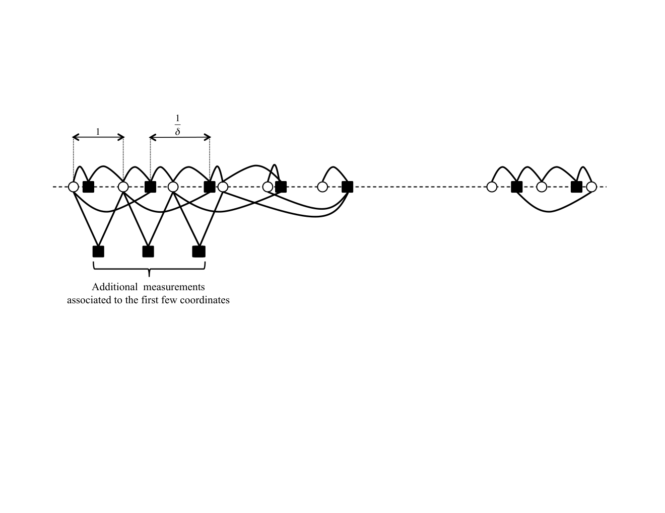
It is convenient to think of the graph structure that they induce on the reconstruction problem. Associate one node (a variable node in the language of factor graphs) to each coordinate ii in the unknown signal xx. Order these nodes on the real line ℝ{\mathbb{R}}, putting the ii-th node at location i∈ℝi\in{\mathbb{R}}. Analogously, associate a node (a factor node) to each coordinate aa in the measurement vector yy, and place the node aa at position a/δa/\delta on the same line. Connect this node to all the variable nodes ii such that Aa​i≠0A_{ai}\neq 0. If AA is band diagonal, only nodes that are placed close enough will be connected by an edge. See Figure 1 for an illustration.

In a spatially coupled matrix, additional measurements are associated to the first few coordinates of xx, say coordinates x1,…,xn0x_{1},\dots,x_{n_{0}} with n0n_{0} much smaller than nn. This has a negligible impact on the overall undersampling ratio as n/n0→∞n/n_{0}\to\infty. Although the overall undersampling remains δ<1\delta<1, the coordinates x1,…,xn0x_{1},\dots,x_{n_{0}} are oversampled. This ensures that these first coordinates are recovered correctly (up to a mean square error of order σ2\sigma^{2}). As the algorithm is iterated, the contribution of these first few coordinates is correctly subtracted from all the measurements, and hence we can effectively eliminate those nodes from the graph. In the resulting graph, the first few variables are effectively oversampled and hence the algorithm will reconstruct their values, up to a mean square error of order σ2\sigma^{2}. As the process is iterated, variables are progressively reconstructed, proceeding from left to right along the node layout.

While the above explains the basic dynamics of AMP reconstruction algorithms under spatial coupling, a careful consideration reveals that this picture leaves open several challenging questions. In particular, why does the overall undersampling factor δ\delta have to exceed d¯​(pX)\overline{d}(p_{X}) for reconstruction to be successful? Our proof is based on a potential function argument. We will prove that there exists a potential function for the AMP algorithm, such that, when δ>d¯​(pX)\delta>\overline{d}(p_{X}), this function has its global minimum close to exact reconstruction. Further, we will prove that, unless this minimum is essentially achieved, AMP can always decrease the function. This technique is different from the one followed in [KRU11] for the LDPC codes over the binary erasure channel, and we think it is of independent interest.
Refer to caption
Figure 1: Graph structure of a spatially coupled matrix. Variable nodes are shown as circle and check nodes are represented by square.

1.5 Further related work

The most closely related earlier work was already discussed above.

More broadly, message passing algorithms for compressed sensing where the object of a number of studies studies, starting with [BSB10]. As mentioned, we will focus on approximate message passing (AMP) as introduced in [DMM09, DMM10]. As shown in [DJM11] these algorithms can be used in conjunction with a rich class of denoisers η⁡(⋅)\eta(\,\cdot\,). A subset of these denoisers arise as posterior mean associated to a prior pXp_{X}. Several interesting examples were studied by Schniter and collaborators [Sch10, Sch11, SPS10], and by Rangan and collaborators [Ran11, KGR11].

Spatial coupling has been the object of growing interest within coding theory over the last few years. The first instance of spatially coupled code ensembles were the convolutional LDPC codes of Felström and Zigangirov [FZ99]. While the excellent performances of such codes had been known for quite some time [SLJZ04], the fundamental reason was not elucidated until recently [KRU11] (see also [LF10]). In particular [KRU11] proved, for communication over the binary erasure channel (BEC), that the thresholds of spatially coupled ensembles under message passing decoding coincide with the thresholds of the base LDPC code under MAP decoding. In particular, this implies that spatially coupled ensembles achieve capacity over the BEC. The analogous statement for general memoryless symmetric channels was first elucidated in [KMRU10] and finally proved in [KRU12]. The paper [HMU10] discusses similar ideas in a number of graphical models.

The first application of spatial coupling ideas to compressed sensing is due to Kudekar and Pfister [KP10]. They consider a class of sparse spatially coupled sensing matrices, very similar to parity check matrices for spatially coupled LDPC codes. On the other hand, their proposed message passing algorithms do not make use of the signal distribution pXp_{X}, and do not fully exploit the potential of spatially coupled matrices. The message passing algorithm used here belongs to the general class introduced in [DMM09]. The specific use of the minimum-mean square error denoiser was suggested in [DMM10]. The same choice is made in [KMS+11], which also considers Gaussian matrices with heteroscedastic entries although the variance structure is somewhat less general.

Finally, let us mention that robust sparse recovery of kk-sparse vectors from m=O⁡(k​log⁡log⁡(n/k))m=O(k\log\log(n/k)) measurement is possible, using suitable ‘adaptive’ sensing schemes [IPW11].

2 Matrix and algorithm construction

In this section, we define an ensemble of random matrices, and the corresponding choices of QtQ^{t}, 𝖻t{\sf b}^{t}, ηt\eta_{t} that achieve the reconstruction guarantees in Theorems 1.6 and 1.7. We proceed by first introducing a general ensemble of random matrices. Correspondingly, we define a deterministic recursion named state evolution, that plays a crucial role in the algorithm analysis. In Section 2.3, we define the algorithm parameters and construct specific choices of QtQ^{t}, 𝖻t{\sf b}^{t}, ηt\eta_{t}. The last section also contains a restatement of Theorems 1.6 and 1.7, in which this construction is made explicit.

2.1 General matrix ensemble

The sensing matrix AA will be constructed randomly, from an ensemble denoted by ℳ⁡(W,M,N){\cal M}(W,M,N). The ensemble depends on two integers M,N∈ℕM,N\in{\mathbb{N}}, and on a matrix with non-negative entries W∈ℝ+𝖱×𝖢W\in{\mathbb{R}}_{+}^{{\sf R}\times{\sf C}}, whose rows and columns are indexed by the finite sets 𝖱{\sf R}, 𝖢{\sf C} (respectively ‘rows’ and ‘columns’). The band-diagonal structure that is characteristic of spatial coupling is imposed by a suitable choice of the matrix WW. In this section we define the ensemble for a general choice of WW. In Section 2.4 we discuss a class of choices for WW that corresponds to spatial coupling, and that yields Theorems 1.6 and 1.7.

In a nutshell, the sensing matrix AA is obtained from WW through a suitable ‘lifting’ procedure. Each entry Wr,cW_{r,c} is replaces my an M×NM\times N block with i.i.d. entries Ai​j∼𝖭⁡(0,Wr,c/M)A_{ij}\sim{\sf N}(0,W_{r,c}/M). Rows and columns of AA are then re-ordered uniformly at random to ensure exchangeability. For the reader familiar with the application of spatial coupling to coding theory, it might be useful to notice the differences and analogies with graph liftings. In that case, the ‘lifted’ matrix is obtained by replacing each edge in the base graph with a random permutation matrix.

Passing to the formal definition, we will assume that the matrix WW is roughly row-stochastic, i.e.,

12≤∑c∈𝖢Wr,c≤2,for all r∈𝖱.\displaystyle\frac{1}{2}\leq\sum_{c\in{\sf C}}W_{r,c}\leq 2\,,\;\;\;\;\;\;\;\mbox{for all }r\in{\sf R}\,. (28)

(This is a convenient simplification for ensuring correct normalization of AA.) We will let |𝖱|≡Lr|{\sf R}|\equiv L_{r} and |𝖢|=Lc|{\sf C}|=L_{c} denote the matrix dimensions. The ensemble parameters are related to the sensing matrix dimensions by n=N​Lcn=NL_{c} and m=M​Lrm=ML_{r}.

In order to describe a random matrix A∼ℳ⁡(W,M,N)A\sim{\cal M}(W,M,N) from this ensemble, partition the columns and row indices in, respectively, LcL_{c} and LrL_{r} groups of equal size. Explicitly

[n]\displaystyle[n] =∪s∈𝖢C(s),|C(s)|=N,\displaystyle=\cup_{s\in{\sf C}}C(s)\,,\;\;\;\;|C(s)|=N\,,
[m]\displaystyle[m] =∪r∈𝖱R(r),|R(r)|=M.\displaystyle=\cup_{r\in{\sf R}}R(r)\,,\;\;\;\;|R(r)|=M\,.

Here and below we use [k][k] to denote the set of first kk integers [k]≡{1,2,…,k}[k]\equiv\{1,2,\dots,k\}. Further, if i∈R⁡(r)i\in R(r) or j∈C⁡(s)j\in C(s) we will write, respectively, r=𝗀⁡(i)r={\sf g}(i) or s=𝗀⁡(j)s={\sf g}(j). In other words 𝗀⁡(⋅){\sf g}(\,\cdot\,) is the operator determining the group index of a given row or column.

With this notation we have the following concise definition of the ensemble.

Definition 2.1.

A random sensing matrix AA is distributed according to the ensemble ℳ⁡(W,M,N){\cal M}(W,M,N) (and we write A∼ℳ⁡(W,M,N)A\sim{\cal M}(W,M,N)) if the partition of rows and columns ([m]=∪r∈𝖱R(r)[m]=\cup_{r\in{\sf R}}R(r) and [n]=∪s∈𝖢C(s)[n]=\cup_{s\in{\sf C}}C(s)) are uniformly random, and given this partitioning, the entries {Ai​j,i∈[m],j∈[n]}\{A_{ij},\;\;i\in[m],j\in[n]\} are independent Gaussian random variables with 77 7 As in many papers on compressed sensing, the matrix here has independent zero-mean Gaussian entries; however, unlike standard practice, here the entries are of widely different variances.

Ai​j∼𝖭⁡(0,1M​W𝗀⁡(i),𝗀⁡(j)).\displaystyle A_{ij}\sim{\sf N}\Big(0,\frac{1}{M}\,W_{{\sf g}(i),{\sf g}(j)}\Big)\,. (29)

We refer to Fig. 2 for an illustration. Note that the randomness of the partitioning of row and column indices is only used in the proof of Lemma 4.1 (cf. [JM12a]), and hence this and other illustrations assume that the partitions are contiguous.

For proving Theorem 1.6 and Theorem 1.7 we will consider suitable sequences of ensembles ℳ⁡(W,M,N){\cal M}(W,M,N) with undersampling ratio converging to δ\delta. While a complete description is given below, let us stress that we take the limit M,N→∞M,N\to\infty (with M=N​δM=N\delta) before the limit Lr,Lc→∞L_{r},L_{c}\to\infty . Hence, the resulting matrix AA is essentially dense: the fraction of non-zero entries per row vanishes only after the number of groups goes to ∞\infty.

W 1 , 1 W 1 , 2 W 1 , 3 W 2 , 1 W 2 , 2 W 2 , 3 W 2 , 4 W 3 , 1 W 3 , 2 W 3 , 3 W 3 , 4 W 3 , 5 W - L r 1 , - L c 3 W - L r 1 , - L c 2 W - L r 1 , - L c 1 W - L r 1 , L c W L r , - L c 2 W L r , - L c 1 W L r , L c

Figure 2: Construction of the spatially coupled measurement matrix AA as described in Section 2.1. The matrix is divided into blocks with size MM by NN. (Number of blocks in each row and each column are respectively Lc{L_{c}} and Lr{L_{r}}, hence m=M​Lrm=M{L_{r}}, n=N​Lcn=N{L_{c}}). The matrix elements Ai​jA_{ij} are chosen as 𝖭⁡(0,1M​W𝗀⁡(i),𝗀⁡(j)){\sf N}(0,\frac{1}{M}W_{{\sf g}(i),{\sf g}(j)}). In this figure, Wi,jW_{i,j} depends only on |i−j||i-j| and thus blocks on each diagonal have the same variance.

2.2 State evolution

State evolution allows an exact asymptotic analysis of AMP algorithms in the limit of a large number of dimensions. As indicated by the name, it bears close resemblance to the density evolution method in iterative coding theory [RU08]. Somewhat surprisingly, this analysis approach is asymptotically exact despite the underlying factor graph being far from locally tree-like.

State evolution was first developed in [DMM09] on the basis of heuristic arguments, and substantial numerical evidence. Subsequently, it was proved to hold for Gaussian sensing matrices with i.i.d. entries, and a broad class of iterative algorithm in [BM11]. These proofs were further generalized in [Ran11], to cover ‘generalized’ AMP algorithms.

In the present case, state evolution takes the following form. 88 8 In previous work, the state variable concerned a single scalar, representing the mean-squared error in the current reconstruction, averaged across all coordinates. In this paper, the dimensionality of the state variable is much larger, because it contains ψ\psi, an individualized MSE for each coordinate of the reconstruction and also ϕ\phi, a noise variance for the residuals rtr^{t} for each measurement coordinate.

Definition 2.2.

Given W∈ℝ+𝖱×𝖢W\in{\mathbb{R}}_{+}^{{\sf R}\times{\sf C}} roughly row-stochastic, and δ>0\delta>0, the corresponding state evolution maps 𝖳W′:ℝ+𝖱→ℝ+𝖢{\sf T}^{\prime}_{W}:{\mathbb{R}}_{+}^{{\sf R}}\to{\mathbb{R}}_{+}^{{\sf C}}, 𝖳W′′:ℝ+𝖢→ℝ+𝖱{\sf T}^{\prime\prime}_{W}:{\mathbb{R}}_{+}^{{\sf C}}\to{\mathbb{R}}_{+}^{{\sf R}}, are defined as follows. For ϕ=(ϕa)a∈𝖱∈ℝ+𝖱\phi=(\phi_{a})_{a\in{\sf R}}\in{\mathbb{R}}_{+}^{{\sf R}}, ψ=(ψi)i∈𝖢∈ℝ+𝖢\psi=(\psi_{i})_{i\in{\sf C}}\in{\mathbb{R}}_{+}^{{\sf C}}, we let:

𝖳W′​(ϕ)i\displaystyle{\sf T}^{\prime}_{W}(\phi)_{i} =\displaystyle= 𝗆𝗆𝗌𝖾⁡(∑b∈𝖱Wb,i​ϕb−1),\displaystyle{\sf mmse}\Big(\sum_{b\in{\sf R}}W_{b,i}\phi_{b}^{-1}\Big)\,, (30)
𝖳W′′​(ψ)a\displaystyle{\sf T}^{\prime\prime}_{W}(\psi)_{a} =\displaystyle= σ2+1δ​∑i∈𝖢Wa,i​ψi.\displaystyle\sigma^{2}+\frac{1}{\delta}\sum_{i\in{\sf C}}W_{a,i}\,\psi_{i}\,. (31)

We finally define 𝖳W=𝖳W′∘𝖳W′′{\sf T}_{W}={\sf T}^{\prime}_{W}\circ{\sf T}^{\prime\prime}_{W}.

In the following, we shall omit the subscripts from 𝖳W{\sf T}_{W} whenever clear from the context.

Definition 2.3.

Given W∈ℝ+Lr×LcW\in{\mathbb{R}}_{+}^{{L_{r}}\times{L_{c}}} roughly row-stochastic, the corresponding state evolution sequence is the sequence of vectors {ϕ⁡(t),ψ⁡(t)}t≥0\{\phi(t),\psi(t)\}_{t\geq 0}, ϕ⁡(t)=(ϕa​(t))a∈𝖱∈ℝ+𝖱\phi(t)=(\phi_{a}(t))_{a\in{\sf R}}\in{\mathbb{R}}_{+}^{{\sf R}}, ψ⁡(t)=(ψi​(t))i∈𝖢∈ℝ+𝖢\psi(t)=(\psi_{i}(t))_{i\in{\sf C}}\in{\mathbb{R}}_{+}^{{\sf C}}, defined recursively by ϕ⁡(t)=𝖳W′′​(ψ⁡(t))\phi(t)={\sf T}^{\prime\prime}_{W}(\psi(t)), ψ⁡(t+1)=𝖳W′​(ϕ⁡(t))\psi(t+1)={\sf T}^{\prime}_{W}(\phi(t)), with initial condition

ψi​(0)=∞​ for all ​i∈𝖢.\displaystyle\psi_{i}(0)=\infty\mbox{ for all }i\in{\sf C}\,. (32)

Hence, for all t≥0t\geq 0,

ϕa​(t)=σ2+1δ​∑i∈𝖢Wa,i​ψi​(t),ψi​(t+1)=𝗆𝗆𝗌𝖾⁡(∑b∈𝖱Wb,i​ϕb​(t)−1).\displaystyle\begin{split}\phi_{a}(t)&=&\sigma^{2}+\frac{1}{\delta}\sum_{i\in{\sf C}}W_{a,i}\,\psi_{i}(t)\,,\\ \psi_{i}(t+1)&=&{\sf mmse}\Big(\sum_{b\in{\sf R}}W_{b,i}\phi_{b}(t)^{-1}\Big)\,.\end{split} (33)

The quantities ψi​(t)\psi_{i}(t), ϕa​(t)\phi_{a}(t) correspond to the asymptotic MSE achieved by the AMP algorithm. More precisely, ψi​(t)\psi_{i}(t) corresponds to the asymptotic mean square error 𝔼⁡{(xjt−xj)2}{\mathbb{E}}\{(x_{j}^{t}-x_{j})^{2}\} for j∈C⁡(i)j\in C(i), as N→∞N\to\infty. Analogously, ϕa​(t)\phi_{a}(t) is the noise variance in residuals rjtr^{t}_{j} corresponding to rows j∈R⁡(a)j\in R(a). This correspondence is stated formally in Lemma 4.1 below. The state evolution (33) describes the evolution of these quantities. In particular, the linear operation in Eq. (7) corresponds to a sum of noise variances as per Eq. (31) and the application of denoisers ηt\eta_{t} corresponds to a noise reduction as per Eq. (30).

As we will see, the definition of denoiser function ηt\eta_{t} involves the state vector ϕ⁡(t)\phi(t). (Notice that the state vectors {ϕ⁡(t),ψ⁡(t)}t≥0\{\phi(t),\psi(t)\}_{t\geq 0} can be precomputed). Hence, ηt\eta_{t} is ‘tuned’ according to the predicted reconstruction error at iteration tt.

2.3 General algorithm definition

In order to fully define the AMP algorithm (6), (7), we need to provide constructions for the matrix QtQ^{t}, the nonlinearities ηt\eta_{t}, and the vector 𝖻t{\sf b}^{t}. In doing this, we exploit the fact that the state evolution sequence {ϕ⁡(t)}t≥0\{\phi(t)\}_{t\geq 0} can be precomputed.

We define the matrix QtQ^{t} by

Qi​jt≡ϕ𝗀⁡(i)​(t)−1∑k=1LrWk,𝗀⁡(j)​ϕk​(t)−1.\displaystyle Q_{ij}^{t}\equiv\frac{\phi_{{\sf g}(i)}(t)^{-1}}{\sum_{k=1}^{{L_{r}}}W_{k,{\sf g}(j)}\phi_{k}(t)^{-1}}\,. (34)

Notice that QtQ^{t} is block-constant: for any r,s∈[L]r,s\in[L], the block QR⁡(r),C⁡(s)tQ^{t}_{R(r),C(s)} has all its entries equal.

As mentioned in Section 1, the function ηt:ℝn→ℝn\eta_{t}:{\mathbb{R}}^{n}\to{\mathbb{R}}^{n} is chosen to be separable, i.e., for v∈ℝNv\in{\mathbb{R}}^{N}:

ηt​(v)=(ηt,1​(v1),ηt,2​(v2),…,ηt,N​(vN)).\displaystyle\eta_{t}(v)=\big(\eta_{t,1}(v_{1}),\eta_{t,2}(v_{2}),\;\dots\;,\eta_{t,N}(v_{N})\big)\,. (35)

We take ηt,i\eta_{t,i} to be a conditional expectation estimator for X∼pXX\sim p_{X} in gaussian noise:

ηt,i(vi)=𝔼{X|X+s𝗀⁡(i)(t)−1/2Z=vi},sr(t)≡∑u∈𝖱Wu,rϕu(t)−1.\displaystyle\eta_{t,i}(v_{i})={\mathbb{E}}\big\{X\,\big|\,X+\,s_{{\sf g}(i)}(t)^{-1/2}Z=v_{i}\,\big\}\,,\;\;\;\;s_{r}(t)\equiv\sum_{u\in{\sf R}}W_{u,r}\phi_{u}(t)^{-1}\,. (36)

Notice that the function ηt,i​(⋅)\eta_{t,i}(\,\cdot\,) depends on ii only through the group index 𝗀⁡(i){\sf g}(i), and in fact only parametrically through s𝗀⁡(i)​(t)s_{{\sf g}(i)}(t). It is also interesting to notice that the denoiser ηt,i​(⋅)\eta_{t,i}(\,\cdot\,) does not have any tuning parameter to be optimized over. This was instead the case for the soft-thresholding AMP algorithm studied in [DMM09] for which the threshold level had to be adjusted in a non-trivial manner to the sparsity level. This difference is due to the fact that the prior pXp_{X} is assumed to be known and hence the optimal denoiser is uniquely determined to be the posterior expectation as per Eq. (36).

Finally, in order to define the vector 𝖻it{\sf b}^{t}_{i}, let us introduce the quantity

⟨ηt′⟩u=1N​∑i∈C⁡(u)ηt,i′​(xit+((Qt⊙A)∗​rt)i).\displaystyle\langle\eta^{\prime}_{t}\rangle_{u}=\frac{1}{N}\sum_{i\in C(u)}\eta^{\prime}_{t,i}\big(x^{t}_{i}+((Q^{t}\odot A)^{*}r^{t})_{i}\big)\,. (37)

The vector 𝖻t{\sf b}^{t} is then defined by

𝖻it≡1δ​∑u∈𝖢W𝗀⁡(i),u​Q~𝗀⁡(i),ut−1​⟨ηt−1′⟩u,\displaystyle{\sf b}^{t}_{i}\equiv\frac{1}{\delta}\sum_{u\in{\sf C}}W_{{\sf g}(i),u}\widetilde{Q}^{t-1}_{{\sf g}(i),u}\,\langle\eta^{\prime}_{t-1}\rangle_{u}\,, (38)

where we defined Qi,jt=Q~r,utQ^{t}_{i,j}=\widetilde{Q}^{t}_{r,u} for i∈R⁡(r)i\in R(r), j∈C⁡(u)j\in C(u). Again 𝖻it{\sf b}^{t}_{i} is block-constant: the vector 𝖻C⁡(u)t{\sf b}^{t}_{C(u)} has all its entries equal.

This completes our definition of the AMP algorithm. Let us conclude with a few computational remarks:

  1. 1.

    The quantities Q~t\tilde{Q}^{t}, ϕ⁡(t)\phi(t) can be precomputed efficiently iteration by iteration, because they are, respectively, Lr×Lc{L_{r}}\times{L_{c}} and Lr{L_{r}}-dimensional, and, as discussed further below, Lr,Lc{L_{r}},{L_{c}} are much smaller than m,nm,n. The most complex part of this computation is implementing the iteration (33), which has complexity O⁡((Lr+Lc)3)O(({L_{r}}+{L_{c}})^{3}), plus the complexity of evaluating the 𝗆𝗆𝗌𝖾{\sf mmse} function, which is a one-dimensional integral.

  2. 2.

    The vector 𝖻t{\sf b}^{t} is also block-constant, so can be efficiently computed using Eq. (38).

  3. 3.

    Instead of computing ϕ⁡(t)\phi(t) analytically by iteration (33), ϕ⁡(t)\phi(t) can also be estimated from data xt,rtx^{t},r^{t}. In particular, by generalizing the methods introduced in [DMM09, Mon12], we get the estimator

    ϕ^a​(t)=1M​‖rR⁡(a)t‖22,\displaystyle\widehat{\phi}_{a}(t)=\frac{1}{M}\,\|r^{t}_{R(a)}\|^{2}_{2}\,, (39)

    where rR⁡(a)t=(rjt)j∈R⁡(a)r^{t}_{R(a)}=(r^{t}_{j})_{j\in R(a)} is the restriction of rtr^{t} to the indices in R⁡(a)R(a). An alternative more robust estimator (more resilient to outliers), would be

    ϕ^a​(t)1/2=1Φ−1​(3/4)​|rR⁡(a)t|(M/2),\displaystyle\widehat{\phi}_{a}(t)^{1/2}=\frac{1}{\Phi^{-1}(3/4)}\,|r^{t}_{R(a)}|_{(M/2)}\,, (40)

    where Φ⁡(z)\Phi(z) is the Gaussian distribution function, and, for v∈ℝKv\in{\mathbb{R}}^{K}, |v|(ℓ)|v|_{(\ell)} is the ℓ\ell-th largest entry in the vector (|v1|,|v2|,…,|vK|)(|v_{1}|,|v_{2}|,\dots,|v_{K}|). (See, e.g., [HR09] for background in robust estimation.) The idea underlying both of the above estimators is that the components of rR⁡(a)tr^{t}_{R(a)} are asymptotically i.i.d. with mean zero and variance ϕa​(t)\phi_{a}(t).

2.4 Choices of parameters, and spatial coupling

In order to prove our main Theorem 1.6, we use a sensing matrix from the ensemble ℳ⁡(W,M,N){\cal M}(W,M,N) for a suitable choice of the matrix W∈ℝ𝖱×𝖢W\in{\mathbb{R}}^{{\sf R}\times{\sf C}}. Our construction depends on parameters ρ∈ℝ+\rho\in{\mathbb{R}}_{+}, L,L0∈ℕL,L_{0}\in{\mathbb{N}}, and on the ‘shape function’ 𝒲{\cal W}. As explained below, ρ\rho will be taken to be small, and hence we will treat 1/ρ1/\rho as an integer to avoid rounding (which introduces in any case a negligible error).

Here and below ≅\cong denotes identity between two sets up to a relabeling.

Definition 2.4.

A shape function is a function 𝒲:ℝ→ℝ+{\cal W}:{\mathbb{R}}\to{\mathbb{R}}_{+} continuously differentiable, with support in [−1,1][-1,1] and such that ∫ℝ𝒲⁡(u)​𝑑u=1\int_{\mathbb{R}}{\cal W}(u)\,{\rm d}u=1, and 𝒲⁡(−u)=𝒲⁡(u){\cal W}(-u)={\cal W}(u).

We let 𝖢≅{−2​ρ−1,…,0,1,…,L−1}{\sf C}\cong\{-2\rho^{-1},\dots,0,1,\dots,L-1\}, so that Lc=L+2​ρ−1{L_{c}}=L+2\rho^{-1}. Also let 𝖢0={0,1,…,L−1}{\sf C}_{0}=\{0,1,\dotsc,L-1\}.

The rows are partitioned as follows:

𝖱=𝖱0∪{∪i=−2​ρ−1−1𝖱i},\displaystyle{\sf R}={\sf R}_{0}\cup\Big\{\cup_{i=-2\rho^{-1}}^{-1}{\sf R}_{i}\Big\}\,,

where 𝖱0≅{−ρ−1,…,0,1,…,L−1+ρ−1}{\sf R}_{0}\cong\{-\rho^{-1},\dots,0,1,\dots,L-1+\rho^{-1}\}, and 𝖱i={i​L0,…,(i+1)​L0−1}{\sf R}_{i}=\{i{L_{0}},\dotsc,(i+1){L_{0}}-1\}, for i=−2​ρ−1,…,−1i=-2\rho^{-1},\dotsc,-1. Hence, |𝖱i|=L0|{\sf R}_{i}|=L_{0}, and Lr=Lc+2​ρ−1​L0{L_{r}}={L_{c}}+2\rho^{-1}{L_{0}}.

Finally, we take NN so that n=N​Lcn=N{L_{c}}, and let M=N​δM=N\delta so that m=M​Lr=N⁡(Lc+2​ρ−1​L0)​δm=M{L_{r}}=N({L_{c}}+2\rho^{-1}{L_{0}})\delta. Notice that m/n=δ⁡(Lc+2​ρ−1​L0)/Lcm/n=\delta({L_{c}}+2\rho^{-1}{L_{0}})/{L_{c}}. Since we will take Lc{L_{c}} much larger than L0/ρL_{0}/\rho, we in fact have m/nm/n arbitrarily close to δ\delta.

Given these inputs, we construct the corresponding matrix W=W⁡(L,L0,𝒲,ρ)W=W(L,L_{0},{\cal W},\rho) as follows.

  1. 1.

    For i∈{−2​ρ−1,…,−1}i\in\{-2\rho^{-1},\dots,-1\}, and each a∈𝖱ia\in{\sf R}_{i}, we let Wa,i=1W_{a,i}=1. Further, Wa,j=0W_{a,j}=0 for all j∈𝖢∖{i}j\in{\sf C}\setminus\{i\}.

  2. 2.

    For all a∈𝖱0≅{−ρ−1,…,0,…,L−1+ρ−1}a\in{\sf R}_{0}\cong\{-\rho^{-1},\dots,0,\dots,L-1+\rho^{-1}\}, we let

    Wa,i=ρ​𝒲​(ρ⁡(a−i))\displaystyle W_{a,i}=\rho\,{\cal W}\big(\rho\,(a-i)\big)\, i∈{−2​ρ−1,…,L−1}.\displaystyle i\in\{-2\rho^{-1},\dots,L-1\}. (41)
Refer to caption + L ⁢ 2 ρ - 1 ⁢ 2 ρ - 1 L 0 L 0 ⁢ 2 ρ - 1 L R - ⁢ 2 ρ - 1 R - 1 R 0 C 0 C R ⁢ ρ 𝒲 ( ρ ( - a i ) )
Figure 3: Matrix W. The shaded region indicates the non zero entries in the lower part of the matrix. As shown (the lower part of ) the matrix WW is band diagonal.

The role of the rows in {∪i=−2​ρ−1−1𝖱i}\Big\{\cup_{i=-2\rho^{-1}}^{-1}{\sf R}_{i}\Big\} and the corresponding rows in AA are to oversample the first few (namely the first 2​ρ−1​N2\rho^{-1}N) coordinates of the signal as explained in Section 1.4. Furthermore, the restriction of WW to the rows in 𝖱0{\sf R}_{0} is band diagonal as 𝒲{\cal W} is supported on [−1,1][-1,1]. See Fig. 3 for an illustration of the matrix WW.

In the following we occasionally use the shorthand Wa−i≡ρ​𝒲​(ρ⁡(a−i))W_{a-i}\equiv\rho\,{\cal W}\big(\rho\,(a-i)\big). Note that WW is roughly row-stochastic. Also, the restriction of WW to the rows in 𝖱0{\sf R}_{0} is roughly column-stochastic. This follows from the fact that the function 𝒲⁡(⋅){\cal W}(\cdot) has continuous (and thus bounded) derivative on the compact interval [−1,1][-1,1], and ∫ℝ𝒲⁡(u)​𝑑u=1\int_{{\mathbb{R}}}{\cal W}(u){\rm d}u=1. Therefore, using the standard convergence of Riemann sums to Riemann integrals and the fact that ρ\rho is small, we get the result.

We are now in position to restate Theorem 1.6 in a more explicit form.

Theorem 2.5.

Let pXp_{X} be a probability measure on the real line with δ>d¯​(pX)\delta>\overline{d}(p_{X}), and let 𝒲:ℝ→ℝ+{\cal W}:{\mathbb{R}}\to{\mathbb{R}}_{+} be a shape function. For any ε>0{\varepsilon}>0, there exist L0,L,ρL_{0},L,\rho, t0t_{0}, σ02=σ0​(ε,δ,pX)2\sigma_{0}^{2}=\sigma_{0}({\varepsilon},\delta,p_{X})^{2} such that L0/(L​ρ)≤εL_{0}/(L\rho)\leq{\varepsilon}, and further the following holds true for W=W⁡(L,L0,𝒲,ρ)W=W(L,L_{0},{\cal W},\rho).

For N≥0N\geq 0, and A⁡(n)∼ℳ⁡(W,M,N)A(n)\sim{\cal M}(W,M,N) with M=N​δM=N\delta, and for all σ2≤σ02\sigma^{2}\leq\sigma_{0}^{2}, t≥t0t\geq t_{0}, we almost surely have

lim​supN→∞​1n​‖xt​(A⁡(n),y⁡(n))−x⁡(n)‖2≤ε.\displaystyle\underset{N\to\infty}{\rm{lim\,sup}}\frac{1}{n}\big\|x^{t}\big(A(n);y(n)\big)-x(n)\big\|^{2}\leq{\varepsilon}\,. (42)

Further, under the same assumptions, we have

lim​supN→∞​1n​𝔼​{‖xt​(A⁡(n),y⁡(n))−x⁡(n)‖2}≤ε.\displaystyle\underset{N\to\infty}{\rm{lim\,sup}}\frac{1}{n}{\mathbb{E}}\big\{\big\|x^{t}\big(A(n);y(n)\big)-x(n)\big\|^{2}\big\}\leq{\varepsilon}\,. (43)

In order to obtain a stronger form of robustness, as per Theorem 1.7, we slightly modify the sensing scheme. We construct the sensing matrix A~\tilde{A} from AA by appending 2​ρ−1​L02\rho^{-1}L_{0} rows in the bottom.

A~=(A0I),\displaystyle\tilde{A}=\begin{pmatrix}\quad\quad A\\ \hline\cr\lx@intercol\hfil 0\hfil\lx@intercol\vrule\lx@intercol&I\end{pmatrix}, (44)

where II is the identity matrix of dimensions 2​ρ−1​L02\rho^{-1}L_{0}. Note that this corresponds to increasing the number of measurements; however, the asymptotic undersampling rate remains δ\delta, provided that L0/(L​ρ)→0L_{0}/(L\rho)\to 0, as n→∞n\to\infty.

The reconstruction scheme is modified as follows. Let x1x_{1} be the vector obtained by restricting xx to entries in ∪iC(i)\cup_{i}C(i), where i∈{−2​ρ−1,⋯,L−2​ρ−1−1}i\in\{-2\rho^{-1},\cdots,L-2\rho^{-1}-1\}. Also, let x2x_{2} be the vector obtained by restricting xx to entries in ∪iC(i)\cup_{i}C(i), where i∈{L−2​ρ−1,⋯,L−1}i\in\{L-2\rho^{-1},\cdots,L-1\}. Therefore, x=(x1,x2)Tx=(x_{1},x_{2})^{T}. Analogously, let y=(y1,y2)Ty=(y_{1},y_{2})^{T} where y1y_{1} is given by the restriction of yy to ∪i∈𝖱R(i)\cup_{i\in{\sf R}}R(i) and y2y_{2} corresponds to the additional 2​ρ−1​L02\rho^{-1}L_{0} rows. Define w1w_{1} and w2w_{2} from the noise vector ww, analogously. Hence,

(y1y2)=(A0I)​(x1x2)+(w1w2).\displaystyle\begin{pmatrix}y_{1}\\ y_{2}\end{pmatrix}=\begin{pmatrix}\quad\quad A\\ \hline\cr\lx@intercol\hfil 0\hfil\lx@intercol\vrule\lx@intercol&I\end{pmatrix}\begin{pmatrix}x_{1}\\ x_{2}\end{pmatrix}+\begin{pmatrix}w_{1}\\ w_{2}\end{pmatrix}. (45)

Note that the sampling rate for vector x2x_{2} is one, i.e., y2y_{2} and x2x_{2} are of the same length and are related to each other through the identity matrix II. Hence, we have a fairly good approximation of these entries. We use the AMP algorithm as described in the previous section to obtain an estimation of x1x_{1}. Formally, let xtx^{t} be the estimation at iteration tt obtained by applying the AMP algorithm to the problem y1=A​x+w1y_{1}=Ax+w_{1}. The modified estimation is then x~t=(x1t,y2)T\tilde{x}^{t}=(x_{1}^{t},y_{2})^{T}.

As we will see later, this modification in the sensing matrix and algorithm, while not necessary, simplifies some technical steps in the proof.

Theorem 2.6.

Let pXp_{X} be a probability measure on the real line with δ>D¯​(pX)\delta>\overline{D}(p_{X}), and let 𝒲:ℝ→ℝ+{\cal W}:{\mathbb{R}}\to{\mathbb{R}}_{+} be a shape function. There exist L0,L,ρL_{0},L,\rho, t0t_{0} and a finite stability constant C=C⁡(pX,δ)C=C(p_{X},\delta), such that L0/(L​ρ)<εL_{0}/(L\rho)<{\varepsilon}, for any given ε>0{\varepsilon}>0, and the following holds true for the modified reconstruction scheme.

For t≥t0t\geq t_{0}, we almost surely have,

lim​supN→∞​1n​‖x~t​(A~​(n),y⁡(n))−x⁡(n)‖2≤C​σ2.\displaystyle\underset{N\to\infty}{\rm{lim\,sup}}\frac{1}{n}\big\|\tilde{x}^{t}\big(\tilde{A}(n);y(n)\big)-x(n)\big\|^{2}\leq C\sigma^{2}. (46)

Further, under the same assumptions, we have

lim​supN→∞​1n​𝔼​{‖x~t​(A~​(n),y⁡(n))−x⁡(n)‖2}≤C​σ2.\displaystyle\underset{N\to\infty}{\rm{lim\,sup}}\frac{1}{n}{\mathbb{E}}\big\{\big\|\tilde{x}^{t}\big(\tilde{A}(n);y(n)\big)-x(n)\big\|^{2}\big\}\leq C\sigma^{2}. (47)

Finally, in the asymptotic case where ℓ=L​ρ→∞\ell=L\rho\to\infty, ρ→0\rho\to 0, L0→∞{L_{0}}\to\infty, we have

limσ→01σ2​{limt→∞lim​supN→∞​1n​‖x~t​(A~​(n),y⁡(n))−x⁡(n)‖2}≤4​δ−2​D¯​(pX)δ−D¯​(pX).\lim_{\sigma\to 0}\frac{1}{\sigma^{2}}\Big\{\lim_{t\to\infty}\underset{N\to\infty}{\rm{lim\,sup}}\frac{1}{n}\big\|\tilde{x}^{t}\big(\tilde{A}(n);y(n)\big)-x(n)\big\|^{2}\Big\}\leq\frac{4\delta-2\overline{D}(p_{X})}{\delta-\overline{D}(p_{X})}\,.

It is obvious that Theorems 2.5 and 2.6 respectively imply Theorems 1.6 and 1.7. We shall therefore focus on the proofs of Theorems 2.5 and 2.6 in the rest of the paper.

Notice that the results of Theorems 2.5 and 2.6 only deal with a linear subsequence n=N​Lcn=N{L_{c}} with N→∞N\to\infty. However, this is sufficient to prove the claim of Theorems 1.6 and 1.7. More specifically, suppose that nn is not a multiple of Lc{L_{c}}. Let n′n^{\prime} be the smallest number greater than nn which is divisible by Lc{L_{c}}, i.e., n′=⌈n/Lc⌉​Lcn^{\prime}=\lceil n/{L_{c}}\rceil{L_{c}}, and let x^=(x,0)T∈ℝn′\hat{x}=(x,0)^{T}\in{\mathbb{R}}^{n^{\prime}} be obtained by padding xx with zeros. Let x^t\hat{x}^{t} denote the Bayes optimal AMP estimate of x^\hat{x} and xtx^{t} be the restriction of x^t\hat{x}^{t} to the first nn entries. We have (1/n)​‖xt−x‖2≤(n′/n)​(1/n′)​‖x^t−x^‖2(1/n)\|x^{t}-x\|^{2}\leq(n^{\prime}/n)(1/n^{\prime})\|\hat{x}^{t}-\hat{x}\|^{2}. The result of Theorem 1.6 follows by applying Theorem 2.5 (for the sequence n=N​Lcn=N{L_{c}}, N→∞N\to\infty), and noting that n′/n≤(1+Lc/n)→1n^{\prime}/n\leq(1+{L_{c}}/n)\to 1, as N→∞N\to\infty. Similar comment applies to Theorems 2.6 and 1.7.

3 Advantages of spatial coupling

Within the construction proposed in this paper, spatially coupled sensing matrices have independent heteroscedastic entries (entries with different variances). In addition to this, we also oversample a few number of coordinates of the signal, namely the first 2​ρ−1​N2\rho^{-1}N coordinates. In this section we informally discuss the various components of this scheme.

It can be instructive to compare this construction with the case of homoscedastic Gaussian matrices (i.i.d. entries). For the reader familiar with coding theory, this comparison is analogous to the comparison between regular LDPC codes and spatially coupled regular LDPC codes. Regular LDPC codes have been known since Gallager [Gal63, MMRU09] to achieve the channel capacity, as the degree gets large, under maximum likelihood decoding. However their performances under practical (belief propagation) decoding is rather poor. When the code ensemble is modified via spatial coupling, the belief propagation performances improve to become asymptotically equivalent to the maximum likelihood performances. Hence spatially coupled LDPC codes achieve capacity under practical decoding schemes.

Similarly, standard (non-spatially coupled) sensing matrices achieve the information theoretic limit under computationally unpractical recovery schemes [WV10], but do not perform ideally under practical reconstruction algorithms. Consider for instance Bayes optimal AMP. Within the standard ensemble, the state evolution recursion reads

ϕ⁡(t)=σ2+1δ​ψ​(t),ψ⁡(t+1)=𝗆𝗆𝗌𝖾⁡(ϕ​(t)−1).\displaystyle\begin{split}\phi(t)&=\sigma^{2}+\frac{1}{\delta}\psi(t)\,,\\ \psi(t+1)&={\sf mmse}\big(\phi(t)^{-1}\big)\,.\end{split} (48)

Let δ~​(pX)≡sups≥0s⋅𝗆𝗆𝗌𝖾⁡(s)>d¯​(pX)\tilde{\delta}(p_{X})\equiv\sup_{s\geq 0}s\cdot{\sf mmse}(s)>\overline{d}(p_{X}). It is immediate to see that the last recursion develops two (or possibly more) stable fixed points for δ<δ~​(pX)\delta<\tilde{\delta}(p_{X}) and all σ2\sigma^{2} small enough. The smallest fixed point, call it ϕgood\phi_{\rm good}, corresponds to correct reconstruction and is such that ϕgood=O⁡(σ2)\phi_{\rm good}=O(\sigma^{2}) as σ→0\sigma\to 0. The largest fixed point, call it ϕbad\phi_{\rm bad}, corresponds to incorrect reconstruction and is such that ϕbad=Θ⁡(1)\phi_{\rm bad}=\Theta(1) as σ→0\sigma\to 0. A study of the above recursion shows that limt→∞ϕ⁡(t)=ϕbad\lim_{t\to\infty}\phi(t)=\phi_{\rm bad}. State evolution converges to the ‘incorrect’ fixed point, hence predicting a large MSE for AMP.

On the contrary, for d¯​(pX)<δ<δ~​(pX)\overline{d}(p_{X})<\delta<\tilde{\delta}(p_{X}) the recursion (48) converges (for appropriate choices of WW as in the previous section) to the ‘ideal’ fixed point limt→∞ϕa​(t)=ϕgood\lim_{t\to\infty}\phi_{a}(t)=\phi_{\rm good} for all aa (except possibly those near the boundaries). This is illustrated in Fig. 4. We also refer to [HMU10] for a survey of examples of the same phenomenon and to [KMS+11, JM12b] for further discussion in compressed sensing.

The above discussion also clarifies why the posterior expectation denoiser is useful. Spatially coupled sensing matrices do not yield better performances than the ones dictated by the best fixed point in the ‘standard’ recursion (48). In particular, replacing the Bayes optimal denoiser by another denoiser ηt\eta_{t} amounts, roughly, to replacing 𝗆𝗆𝗌𝖾{\sf mmse} in Eq. (48) by the MSE of another denoiser, hence leading to worse performances.

In particular, if the posterior expectation denoiser is replaced by soft thresholding, the resulting state evolution recursion always has a unique stable fixed point for homoscedastic matrices [DMM09]. This suggests that spatial coupling does not lead to any improvement for soft thresholding AMP and hence (via the correspondence of [BM12]) for LASSO or ℓ1\ell_{1} reconstruction. This expectation is indeed confirmed numerically in [JM12b].

4 Key lemmas and proof of the main theorems

Our proof is based in a crucial way on state evolution. This effectively reduces the analysis of the algorithm (6), (7) to the analysis of the deterministic recursion (33).

Lemma 4.1.

Let W∈ℝ+𝖱×𝖢W\in{\mathbb{R}}_{+}^{{\sf R}\times{\sf C}} be a roughly row-stochastic matrix (see Eq. (28))and ϕ⁡(t)\phi(t), QtQ^{t}, 𝖻t{\sf b}^{t} be defined as in Section 2.3. Let M=M⁡(N)M=M(N) be such that M/N→δM/N\to\delta, as N→∞N\to\infty. Define m=M​Lrm=M{L_{r}}, n=N​Lcn=N{L_{c}}, and for each N≥1N\geq 1, let A⁡(n)∼ℳ⁡(W,M,N)A(n)\sim{\cal M}(W,M,N). Let {(x⁡(n),w⁡(n))}n≥0\{(x(n),w(n))\}_{n\geq 0} be a converging sequence of instances with parameters (pX,σ2)(p_{X},\sigma^{2}). Then, for all t≥1t\geq 1, almost surely we have

lim​supN→∞​1N​‖xC⁡(i)t​(A⁡(n),y⁡(n))−xC⁡(i)‖22=𝗆𝗆𝗌𝖾⁡(∑a∈𝖱Wa,i​ϕa​(t−1)−1).\displaystyle\underset{N\to\infty}{\rm{lim\,sup}}\frac{1}{N}\|x^{t}_{C(i)}(A(n);y(n))-x_{C(i)}\|_{2}^{2}={\sf mmse}\Big(\sum_{a\in{\sf R}}W_{a,i}\phi_{a}(t-1)^{-1}\Big)\,. (49)

for all i∈𝖢i\in{\sf C}.

This lemma is a straightforward generalization of [BM11]. Since a formal proof does not require new ideas, but a significant amount of new notations, it is presented in a separate publication [JM12a] which covers an even more general setting. In the interest of self-containedness, and to develop useful intuition on state evolution, we present an heuristic derivation of the state evolution equations (33) in Section 6.

The next Lemma provides the needed analysis of the recursion (33).

Lemma 4.2.

Let δ>0\delta>0, and pXp_{X} be a probability measure on the real line. Let 𝒲:ℝ→ℝ+{\cal W}:{\mathbb{R}}\to{\mathbb{R}}_{+} be a shape function.

(a)(a) If δ>d¯​(pX)\delta>\overline{d}(p_{X}), then for any ε>0{\varepsilon}>0, there exist σ0=σ0​(ε,δ,pX),ρ,L∗>0\sigma_{0}=\sigma_{0}({\varepsilon},\delta,p_{X}),\rho,L_{*}>0, such that for any σ2∈[0,σ02],L0>3/δ\sigma^{2}\in[0,\sigma_{0}^{2}],L_{0}>3/\delta, and L>L∗L>L_{*}, the following holds for W=W⁡(L,L0,𝒲,ρ)W=W(L,L_{0},{\cal W},\rho):

limt→∞1L​∑a=−ρ−1L+ρ−1−1ϕa​(t)≤ε.\displaystyle\lim_{t\to\infty}\frac{1}{L}\sum_{a=-\rho^{-1}}^{L+\rho^{-1}-1}\phi_{a}(t)\leq{\varepsilon}. (50)

(b)(b) If further δ>D¯​(pX)\delta>\overline{D}(p_{X}), then there exist ρ,L∗>0\rho,L_{*}>0, and a finite stability constant C=C⁡(pX,δ)C=C(p_{X},\delta), such that for L0>3/δL_{0}>3/\delta, and L>L∗L>L_{*}, the following holds for W=W⁡(L,L0,𝒲,ρ)W=W(L,L_{0},{\cal W},\rho).

limt→∞1L​∑a=−ρ−1L−ρ−1−1ϕa​(t)≤C​σ2.\displaystyle\lim_{t\to\infty}\frac{1}{L}\sum_{a=-\rho^{-1}}^{L-\rho^{-1}-1}\phi_{a}(t)\leq C\sigma^{2}. (51)

Finally, in the asymptotic case where ℓ=L​ρ→∞\ell=L\rho\to\infty, ρ→0\rho\to 0, L0→∞{L_{0}}\to\infty, we have

limσ→0limt→∞1σ2​L​∑a=−ρ−1L−ρ−1−1ϕa​(t)≤3​δ−D¯​(pX)δ−D¯​(pX).\displaystyle\lim_{\sigma\to 0}\lim_{t\to\infty}\frac{1}{\sigma^{2}\,L}\sum_{a=-\rho^{-1}}^{L-\rho^{-1}-1}\phi_{a}(t)\leq\frac{3\delta-\overline{D}(p_{X})}{\delta-\overline{D}(p_{X})}\,. (52)

The proof of this lemma is deferred to Section 7 and is indeed the technical core of the paper.

Now, we have in place all we need to prove our main results.

Proof (Theorem 2.5).

Recall that 𝖢≅{−2ρ−1⋯,L−1}{\sf C}\cong\{-2\rho^{-1}\cdots,L-1\}. Therefore,

lim​supN→∞​1n​‖xt​(A⁡(n),y⁡(n))−x⁡(n)‖2≤1Lc​∑i∈𝖢lim​supN→∞​1N​‖xC⁡(i)t​(A⁡(n),y⁡(n))−xC⁡(i)​(n)‖2≤(a)1Lc​∑i=−2​ρ−1L−1𝗆𝗆𝗌𝖾⁡(∑a∈𝖱Wa,i​ϕa​(t−1)−1)≤(b)1Lc​∑i=−2​ρ−1L−1𝗆𝗆𝗌𝖾⁡(∑a∈𝖱0Wa,i​ϕa​(t−1)−1)≤(c)1Lc​∑i=−2​ρ−1L−1𝗆𝗆𝗌𝖾⁡(12​ϕi+ρ−1​(t−1)−1)≤(d)1Lc​∑a=−ρ−1L+ρ−1−12​ϕa​(t−1).\displaystyle\begin{split}\underset{N\to\infty}{\rm{lim\,sup}}\frac{1}{n}\big\|x^{t}\big(A(n);y(n)\big)-x(n)\big\|^{2}&\leq\frac{1}{{L_{c}}}\sum_{i\in{\sf C}}\underset{N\to\infty}{\rm{lim\,sup}}\frac{1}{N}\big\|x^{t}_{C(i)}\big(A(n);y(n)\big)-x_{C(i)}(n)\big\|^{2}\\ &\stackrel{{\scriptstyle(a)}}{{\leq}}\frac{1}{{L_{c}}}\sum_{i=-2\rho^{-1}}^{L-1}{\sf mmse}\left(\sum_{a\in{\sf R}}W_{a,i}\phi_{a}(t-1)^{-1}\right)\\ &\stackrel{{\scriptstyle(b)}}{{\leq}}\frac{1}{{L_{c}}}\sum_{i=-2\rho^{-1}}^{L-1}{\sf mmse}\left(\sum_{a\in{\sf R}_{0}}W_{a,i}\phi_{a}(t-1)^{-1}\right)\\ &\stackrel{{\scriptstyle(c)}}{{\leq}}\frac{1}{{L_{c}}}\sum_{i=-2\rho^{-1}}^{L-1}{\sf mmse}\left(\frac{1}{2}\phi_{i+\rho^{-1}}(t-1)^{-1}\right)\\ &\stackrel{{\scriptstyle(d)}}{{\leq}}\frac{1}{{L_{c}}}\sum_{a=-\rho^{-1}}^{L+\rho^{-1}-1}2\phi_{a}(t-1).\end{split} (53)

Here, (a)(a) follows from Lemma 4.1; (b)(b) follows from the fact that 𝗆𝗆𝗌𝖾{\sf mmse} is non-increasing; (c) holds because of the following facts: (i)(i) ϕa​(t)\phi_{a}(t) is nondecreasing in aa for every tt (see Lemma 7.10 below). (i​i)(ii) Restriction of WW to the rows in 𝖱0{\sf R}_{0} is roughly column-stochastic. (i​i​i)(iii) 𝗆𝗆𝗌𝖾{\sf mmse} is non-increasing; (d)(d) follows from the inequality 𝗆𝗆𝗌𝖾⁡(s)≤1/s{\sf mmse}(s)\leq 1/s. The result is immediate due to Lemma 4.2, Part (a)(a).

Now, we prove the claim regarding the expected error. Let fn=1n​‖xt​(A⁡(n),y⁡(n))−x⁡(n)‖2f_{n}=\frac{1}{n}\|x^{t}(A(n);y(n))-x(n)\|^{2}. Since limsupn→∞​fn≤ε\underset{n\to\infty}{\lim\sup}\,f_{n}\leq{\varepsilon}, there exists n0n_{0} such that fn≤2​εf_{n}\leq 2{\varepsilon} for n≥n0n\geq n_{0}. Applying reverse Fatou’s lemma to the bounded sequence {fn}n≥n0\{f_{n}\}_{n\geq n_{0}}, we have limsupN→∞​𝔼​fn≤𝔼⁡[limsupN→∞​fn]≤ε\underset{N\to\infty}{\lim\sup}\,{\mathbb{E}}f_{n}\leq{\mathbb{E}}[\underset{N\to\infty}{\lim\sup}\,f_{n}]\leq{\varepsilon}. ∎

Proof (Theorem 2.6).

The proof proceeds in a similar manner to the proof of Theorem 2.5.

lim​supN→∞​1n|x~t​(A~​(n)CLOSE;y(n))−x(n)∥2≤1Lc​{∑i=−2​ρ−1L−2​ρ−1−1lim​supN→∞​1N​‖xC⁡(i)t​(A⁡(n),y⁡(n))−xC⁡(i)​(n)‖2+limN→∞1N​‖w2​(n)‖2}≤1Lc​{∑i=−2​ρ−1L−2​ρ−1−1𝗆𝗆𝗌𝖾⁡(∑a∈𝖱Wa,i​ϕa​(t−1)−1)+limN→∞1N​‖w2​(n)‖2}≤1Lc​{∑i=−2​ρ−1L−2​ρ−1−1𝗆𝗆𝗌𝖾⁡(∑a∈𝖱0Wa,i​ϕa​(t−1)−1)+limN→∞1N​‖w2​(n)‖2}≤1Lc​{∑i=−2​ρ−1L−2​ρ−1−1𝗆𝗆𝗌𝖾⁡(12​ϕi+ρ−1​(t−1)−1)+limN→∞1N​‖w2​(n)‖2}≤1Lc​{∑a=−ρ−1L−ρ−1−12​ϕa​(t−1)+limN→∞1N​‖w2​(n)‖2}≤C​σ2,\displaystyle\begin{split}\underset{N\to\infty}{\rm{lim\,sup}}\frac{1}{n}\big\|\tilde{x}^{t}\big(\tilde{A}(n)&;y(n)\big)-x(n)\big\|^{2}\\ &\leq\frac{1}{{L_{c}}}\Big\{\sum_{i=-2\rho^{-1}}^{L-2\rho^{-1}-1}\underset{N\to\infty}{\rm{lim\,sup}}\frac{1}{N}\big\|x^{t}_{C(i)}\big(A(n);y(n)\big)-x_{C(i)}(n)\big\|^{2}+\lim_{N\to\infty}\frac{1}{N}\big\|w_{2}(n)\big\|^{2}\Big\}\\ &\leq\frac{1}{{L_{c}}}\Big\{\sum_{i=-2\rho^{-1}}^{L-2\rho^{-1}-1}{\sf mmse}\left(\sum_{a\in{\sf R}}W_{a,i}\phi_{a}(t-1)^{-1}\right)+\lim_{N\to\infty}\frac{1}{N}\big\|w_{2}(n)\big\|^{2}\Big\}\\ &\leq\frac{1}{{L_{c}}}\Big\{\sum_{i=-2\rho^{-1}}^{L-2\rho^{-1}-1}{\sf mmse}\left(\sum_{a\in{\sf R}_{0}}W_{a,i}\phi_{a}(t-1)^{-1}\right)+\lim_{N\to\infty}\frac{1}{N}\big\|w_{2}(n)\big\|^{2}\Big\}\\ &\leq\frac{1}{{L_{c}}}\Big\{\sum_{i=-2\rho^{-1}}^{L-2\rho^{-1}-1}{\sf mmse}\left(\frac{1}{2}\phi_{i+\rho^{-1}}(t-1)^{-1}\right)+\lim_{N\to\infty}\frac{1}{N}\big\|w_{2}(n)\big\|^{2}\Big\}\\ &\leq\frac{1}{{L_{c}}}\Big\{\sum_{a=-\rho^{-1}}^{L-\rho^{-1}-1}2\phi_{a}(t-1)+\lim_{N\to\infty}\frac{1}{N}\big\|w_{2}(n)\big\|^{2}\Big\}\leq C\,\sigma^{2},\end{split} (54)

where the last step follows from Part (b)(b) in Lemma 4.2, and Part (b)(b) in Definition 1.1.

The claim regarding the expected error follows by a similar argument to the one in the proof of Theorem 2.5.

Finally, in the asymptotic case, where ℓ=L​ρ→∞\ell=L\rho\to\infty, L0→∞{L_{0}}\to\infty, ρ→0\rho\to 0, we have ∑a∈𝖱0Wa,i=∑a∈𝖱0ρ​𝒲​(ρ⁡(a−i))→∫𝒲⁡(u)​𝑑u=1\sum_{a\in{\sf R}_{0}}W_{a,i}=\sum_{a\in{\sf R}_{0}}\rho{\cal W}(\rho(a-i))\to\int{\cal W}(u)\,{\rm d}u=1, and using Eq. (52) in Eq. (54), we obtain the desired result. ∎

5 Numerical experiments

We consider a Bernoulli-Gaussian distribution pX=(1−ε)​δ0+ε​γ0,1p_{X}=(1-{\varepsilon})\delta_{0}+{\varepsilon}\,\gamma_{0,1}. Recall that γμ,σ(dx)=(2πσ2)−1/2exp{−(x−μ)2/(2σ2)}dx\gamma_{\mu,\sigma}({\rm d}x)=(2\pi\sigma^{2})^{-1/2}\exp\{-(x-\mu)^{2}/(2\sigma^{2})\}{\rm d}x. We construct a random signal x⁡(n)∈ℝnx(n)\in{\mathbb{R}}^{n} by sampling i.i.d. coordinates x​(n)i∼pXx(n)_{i}\sim p_{X}. We have d¯​(pX)=ε\overline{d}(p_{X})={\varepsilon} by Proposition 1.3 and

ηt,i​(vi)=ε​γ1+s𝗀⁡(i)−1​(vi)ε​γ1+s𝗀⁡(i)−1​(vi)+(1−ε)​γs𝗀⁡(i)−1​(vi)⋅11+s𝗀⁡(i)−1​vi.\displaystyle\eta_{t,i}(v_{i})=\frac{{\varepsilon}\gamma_{1+s_{{\sf g}(i)}^{-1}}(v_{i})}{{\varepsilon}\gamma_{1+s_{{\sf g}(i)}^{-1}}(v_{i})+(1-{\varepsilon})\gamma_{s_{{\sf g}(i)}^{-1}}(v_{i})}\cdot\frac{1}{1+s_{{\sf g}(i)}^{-1}}v_{i}. (55)

In the experiments, we use ε=0.1{\varepsilon}=0.1, σ=0.01\sigma=0.01, ρ=0.1\rho=0.1, M=6M=6, N=50N=50, L=500L=500, L0=5L_{0}=5.

5.1 Evolution of the AMP algorithm

Our first set of experiments aims at illustrating the evolution of the profile ϕ⁡(t)\phi(t) defined by state evolution versus iteration tt, and comparing the predicted errors by the state evolution with the empirical errors.

Figure 4 shows the evolution of profile ϕ⁡(t)∈ℝLr\phi(t)\in{\mathbb{R}}^{{L_{r}}}, given by the state evolution recursion (33). As explained in Section 1.4, in the spatially coupled sensing matrix, additional measurements are associated to the first few coordinates of xx, namely, 2​ρ−1​N=10002\rho^{-1}N=1000 first coordinates. This ensures that the values of these coordinates are recovered up to a mean square error of order σ2\sigma^{2}. This is reflected in the figure as the profile ϕ\phi becomes of order σ2\sigma^{2} on the first few entries after a few iterations (see t=5t=5 in the figure). As the iteration proceeds, the contribution of these components is correctly subtracted from all the measurements, and essentially they are removed from the problem. Now, in the resulting problem the first few variables are effectively oversampled and the algorithm reconstructs their values up to a mean square error of σ2\sigma^{2}. Correspondingly, the profile ϕ\phi falls to a value of order σ2\sigma^{2} in the next few coordinates. As the process is iterated, all the variables are progressively reconstructed and the profile ϕ\phi follows a traveling wave with constant velocity. After a sufficient number of iterations (t=800t=800 in the figure), ϕ\phi is uniformly of order σ2\sigma^{2}.

a ⁢ ϕ a ( t )

Figure 4: Profile ϕa​(t)\phi_{a}(t) versus aa for several iteration numbers.

Next, we numerically verify that the deterministic state evolution recursion predicts the performance of the AMP at each iteration. Define the empirical and the predicted mean square errors respectively by

𝖬𝖲𝖤AMP​(t)\displaystyle{\sf MSE}_{\rm AMP}(t) =\displaystyle= 1n​‖xt​(y)−x‖22,\displaystyle\frac{1}{n}\|x^{t}(y)-x\|_{2}^{2}, (56)
𝖬𝖲𝖤SE​(t)\displaystyle{\sf MSE}_{\rm SE}(t) =\displaystyle= 1Lc​∑i∈𝖢𝗆𝗆𝗌𝖾⁡(∑a∈𝖱Wa,i​ϕa−1​(t−1)).\displaystyle\frac{1}{{L_{c}}}\sum_{i\in{\sf C}}{\sf mmse}\Big(\sum_{a\in{\sf R}}W_{a,i}\phi_{a}^{-1}(t-1)\Big). (57)

The values of 𝖬𝖲𝖤AMP​(t){\sf MSE}_{\rm AMP}(t) and 𝖬𝖲𝖤SE​(t){\sf MSE}_{\rm SE}(t) are depicted versus tt in Fig. 5. (Values of 𝖬𝖲𝖤AMP⁡(t){\sf MSE}_{\rm AMP(t)} and the error bars correspond to M=30M=30 Monte Carlo instances). This verifies that the state evolution provides an iteration-by-iteration prediction of the AMP performance. We observe that 𝖬𝖲𝖤AMP​(t){\sf MSE}_{\rm AMP}(t) (and 𝖬𝖲𝖤SE​(t){\sf MSE}_{\rm SE}(t)) decreases linearly versus tt.

Figure 5: Comparison of 𝖬𝖲𝖤AMP{\sf MSE}_{{\rm AMP}} and 𝖬𝖲𝖤SE{\sf MSE}_{{\rm SE}} across iteration.

5.2 Phase diagram

Consider a noiseless setting and let 𝒜\mathcal{A} be a sensing matrix–reconstruction algorithm scheme. The curve ε↦δ𝒜​(ε){\varepsilon}\mapsto\delta_{\mathcal{A}}({\varepsilon}) describes the sparsity-undersampling tradeoff of 𝒜{\cal A} if the following happens in the large-system limit n,m→∞n,m\to\infty, with m/n=δm/n=\delta. The scheme 𝒜{\cal A} does (with high probability) correctly recover the original signal provided δ>δ𝒜​(ε)\delta>\delta_{\mathcal{A}}({\varepsilon}), while for δ<δ𝒜​(ε)\delta<\delta_{\mathcal{A}}({\varepsilon}) the algorithm fails with high probability.

The goal of this section is to numerically compute the sparsity-undersampling tradeoff curve for the proposed scheme (spatially coupled sensing matrices and Bayes optimal AMP ). We consider a set of sparsity parameters ε∈{0.1,0.2,0.3,0.4,0.5}{\varepsilon}\in\{0.1,0.2,0.3,0.4,0.5\}, and for each value of ε{\varepsilon}, evaluate the empirical phase transition through a logit fit (we omit details, but follow the methodology described in [DMM09]). As shown in Fig 6, the numerical results are consistent with the claim that this scheme achieves the information theoretic lower bound δ>d¯​(pX)=ε\delta>\overline{d}(p_{X})={\varepsilon}. (We indeed expect the gap to decrease further by taking larger values of LL).

Figure 6: Phase diagram for the spatially coupled sensing matrices and Bayes optimal AMP.

In [JM12b], we numerically show that the spatial coupling phenomenon is significantly more robust and general than suggested by constructions in the present paper. Namely, we consider the problem of sampling a signal with sparse support in frequency domain and propose a sampling scheme that acquires a random subset of Gabor coefficients of the signal. This scheme offers one venue (out of many) for implementing the idea of spatial coupling. Note that the corresponding sensing matrix, in this context, does not have gaussian entries. As shown numerically for the mixture model, the combination of this scheme and the Bayes optimal AMP achieves the fundamental lower bound δ>d¯​(pX)\delta>\overline{d}(p_{X}).

6 State evolution: an heuristic derivation

This section presents an heuristic derivation of the state evolution equations (33). Our objective is to provide some basic intuition: a proof in a more general setting will appear in a separate publication [JM12a]. An heuristic derivation similar to the present one, for the special cases of sensing matrices with i.i.d. entries was presented in [BM11].

Consider the recursion (6)-(7), and introduce the following modifications: (i)(i) At each iteration, replace the random matrix AA with a new independent copy AtA^{t}; (i​i)(ii) Replace the observation vector yy with yt=At​x+wy^{t}=A^{t}x+w; (i​i​i)(iii) Eliminate the last term in the update equation for rtr^{t}. Then, we have the following update rules:

xt+1\displaystyle x^{t+1} =\displaystyle= ηt​(xt+(Qt⊙At)∗​rt),\displaystyle\eta_{t}(x^{t}+(Q^{t}\odot A^{t})^{*}r^{t})\,, (58)
rt\displaystyle r^{t} =\displaystyle= yt−At​xt,\displaystyle y^{t}-A^{t}x^{t}\,, (59)

where A0,A1,A2,⋯A^{0},A^{1},A^{2},\cdots are i.i.d. random matrices distributed according to the ensemble ℳ⁡(W,M,N)\mathcal{M}(W,M,N), i.e.,

Ai​jt∼𝖭⁡(0,1M​W𝗀⁡(i),𝗀⁡(j)).\displaystyle A_{ij}^{t}\sim{\sf N}\Big(0,\frac{1}{M}W_{{\sf g}(i),{\sf g}(j)}\Big). (60)

Rewriting the recursion by eliminating rtr^{t}, we obtain:

xt+1=ηt​((Qt⊙At)∗​yt+(I−(Qt⊙At)∗​At)​xt)=ηt​(x+(Qt⊙At)∗​w+Bt​(xt−x)),\displaystyle\begin{split}x^{t+1}&=\eta_{t}((Q^{t}\odot A^{t})^{*}y^{t}+(I-(Q^{t}\odot A^{t})^{*}A^{t})x^{t})\\ &=\eta_{t}(x+(Q^{t}\odot A^{t})^{*}w+B^{t}(x^{t}-x))\,,\end{split} (61)

where Bt=I−(Qt⊙At)∗​At∈ℝn×nB^{t}=I-(Q^{t}\odot A^{t})^{*}A^{t}\in{\mathbb{R}}^{n\times n}. Note that the recursion (61) does not correspond to the AMP update rules defined per Eqs. (6) and (7). In particular, it does not correspond to any practical algorithm since the sensing matrix AA is a fixed input to a reconstruction algorithm and is not resampled at each iteration. However, it is much easier to analyze, since AtA^{t} is independent of xtx^{t} and therefore the distribution of (Qt⊙At)∗​rt(Q^{t}\odot A^{t})^{*}r^{t} can be easily characterized. Also, it is useful for presenting the intuition behind the AMP algorithm and to emphasize the role of the term 𝖻t⊙rt−1{\sf b}^{t}\odot r^{t-1} in the update rule for rtr^{t}. As it emerges from the proof of [BM11], this term does asymptotically cancel dependencies across iterations.

By virtue of the central limit theorem, each entry of BtB^{t} is approximately normal. More specifically, Bi​jtB_{ij}^{t} is approximately normal with mean zero and variance (1/M)​∑r∈𝖱Wr,𝗀⁡(i)​Wr,𝗀⁡(j)​(Qr,𝗀⁡(i)t)2(1/M)\sum_{r\in{\sf R}}W_{r,{\sf g}(i)}W_{r,{\sf g}(j)}(Q^{t}_{r,{\sf g}(i)})^{2}, for i,j∈[n]i,j\in[n]. Define τ^t​(s)=limN→∞‖xC⁡(s)t−xC⁡(s)‖2/N\hat{\tau}_{t}(s)=\lim_{N\to\infty}\|x^{t}_{C(s)}-x_{C(s)}\|^{2}/N, for s∈𝖢s\in{\sf C}. It is easy to show that distinct entries in BtB^{t} are approximately independent. Also, BtB^{t} is independent of {Bs}1≤s≤t−1\{B^{s}\}_{1\leq s\leq t-1}, and in particular, of xt−xx^{t}-x. Hence, Bt​(xt−x)B^{t}(x^{t}-x) converges to a vector, say vv, with i.i.d. normal entries, and for i∈[n]i\in[n],

𝔼⁡{vi}=0,𝔼⁡{vi2}=NM​∑u∈𝖢∑r∈𝖱Wr,𝗀⁡(i)​Wr,u​(Qr,𝗀⁡(i)t)2​τ^t​(u).\displaystyle{\mathbb{E}}\{v_{i}\}=0,\quad{\mathbb{E}}\{v_{i}^{2}\}=\frac{N}{M}\sum_{u\in{\sf C}}\sum_{r\in{\sf R}}W_{r,{\sf g}(i)}W_{r,u}(Q^{t}_{r,{\sf g}(i)})^{2}\,\hat{\tau}_{t}(u). (62)

Conditional on ww, (Qt⊙At)∗​w(Q^{t}\odot A^{t})^{*}w is a vector with i.i.d. zero-mean normal entries . Also, the variance of its it​hi^{th} entry, for i∈[n]i\in[n], is

1M​∑r∈𝖱Wr,𝗀⁡(i)​(Qr,𝗀⁡(i)t)2​‖wR⁡(r)‖2,\displaystyle\frac{1}{M}\sum_{r\in{\sf R}}W_{r,{\sf g}(i)}(Q^{t}_{r,{\sf g}(i)})^{2}\|w_{R(r)}\|^{2}, (63)

which converges to ∑r∈𝖱Wr,𝗀⁡(i)​(Qr,𝗀⁡(i)t)2​σ2\sum_{r\in{\sf R}}W_{r,{\sf g}(i)}(Q^{t}_{r,{\sf g}(i)})^{2}\sigma^{2}, by the law of large numbers. With slightly more work, it can be shown that these entries are approximately independent of the ones of Bt​(xt−x)B^{t}(x^{t}-x).

Summarizing, the it​hi^{th} entry of the vector in the argument of ηt\eta_{t} in Eq. (61) converges to X+τt​(𝗀⁡(i))1/2​ZX+\tau_{t}({\sf g}(i))^{1/2}Z with Z∼𝖭⁡(0,1)Z\sim{\sf N}(0,1) independent of XX, and

τt​(s)=∑r∈𝖱Wr,s​(Qr,st)2​{σ2+1δ​∑u∈𝖢Wr,u​τ^t​(u)},\displaystyle\begin{split}\tau_{t}(s)&=\sum_{r\in{\sf R}}W_{r,s}(Q^{t}_{r,s})^{2}\big\{\sigma^{2}+\frac{1}{\delta}\sum_{u\in{\sf C}}W_{r,u}\,\hat{\tau}_{t}(u)\big\},\\ \end{split} (64)

for s∈𝖢s\in{\sf C}. In addition, using Eq. (61) and invoking Eqs. (35), (36), each entry of xC⁡(s)t+1−xC⁡(s)x^{t+1}_{C(s)}-x_{C(s)} converges to ηt,s​(X+τt​(s)1/2​Z)−X\eta_{t,s}(X+\tau_{t}(s)^{1/2}Z)-X, for s∈𝖢s\in{\sf C}. Therefore,

τ^t+1​(s)=limN→∞1N​‖xC⁡(s)t+1−xC⁡(s)‖2=𝔼⁡{[ηt,s​(X+τt​(s)1/2​Z)−X]2}=𝗆𝗆𝗌𝖾⁡(τt​(s)−1).\displaystyle\begin{split}\hat{\tau}_{t+1}(s)&=\lim_{N\to\infty}\frac{1}{N}\|x^{t+1}_{C(s)}-x_{C(s)}\|^{2}\\ &={\mathbb{E}}\{[\eta_{t,s}(X+\tau_{t}(s)^{1/2}Z)-X]^{2}\}={\sf mmse}(\tau_{t}(s)^{-1}).\end{split} (65)

Using Eqs. (64) and (65), we obtain:

τt+1​(s)=∑r∈𝖱Wr,s​(Qr,st+1)2​{σ2+1δ​∑u∈𝖢Wr,u​𝗆𝗆𝗌𝖾​(τt​(u)−1)}.\displaystyle\tau_{t+1}(s)=\sum_{r\in{\sf R}}W_{r,s}(Q^{t+1}_{r,s})^{2}\big\{\sigma^{2}+\frac{1}{\delta}\sum_{u\in{\sf C}}W_{r,u}\,{\sf mmse}(\tau_{t}(u)^{-1})\big\}. (66)

Applying the change of variable τt​(u)−1=∑b∈𝖱Wb,u​ϕb​(t)−1\tau_{t}(u)^{-1}=\sum_{b\in{\sf R}}W_{b,u}\phi_{b}(t)^{-1}, and substituting for Qr,st+1Q^{t+1}_{r,s} from Eq. (34), we obtain the state evolution recursion, Eq. (33).

In conclusion, we showed that the state evolution recursion would hold if the matrix AA was resampled independently from the ensemble ℳ⁡(W,M,N)\mathcal{M}(W,M,N), at each iteration. However, in our proposed AMP algorithm, the matrix AA is constant across iterations, and the above argument is not valid since xtx^{t} and AA are dependent. The dependency between AA and xtx^{t} cannot be neglected. Indeed, state evolution does not apply to the following naive iteration in which we dropped the memory term 𝖻t⊙rt−1{\sf b}^{t}\odot r^{t-1}:

xt+1\displaystyle x^{t+1} =\displaystyle= ηt​(xt+(Qt⊙A)∗​rt),\displaystyle\eta_{t}(x^{t}+(Q^{t}\odot A)^{*}r^{t})\,, (67)
rt\displaystyle r^{t} =\displaystyle= yt−A​xt.\displaystyle y^{t}-Ax^{t}\,. (68)

Indeed, the term 𝖻t⊙rt−1{\sf b}^{t}\odot r^{t-1} leads to an asymptotic cancellation of the dependencies between AA and xtx^{t} as proved in [BM11, JM12a].

7 Analysis of state evolution: Proof of Lemma 4.2

This section is devoted to the analysis of the state evolution recursion for spatially coupled matrices AA, hence proving Lemma 4.2.

In order to prove Lemma 4.2, we will construct a free energy functional 𝖤𝒲​(ϕ){\sf E}_{{\cal W}}(\phi) such that the fixed points of the state evolution are the stationary points of 𝖤𝒲{\sf E}_{{\cal W}}. We then assume by contradiction that the claim of the lemma does not hold, i.e., ϕ⁡(t)\phi(t) converges to a fixed point ϕ⁡(∞)\phi(\infty) with ϕa​(∞)≫σ2\phi_{a}(\infty)\gg\sigma^{2} for a significant fraction of the indices aa. We then obtain a contradiction by describing an infinitesimal deformation of this fixed point (roughly speaking, a shift to the right) that decreases its free energy.

7.1 Outline

A more precise outline of the proof is given below:

  1. (ii)

    We establish some useful properties of the state evolution sequence {ϕ⁡(t),ψ⁡(t)}t≥0\{\phi(t),\psi(t)\}_{t\geq 0}. This includes a monotonicity property as well as a lower and an upper bound for the state vectors.

  2. (i​iii)

    We define a modified state evolution sequence, denoted by {ϕmod​(t),ψmod​(t)}t≥0\{\phi^{\rm mod}(t),\psi^{\rm mod}(t)\}_{t\geq 0}. This sequence dominates the original state vectors (see Lemma 7.8) and hence it suffices to focus on the modified state evolution to get the desired result. As we will see the modified state evolution is more amenable to analysis.

  3. (i​i​iiii)

    We next introduce continuum state evolution which serves as the continuous analog of the modified state evolution. (The continuum states are functions rather than vectors). The bounds on the continuum state evolution sequence lead to bounds on the modified state vectors.

  4. (i​viv)

    Analysis of the continuum state evolution incorporates the definition of a free energy functional defined on the space of non-negative measurable functions with bounded support. The energy is constructed in a way to ensure that the fixed points of the continuum state evolution are the stationary points of the free energy. Then, we show that if the undersampling rate is greater than the information dimension, the solution of the continuum state evolution can be made as small as O⁡(σ2)O(\sigma^{2}). If this were not the case, the (large) fixed point could be perturbed slightly in such a way that the free energy decreases to the first order. However, since the fixed point is a stationary point of the free energy, this leads to a contradiction.

7.2 Properties of the state evolution sequence

Throughout this section pXp_{X} is a given probability distribution over the real line, and X∼pXX\sim p_{X}. Also, we will take σ>0\sigma>0. The result for the noiseless model (Corollary 1.8) follows by letting σ↓0\sigma\downarrow 0. Recall the inequality

𝗆𝗆𝗌𝖾⁡(s)≤min⁡(Var⁡(X),1s).\displaystyle{\sf mmse}(s)\leq\min({\rm Var}(X),\frac{1}{s})\,. (69)
Definition 7.1.

For two vectors ϕ,ϕ~∈ℝK\phi,\tilde{\phi}\in{\mathbb{R}}^{K}, we write ϕ⪰ϕ~\phi\succeq\tilde{\phi} if all ϕr≥ϕ~r\phi_{r}\geq\tilde{\phi}_{r} for r∈{1,…,K}r\in\{1,\dots,K\}.

Proposition 7.2.

For any W∈ℝ+𝖱×𝖢W\in{\mathbb{R}}_{+}^{{\sf R}\times{\sf C}}, the maps 𝖳W′:ℝ+𝖱→ℝ+𝖢{\sf T}^{\prime}_{W}:{\mathbb{R}}_{+}^{{\sf R}}\to{\mathbb{R}}_{+}^{{\sf C}} and 𝖳W′′:ℝ+𝖢→ℝ+𝖱{\sf T}^{\prime\prime}_{W}:{\mathbb{R}}_{+}^{{\sf C}}\to{\mathbb{R}}_{+}^{{\sf R}}, as defined in Definition 2.2, are monotone; i.e., if ϕ⪰ϕ~\phi\succeq\tilde{\phi} then 𝖳W′​(ϕ)⪰𝖳W′​(ϕ~){\sf T}^{\prime}_{W}(\phi)\succeq{\sf T}^{\prime}_{W}(\tilde{\phi}), and if ψ⪰ψ~\psi\succeq\tilde{\psi} then 𝖳W′′​(ψ)⪰𝖳W′′​(ψ~){\sf T}^{\prime\prime}_{W}(\psi)\succeq{\sf T}^{\prime\prime}_{W}(\tilde{\psi}). Consequently, 𝖳W{\sf T}_{W} is also monotone.

Proof.

It follows immediately from the fact that s↦𝗆𝗆𝗌𝖾⁡(s)s\mapsto{\sf mmse}(s) is a monotone decreasing function and the positivity of the matrix WW. ∎

Proposition 7.3.

The state evolution sequence {ϕ⁡(t),ψ⁡(t)}t≥0\{\phi(t),\psi(t)\}_{t\geq 0} with initial condition ψi​(0)=∞\psi_{i}(0)=\infty, for i∈𝖢i\in{\sf C}, is monotone decreasing, in the sense that ϕ⁡(0)⪰ϕ⁡(1)⪰ϕ⁡(2)⪰…\phi(0)\succeq\phi(1)\succeq\phi(2)\succeq\dots and ψ⁡(0)⪰ψ⁡(1)⪰ψ⁡(2)⪰…\psi(0)\succeq\psi(1)\succeq\psi(2)\succeq\dots.

Proof.

Since ψi​(0)=∞\psi_{i}(0)=\infty for all ii, we have ψ⁡(0)⪰ψ⁡(1)\psi(0)\succeq\psi(1). The thesis follows from the monotonicity of the state evolution map. ∎

Proposition 7.4.

The state evolution sequence {ϕ⁡(t),ψ⁡(t)}t≥0\{\phi(t),\psi(t)\}_{t\geq 0} is monotone increasing in σ2\sigma^{2}. Namely, let 0≤σ1≤σ20\leq\sigma_{1}\leq\sigma_{2} and {ϕ(1)​(t),ψ(1)​(t)}t≥0\{\phi^{(1)}(t),\psi^{(1)}(t)\}_{t\geq 0}, {ϕ(2)​(t),ψ(2)​(t)}t≥0\{\phi^{(2)}(t),\psi^{(2)}(t)\}_{t\geq 0} be the state evolution sequences corresponding to setting, respectively, σ2=σ12\sigma^{2}=\sigma_{1}^{2} and σ2=σ22\sigma^{2}=\sigma_{2}^{2} in Eq. (33), with identical initial conditions. Then ϕ(1)​(t)⪯ϕ(2)​(t)\phi^{(1)}(t)\preceq\phi^{(2)}(t), ψ(1)​(t)⪯ψ(2)​(t)\psi^{(1)}(t)\preceq\psi^{(2)}(t) for all tt.

Proof.

Follows immediately from Proposition 7.2 and the monotonicity of the one-step mapping (33). ∎

Lemma 7.5.

Assume δ​L0>3\delta L_{0}>3. Then there exists t0t_{0} (depending only on pXp_{X}), such that, for all t≥t0t\geq t_{0} and all i∈{−2​ρ−1,…,−1}i\in\{-2\rho^{-1},\dots,-1\}, a∈𝖱ia\in{\sf R}_{i}, we have

ψi​(t)\displaystyle\psi_{i}(t) ≤\displaystyle\leq 𝗆𝗆𝗌𝖾⁡(L02​σ2)≤2​σ2L0,\displaystyle{\sf mmse}\Big(\frac{L_{0}}{2\sigma^{2}}\Big)\leq\frac{2\sigma^{2}}{L_{0}}\,, (70)
ϕa​(t)\displaystyle\phi_{a}(t) ≤\displaystyle\leq σ2+1δ​𝗆𝗆𝗌𝖾​(L02​σ2)≤(1+2δ​L0)​σ2.\displaystyle\sigma^{2}+\frac{1}{\delta}{\sf mmse}\Big(\frac{L_{0}}{2\sigma^{2}}\Big)\leq\Big(1+\frac{2}{\delta L_{0}}\Big)\sigma^{2}\,. (71)
Proof.

Take i∈{−2​ρ−1,⋯,−1}i\in\{-2\rho^{-1},\cdots,-1\}. For a∈𝖱ia\in{\sf R}_{i}, we have ϕa​(t)=σ2+(1/δ)​ψi​(t)\phi_{a}(t)=\sigma^{2}+(1/\delta)\psi_{i}(t). Further from 𝗆𝗆𝗌𝖾⁡(s)≤1/s{\sf mmse}(s)\leq 1/s, we deduce that

ψi​(t+1)=𝗆𝗆𝗌𝖾⁡(∑b∈𝖱Wb,i​ϕb​(t)−1)≤(∑b∈𝖱Wb,i​ϕb​(t)−1)−1≤(∑a∈𝖱iWa,i​ϕa​(t)−1)−1=(L0​ϕa​(t)−1)−1=ϕa​(t)L0.\displaystyle\begin{split}\psi_{i}(t+1)&={\sf mmse}\Big(\sum_{b\in{\sf R}}W_{b,i}\phi_{b}(t)^{-1}\Big)\leq\Big(\sum_{b\in{\sf R}}W_{b,i}\phi_{b}(t)^{-1}\Big)^{-1}\\ &\leq\Big(\sum_{a\in{\sf R}_{i}}W_{a,i}\phi_{a}(t)^{-1}\Big)^{-1}=\Big({L_{0}}\phi_{a}(t)^{-1}\Big)^{-1}=\frac{\phi_{a}(t)}{{L_{0}}}.\end{split} (72)

Here we used the facts that Wa,i=1W_{a,i}=1, for a∈𝖱ia\in{\sf R}_{i} and |𝖱i|=L0|{\sf R}_{i}|={L_{0}}. Substituting in the earlier relation, we get ψi​(t+1)≤(1/L0)​(σ2+(1/δ)​ψi​(t))\psi_{i}(t+1)\leq(1/{L_{0}})(\sigma^{2}+(1/\delta)\psi_{i}(t)). Recalling that δ​L0>3\delta{L_{0}}>3, we have ψi​(t)≤2​σ2/L0\psi_{i}(t)\leq 2\sigma^{2}/{L_{0}}, for all tt sufficiently large. Now, using this in the equation for ϕa​(t)\phi_{a}(t), a∈𝖱ia\in{\sf R}_{i}, we obtain

ϕa​(t)=σ2+1δ​ψi​(t)≤(1+2δ​L0)​σ2.\displaystyle\phi_{a}(t)=\sigma^{2}+\frac{1}{\delta}\psi_{i}(t)\leq\Big(1+\frac{2}{\delta{L_{0}}}\Big)\sigma^{2}. (73)

We prove the other claims by repeatedly substituting in the previous bounds. In particular,

ψi​(t)=𝗆𝗆𝗌𝖾⁡(∑b∈𝖱Wb,i​ϕb​(t−1)−1)≤𝗆𝗆𝗌𝖾⁡(∑a∈𝖱iWa,i​ϕa​(t)−1)=𝗆𝗆𝗌𝖾⁡(L0​ϕa​(t)−1)≤𝗆𝗆𝗌𝖾⁡(L0(1+2δ​L0)​σ2)≤𝗆𝗆𝗌𝖾⁡(L02​σ2),\displaystyle\begin{split}\psi_{i}(t)&={\sf mmse}\Big(\sum_{b\in{\sf R}}W_{b,i}\phi_{b}(t-1)^{-1}\Big)\leq{\sf mmse}\Big(\sum_{a\in{\sf R}_{i}}W_{a,i}\phi_{a}(t)^{-1}\Big)\\ &={\sf mmse}({L_{0}}\phi_{a}(t)^{-1})\leq{\sf mmse}\Big(\frac{{L_{0}}}{(1+\frac{2}{\delta{L_{0}}})\sigma^{2}}\Big)\leq{\sf mmse}\Big(\frac{{L_{0}}}{2\sigma^{2}}\Big),\end{split} (74)

where we used Eq. (73) in the penultimate inequality. Finally,

ϕa​(t)≤σ2+1δ​ψi​(t)≤σ2+1δ​𝗆𝗆𝗌𝖾​(L02​σ2),\displaystyle\phi_{a}(t)\leq\sigma^{2}+\frac{1}{\delta}\psi_{i}(t)\leq\sigma^{2}+\frac{1}{\delta}{\sf mmse}\Big(\frac{{L_{0}}}{2\sigma^{2}}\Big), (75)

where the inequality follows from Eq. (74). ∎

Next we prove a lower bound on the state evolution sequence. Here and below 𝖢0≡𝖢∖{−2​ρ−1,…,−1}≅{0,…,L−1}{\sf C}_{0}\equiv{\sf C}\setminus\{-2\rho^{-1},\dots,-1\}\cong\{0,\dots,L-1\}. Also, recall that 𝖱0≡{−ρ−1,…,0,…,L−1+ρ−1}{\sf R}_{0}\equiv\{-\rho^{-1},\dots,0,\dots,L-1+\rho^{-1}\}. (See Fig. 3).

Lemma 7.6.

For any t≥0t\geq 0, and any i∈𝖢0i\in{\sf C}_{0}, ψi​(t)≥𝗆𝗆𝗌𝖾⁡(2​σ−2)\psi_{i}(t)\geq{\sf mmse}(2\sigma^{-2}). Further, for any a∈𝖱0a\in{\sf R}_{0} and any t≥0t\geq 0 we have ϕa​(t)≥σ2+(2​δ)−1​𝗆𝗆𝗌𝖾​(2​σ2)\phi_{a}(t)\geq\sigma^{2}+(2\delta)^{-1}{\sf mmse}(2\sigma^{2}).

Proof.

Since ϕa​(t)≥σ2\phi_{a}(t)\geq\sigma^{2} by definition, we have, for i≥0i\geq 0, ψi​(t)≥𝗆𝗆𝗌𝖾⁡(σ−2​∑bWb​i)≥𝗆𝗆𝗌𝖾⁡(2​σ−2)\psi_{i}(t)\geq{\sf mmse}(\sigma^{-2}\sum_{b}W_{bi})\geq{\sf mmse}(2\sigma^{-2}), where we used the fact that the restriction of WW to columns in 𝖢0{\sf C}_{0} is roughly column-stochastic. Plugging this into the expression for ϕa\phi_{a}, we get

ϕa​(t)≥σ2+1δ​∑i∈𝖢Wa,i​𝗆𝗆𝗌𝖾​(2​σ−2)≥σ2+12​δ​𝗆𝗆𝗌𝖾​(2​σ−2).\displaystyle\phi_{a}(t)\geq\sigma^{2}+\frac{1}{\delta}\sum_{i\in{\sf C}}W_{a,i}\;{\sf mmse}(2\sigma^{-2})\geq\sigma^{2}+\frac{1}{2\delta}{\sf mmse}(2\sigma^{-2})\,. (76)

∎

Notice that for L0,∗≥4L_{0,*}\geq 4 and for all L0>L0,∗L_{0}>L_{0,*}, the upper bound for ψi​(t)\psi_{i}(t), i∈{−2​ρ−1,⋯,−1}i\in\{-2\rho^{-1},\cdots,-1\}, given in Lemma 7.5 is below the lower bound for ψi​(t)\psi_{i}(t), with i∈𝖢0i\in{\sf C}_{0}, given in Lemma 7.6; i.e., for all σ\sigma,

𝗆𝗆𝗌𝖾⁡(L02​σ2)≤𝗆𝗆𝗌𝖾⁡(2σ2).\displaystyle{\sf mmse}\Big(\frac{L_{0}}{2\sigma^{2}}\Big)\leq{\sf mmse}\Big(\frac{2}{\sigma^{2}}\Big)\,. (77)

7.3 Modified state evolution

First of all, by Proposition 7.4 we can assume, without loss of generality σ>0\sigma>0.

Motivated by the monotonicity properties of the state evolution sequence mentioned in Lemmas 7.5 and 7.6, we introduce a new state evolution recursion that dominates the original one and yet is more amenable to analysis. Namely, we define the modified state evolution maps 𝖥W′:ℝ+𝖱0→ℝ+𝖢0{\sf F}^{\prime}_{W}:{\mathbb{R}}_{+}^{{\sf R}_{0}}\to{\mathbb{R}}_{+}^{{\sf C}_{0}}, 𝖥W′′:ℝ+𝖢0→ℝ+𝖱0{\sf F}^{\prime\prime}_{W}:{\mathbb{R}}_{+}^{{\sf C}_{0}}\to{\mathbb{R}}_{+}^{{\sf R}_{0}}. For ϕ=(ϕa)a∈𝖱0∈ℝ+𝖱0\phi=(\phi_{a})_{a\in{\sf R}_{0}}\in{\mathbb{R}}_{+}^{{\sf R}_{0}}, ψ=(ψi)i∈𝖢0∈ℝ+𝖢0\psi=(\psi_{i})_{i\in{\sf C}_{0}}\in{\mathbb{R}}_{+}^{{\sf C}_{0}}, and for all i∈𝖢0i\in{\sf C}_{0}, a∈𝖱0a\in{\sf R}_{0}, let:

𝖥W′​(ϕ)i\displaystyle{\sf F}^{\prime}_{W}(\phi)_{i} =\displaystyle= 𝗆𝗆𝗌𝖾⁡(∑b∈𝖱0Wb−i​ϕb−1),\displaystyle{\sf mmse}\Big(\sum_{b\in{\sf R}_{0}}W_{b-i}\phi_{b}^{-1}\Big)\,, (78)
𝖥W′′​(ψ)a\displaystyle{\sf F}^{\prime\prime}_{W}(\psi)_{a} =\displaystyle= σ2+1δ​∑i∈ℤWa−i​ψi.\displaystyle\sigma^{2}+\frac{1}{\delta}\sum_{i\in{\mathbb{Z}}}W_{a-i}\,\psi_{i}\,. (79)

where, in the last equation we set by convention, ψi​(t)=𝗆𝗆𝗌𝖾⁡(L0/(2​σ2))\psi_{i}(t)={\sf mmse}(L_{0}/(2\sigma^{2})) for i≤−1i\leq-1, and ψi=∞\psi_{i}=\infty for i≥Li\geq L, and recall the shorthand Wa−i≡ρ​𝒲​(ρ⁡(a−i))W_{a-i}\equiv\rho\,{\cal W}\big(\rho\,(a-i)\big) introduced in Section 2.4. We also let 𝖥W=𝖥W′∘𝖥W′′{\sf F}_{W}={\sf F}^{\prime}_{W}\circ{\sf F}^{\prime\prime}_{W}.

Definition 7.7.

The modified state evolution sequence is the sequence {ϕ⁡(t),ψ⁡(t)}t≥0\{\phi(t),\psi(t)\}_{t\geq 0} with ϕ⁡(t)=𝖥W′′​(ψ⁡(t))\phi(t)={\sf F}^{\prime\prime}_{W}(\psi(t)) and ψ⁡(t+1)=𝖥W′​(ϕ⁡(t))\psi(t+1)={\sf F}^{\prime}_{W}(\phi(t)) for all t≥0t\geq 0, and ψi​(0)=∞\psi_{i}(0)=\infty for all i∈𝖢0i\in{\sf C}_{0}. We also adopt the convention that, for i≥Li\geq L, ψi​(t)=+∞\psi_{i}(t)=+\infty and for i≤−1i\leq-1, ψi​(t)=𝗆𝗆𝗌𝖾⁡(L0/(2​σ2))\psi_{i}(t)={\sf mmse}({L_{0}}/(2\sigma^{2})), for all tt.

Lemma 7.5 then implies the following.

Lemma 7.8.

Let {ϕ⁡(t),ψ⁡(t)}t≥0\{\phi(t),\psi(t)\}_{t\geq 0} denote the state evolution sequence as per Definition 2.3, and {ϕmod​(t),ψmod​(t)}t≥0\{\phi^{\rm mod}(t),\psi^{\rm mod}(t)\}_{t\geq 0} denote the modified state evolution sequence as per Definition 7.7. Then, there exists t0t_{0} (depending only on pXp_{X}), such that, for all t≥t0t\geq t_{0}, ϕ⁡(t)⪯ϕmod​(t−t0)\phi(t)\preceq\phi^{\rm mod}(t-t_{0}) and ψ⁡(t)⪯ψmod​(t−t0)\psi(t)\preceq\psi^{\rm mod}(t-t_{0}).

Proof.

Choose t0=t⁡(L0,δ)t_{0}=t({L_{0}},\delta) as given by Lemma 7.5. We prove the claims by induction on tt. For the induction basis (t=t0t=t_{0}), we have from Lemma 7.5, ψi​(t0)≤𝗆𝗆𝗌𝖾⁡(L0/(2​σ2))=ψimod​(0)\psi_{i}(t_{0})\leq{\sf mmse}({L_{0}}/(2\sigma^{2}))=\psi_{i}^{\rm mod}(0), for i≤−1i\leq-1. Also, we have ψimod​(0)=∞≥ψi​(t0)\psi^{\rm mod}_{i}(0)=\infty\geq\psi_{i}(t_{0}), for i≥0i\geq 0. Further,

ϕamod​(0)=𝖥W′′​(ψmod​(0))a≥𝖳W′′​(ψmod​(0))a≥𝖳W′′​(ψ⁡(t0))a=ϕa​(t0),\displaystyle\phi^{\rm mod}_{a}(0)={\sf F}^{\prime\prime}_{W}(\psi^{\rm mod}(0))_{a}\geq{\sf T}^{\prime\prime}_{W}(\psi^{\rm mod}(0))_{a}\geq{\sf T}^{\prime\prime}_{W}(\psi(t_{0}))_{a}=\phi_{a}(t_{0}), (80)

for a∈𝖱0a\in{\sf R}_{0}. Here, the last inequality follows from monotonicity of 𝖳W′′{\sf T}^{\prime\prime}_{W} (Proposition 7.2). Now, assume that the claim holds for tt; we prove it for t+1t+1. For i∈𝖢0i\in{\sf C}_{0}, we have

ψimod​(t+1−t0)=𝖥W′​(ϕmod​(t−t0))i=𝖳W′​(ϕmod​(t−t0))i≥𝖳W′​(ϕ⁡(t))i=ψi​(t+1),\displaystyle\begin{split}\psi_{i}^{\rm mod}(t+1-t_{0})&={\sf F}^{\prime}_{W}(\phi^{\rm mod}(t-t_{0}))_{i}={\sf T}^{\prime}_{W}(\phi^{\rm mod}(t-t_{0}))_{i}\\ &\geq{\sf T}^{\prime}_{W}(\phi(t))_{i}=\psi_{i}(t+1),\end{split} (81)

where the inequality follows from monotonicity of 𝖳W′{\sf T}^{\prime}_{W} (Proposition 7.2) and the induction hypothesis. In addition, for a∈𝖱0a\in{\sf R}_{0},

ϕamod​(t+1−t0)=𝖥W′′​(ψmod​(t+1−t0))a≥𝖳W′′​(ψmod​(t+1−t0))a≥𝖳W′′​(ψ⁡(t+1))a=ϕa​(t+1).\displaystyle\begin{split}\phi_{a}^{\rm mod}(t+1-t_{0})&={\sf F}^{\prime\prime}_{W}(\psi^{\rm mod}(t+1-t_{0}))_{a}\geq{\sf T}^{\prime\prime}_{W}(\psi^{\rm mod}(t+1-t_{0}))_{a}\\ &\geq{\sf T}^{\prime\prime}_{W}(\psi(t+1))_{a}=\phi_{a}(t+1).\end{split} (82)

Here, the last inequality follows from monotonicity of 𝖳W′′{\sf T}^{\prime\prime}_{W} and Eq. (81). ∎

By Lemma 7.8, we can now focus on the modified state evolution sequence in order to prove Lemma 4.2. Notice that the mapping 𝖥W{\sf F}_{W} has a particularly simple description in terms of a shift-invariant state evolution mapping. Explicitly, define 𝖳W,∞′:ℝℤ→ℝℤ{\sf T}^{\prime}_{W,\infty}:{\mathbb{R}}^{{\mathbb{Z}}}\to{\mathbb{R}}^{{\mathbb{Z}}}, 𝖳W,∞′′:ℝℤ→ℝℤ{\sf T}^{\prime\prime}_{W,\infty}:{\mathbb{R}}^{{\mathbb{Z}}}\to{\mathbb{R}}^{{\mathbb{Z}}}, by letting, for ϕ,ψ∈ℝℤ\phi,\psi\in{\mathbb{R}}^{{\mathbb{Z}}} and all i,a∈ℤi,a\in{\mathbb{Z}}:

𝖳W,∞′​(ϕ)i\displaystyle{\sf T}^{\prime}_{W,\infty}(\phi)_{i} =\displaystyle= 𝗆𝗆𝗌𝖾⁡(∑b∈ℤWb−i​ϕb−1),\displaystyle{\sf mmse}\Big(\sum_{b\in{\mathbb{Z}}}W_{b-i}\phi_{b}^{-1}\Big)\,, (83)
𝖳W,∞′′​(ψ)a\displaystyle{\sf T}^{\prime\prime}_{W,\infty}(\psi)_{a} =\displaystyle= σ2+1δ​∑i∈ℤWa−i​ψi.\displaystyle\sigma^{2}+\frac{1}{\delta}\sum_{i\in{\mathbb{Z}}}W_{a-i}\,\psi_{i}\,. (84)

Further, define the embedding 𝖧:ℝ𝖢0→ℝℤ{\sf H}:{\mathbb{R}}^{{\sf C}_{0}}\to{\mathbb{R}}^{{\mathbb{Z}}} by letting

(𝖧​ψ)i={𝗆𝗆𝗌𝖾⁡(L0/(2​σ2))if i<0,ψiif 0≤i≤L−1,+∞if i≥L,\displaystyle({\sf H}\psi)_{i}=\begin{cases}{\sf mmse}(L_{0}/(2\sigma^{2}))&\mbox{if $i<0$,}\\ \psi_{i}&\mbox{if $0\leq i\leq L-1$,}\\ +\infty&\mbox{if $i\geq L$,}\end{cases} (85)

And the restriction mapping 𝖧a,b′:ℝℤ→ℝb−a+1{\sf H}^{\prime}_{a,b}:{\mathbb{R}}^{{\mathbb{Z}}}\to{\mathbb{R}}^{b-a+1} by 𝖧a,b′​ψ=(ψa,…,ψb){\sf H}^{\prime}_{a,b}\psi=(\psi_{a},\dots,\psi_{b}).

Lemma 7.9.

With the above definitions, 𝖥W=𝖧0,L−1′∘𝖳W,∞∘𝖧{\sf F}_{W}={\sf H}^{\prime}_{0,L-1}\circ{\sf T}_{W,\infty}\circ{\sf H}.

Proof.

Clearly, for any ψ=(ψi)i∈𝖢0\psi=(\psi_{i})_{i\in{\sf C}_{0}}, we have 𝖳W′′∘𝖧​(ψ)a=𝖥W′′∘𝖧​(ψ)a{\sf T}^{\prime\prime}_{W}\circ{\sf H}(\psi)_{a}={\sf F}^{\prime\prime}_{W}\circ{\sf H}(\psi)_{a} for a∈𝖱0a\in{\sf R}_{0}, since the definition of the embedding 𝖧{\sf H} is consistent with the convention adopted in defining the modified state evolution. Moreover, for i∈𝖢0≅{0,…,L−1}i\in{\sf C}_{0}\cong\{0,\dots,L-1\}, we have

𝖳W,∞′​(ϕ)i=𝗆𝗆𝗌𝖾⁡(∑b∈ℤWb−i​ϕb−1)=𝗆𝗆𝗌𝖾⁡(∑−ρ−1≤b≤L−1+ρ−1Wb−i​ϕb−1)=𝗆𝗆𝗌𝖾⁡(∑b∈𝖱0Wb−i​ϕb−1)=𝖥W′​(ϕ)i.\displaystyle\begin{split}{\sf T}^{\prime}_{W,\infty}(\phi)_{i}&={\sf mmse}\Big(\sum_{b\in{\mathbb{Z}}}W_{b-i}\phi_{b}^{-1}\Big)={\sf mmse}\Big(\sum_{-\rho^{-1}\leq b\leq L-1+\rho^{-1}}W_{b-i}\phi_{b}^{-1}\Big)\\ &={\sf mmse}\Big(\sum_{b\in{\sf R}_{0}}W_{b-i}\phi_{b}^{-1}\Big)={\sf F}^{\prime}_{W}(\phi)_{i}.\end{split} (86)

Hence, 𝖳W,∞′∘𝖳W,∞′′∘𝖧​(ψ)i=𝖥W′∘𝖥W′′∘𝖧​(ψ)i{\sf T}^{\prime}_{W,\infty}\circ{\sf T}^{\prime\prime}_{W,\infty}\circ{\sf H}(\psi)_{i}={\sf F}^{\prime}_{W}\circ{\sf F}^{\prime\prime}_{W}\circ{\sf H}(\psi)_{i}, for i∈𝖢0i\in{\sf C}_{0}. Therefore, 𝖧0,L−1′∘𝖳W,∞∘𝖧⁡(ψ)=𝖥W∘𝖧⁡(ψ){\sf H}^{\prime}_{0,L-1}\circ{\sf T}_{W,\infty}\circ{\sf H}(\psi)={\sf F}_{W}\circ{\sf H}(\psi), for any ψ∈ℝ+𝖢0\psi\in{\mathbb{R}}_{+}^{{\sf C}_{0}}, which completes the proof. ∎

We will say that a vector ψ∈ℝK\psi\in{\mathbb{R}}^{K} is nondecreasing if, for every 1≤i<j≤K1\leq i<j\leq K, ψi≤ψj\psi_{i}\leq\psi_{j}.

Lemma 7.10.

If ψ∈ℝ𝖢0\psi\in{\mathbb{R}}^{{\sf C}_{0}} is nondecreasing, with ψi≥𝗆𝗆𝗌𝖾⁡(L0/(2​σ2))\psi_{i}\geq{\sf mmse}(L_{0}/(2\sigma^{2})) for all ii, then 𝖥W​(ψ){\sf F}_{W}(\psi) is nondecreasing as well. In particular, if {ϕ⁡(t),ψ⁡(t)}t≥0\{\phi(t),\psi(t)\}_{t\geq 0} is the modified state evolution sequence, then ϕ⁡(t)\phi(t) and ψ⁡(t)\psi(t) are nondecreasing for all tt.

Proof.

By Lemma 7.9, we know that 𝖥W=𝖧0,L−1′∘𝖳W,∞∘𝖧{\sf F}_{W}={\sf H}^{\prime}_{0,L-1}\circ{\sf T}_{W,\infty}\circ{\sf H}. We first notice that, by the assumption ψi≥𝗆𝗆𝗌𝖾⁡(L0/(2​σ2))\psi_{i}\geq{\sf mmse}(L_{0}/(2\sigma^{2})), we have that 𝖧⁡(ψ){\sf H}(\psi) is nondecreasing.

Next, if ψ∈ℝℤ\psi\in{\mathbb{R}}^{{\mathbb{Z}}} is nondecreasing, 𝖳W,∞​(ψ){\sf T}_{W,\infty}(\psi) is nondecreasing as well. In fact, the mappings 𝖳W,∞′{\sf T}^{\prime}_{W,\infty} and 𝖳W,∞′′{\sf T}^{\prime\prime}_{W,\infty} both preserve the nondecreasing property, since both are shift invariant, and 𝗆𝗆𝗌𝖾⁡(⋅){\sf mmse}(\,\cdot\,) is a decreasing function. Finally, the restriction of a nondecreasing vector is obviously nondecreasing.

This proves that 𝖥W{\sf F}_{W} preserves the nondecreasing property. To conclude that ψ⁡(t)\psi(t) is nondecreasing for all tt, notice that the condition ψi​(t)≥𝗆𝗆𝗌𝖾⁡(L0/(2​σ2))\psi_{i}(t)\geq{\sf mmse}(L_{0}/(2\sigma^{2})) is satisfied at all tt by Lemma 7.6 and condition (77). The claim for ψ⁡(t)\psi(t) follows by induction.

Now, since 𝖥W′′{\sf F}^{\prime\prime}_{W} preserves the nondecreasing property, we have ϕ⁡(t)=𝖥W′′​(ψ⁡(t))\phi(t)={\sf F}^{\prime\prime}_{W}(\psi(t)) is nondecreasing for all tt, as well. ∎

7.4 Continuum state evolution

We start by defining the continuum state evolution mappings. For Ω⊆ℝ\Omega\subseteq{\mathbb{R}}, let ℳ⁡(Ω)\mathscr{M}(\Omega) be the space of non-negative measurable functions on Ω\Omega (up to measure-zero redefinitions). Define ℱ𝒲′:ℳ⁡([−1,ℓ+1])→ℳ⁡([0,ℓ]){\mathcal{F}}^{\prime}_{{\cal W}}:\mathscr{M}([-1,\ell+1])\to\mathscr{M}([0,\ell]) and ℱ𝒲′′:ℳ⁡([0,ℓ])→ℳ⁡([−1,ℓ+1]){\mathcal{F}}^{\prime\prime}_{{\cal W}}:\mathscr{\mathscr{M}}([0,\ell])\to\mathscr{M}([-1,\ell+1]) as follows. For ϕ∈ℳ⁡([−1,ℓ+1]),ψ∈ℳ⁡([0,ℓ])\phi\in\mathscr{M}([-1,\ell+1]),\psi\in\mathscr{M}([0,\ell]), and for all x∈[0,ℓ],y∈[−1,ℓ+1]x\in[0,\ell],y\in[-1,\ell+1], we let

ℱ𝒲′​(ϕ)​(x)\displaystyle{\mathcal{F}}^{\prime}_{{\cal W}}(\phi)(x) =𝗆𝗆𝗌𝖾⁡(∫−1ℓ+1𝒲⁡(x−z)​ϕ​(z)−1​𝑑z),\displaystyle={\sf mmse}\Big(\int_{-1}^{\ell+1}{\cal W}(x-z)\phi(z)^{-1}{\rm d}z\Big), (87)
ℱ𝒲′′​(ψ)​(y)\displaystyle{\mathcal{F}}^{\prime\prime}_{{\cal W}}(\psi)(y) =σ2+1δ​∫ℝ𝒲⁡(y−x)​ψ​(x)​𝑑x,\displaystyle=\sigma^{2}+\frac{1}{\delta}\int_{{\mathbb{R}}}{\cal W}(y-x)\psi(x){\rm d}x\,, (88)

where we adopt the convention that ψ⁡(x)=𝗆𝗆𝗌𝖾⁡(L0/(2​σ2))\psi(x)={\sf mmse}({L_{0}}/(2\sigma^{2})) for x<0x<0, and ψ⁡(x)=∞\psi(x)=\infty for x>ℓx>\ell.

Definition 7.11.

The continuum state evolution sequence is the sequence {ϕ⁡(⋅,t),ψ⁡(⋅,t)}t≥0\{\phi(\,\cdot\,;t),\psi(\,\cdot\,;t)\}_{t\geq 0}, with ϕ⁡(t)=ℱ𝒲′′​(ψ⁡(t))\phi(t)={\mathcal{F}}^{\prime\prime}_{{\cal W}}(\psi(t)) and ψ⁡(t+1)=ℱ𝒲′​(ϕ⁡(t))\psi(t+1)={\mathcal{F}}^{\prime}_{{\cal W}}(\phi(t)) for all t≥0t\geq 0, and ψ⁡(x,0)=∞\psi(x;0)=\infty for all x∈[0,ℓ]x\in[0,\ell].

Recalling Eq. (69), we have ψ⁡(x,t)=ℱ𝒲′​(ϕ⁡(t−1))​(x)≤Var⁡(X)\psi(x;t)={\mathcal{F}}^{\prime}_{{\cal W}}(\phi(t-1))(x)\leq{\rm Var}(X), for t≥1t\geq 1. Also, ϕ⁡(x,t)=ℱ𝒲′′​(ψ⁡(t))​(x)≤σ2+(1/δ)​Var​(X)\phi(x;t)={\mathcal{F}}^{\prime\prime}_{{\cal W}}(\psi(t))(x)\leq\sigma^{2}+(1/\delta){\rm Var}(X), for t≥1t\geq 1. Define,

ΦM=1+1δ​Var​(X).\displaystyle\Phi_{M}=1+\frac{1}{\delta}\,{\rm Var}(X). (89)

Assuming σ<1\sigma<1, we have ϕ⁡(x,t)<ΦM\phi(x;t)<\Phi_{M}, for all t≥1t\geq 1.

The point of introducing continuum state evolution is that by construction of the matrix WW and the continuity of 𝒲{\cal W}, when ρ\rho is small, one can approximate summation by integration and study the evolution of the continuum states which are represented by functions rather than vectors. This observation is formally stated in lemma below.

Lemma 7.12.

Let {ϕ⁡(⋅,t),ψ⁡(⋅,t)}t≥0\{\phi(\,\cdot\,;t),\psi(\,\cdot\,;t)\}_{t\geq 0} be the continuum state evolution sequence and {ϕ⁡(t),ψ⁡(t)}t≥0\{\phi(t),\psi(t)\}_{t\geq 0} be the modified discrete state evolution sequence, with parameters ρ\rho and L=ℓ/ρL=\ell/\rho. Then for any t≥0t\geq 0

limρ→01L​∑i=0L−1|ψi​(t)−ψ⁡(ρ​i,t)|=0,\displaystyle\lim_{\rho\to 0}\frac{1}{L}\sum_{i=0}^{L-1}\big|\psi_{i}(t)-\psi(\rho i;t)\big|=0\,, (90)
limρ→01L​∑a=−ρ−1L−ρ−1−1|ϕa​(t)−ϕ⁡(ρ​a,t)|=0.\displaystyle\lim_{\rho\to 0}\frac{1}{L}\sum_{a=-\rho^{-1}}^{L-\rho^{-1}-1}\big|\phi_{a}(t)-\phi(\rho a;t)\big|=0\,. (91)

Lemma  7.12 is proved in Appendix C.

Corollary 7.13.

The continuum state evolution sequence {ϕ⁡(⋅,t),ψ⁡(⋅,t)}t≥0\{\phi(\,\cdot\,;t),\psi(\,\cdot\,;t)\}_{t\geq 0}, with initial condition ψ⁡(x)=𝗆𝗆𝗌𝖾⁡(L0/(2​σ2))\psi(x)={\sf mmse}({L_{0}}/(2\sigma^{2})) for x<0x<0, and ψ⁡(x)=∞\psi(x)=\infty for x>ℓx>\ell, is monotone decreasing, in the sense that ϕ⁡(x,0)≥ϕ⁡(x,1)≥ϕ⁡(x,2)≥⋯\phi(x;0)\geq\phi(x;1)\geq\phi(x;2)\geq\cdots and ψ⁡(x,0)≥ψ⁡(x,1)≥ψ⁡(x,2)≥⋯\psi(x;0)\geq\psi(x;1)\geq\psi(x;2)\geq\cdots, for all x∈[0,ℓ]x\in[0,\ell].

Proof.

Follows immediately from Lemmas 7.3 and 7.12. ∎

Corollary 7.14.

Let {ϕ⁡(⋅,t),ψ⁡(⋅,t)}t≥2\{\phi(\,\cdot\,;t),\psi(\,\cdot\,;t)\}_{t\geq 2} be the continuum state evolution sequence. Then for any tt, x↦ψ⁡(x,t)x\mapsto\psi(x;t) and x↦ϕ⁡(x,t)x\mapsto\phi(x;t) are nondecreasing Lipschitz continuous functions.

Proof.

Nondecreasing property of functions x↦ψ⁡(x,t)x\mapsto\psi(x;t), and x↦ϕ⁡(x,t)x\mapsto\phi(x;t) follows immediately from Lemmas 7.10 and 7.12. Further, since ψ⁡(x,t)\psi(x;t) is bounded for t≥1t\geq 1, and 𝒲⁡(⋅){\cal W}(\,\cdot\,) is Lipschitz continuous, recalling Eq. (88), the function x↦ϕ⁡(x,t)x\mapsto\phi(x;t) is Lipschitz continuous as well, for t≥1t\geq 1. Similarly, since σ2<ϕ⁡(x,t)<ΦM\sigma^{2}<\phi(x;t)<\Phi_{M}, invoking Eq. (87), the function x↦ψ⁡(x,t)x\mapsto\psi(x;t) is Lipschitz continuous for t≥2t\geq 2. ∎

7.4.1 Free energy

A key role in our analysis is played by the free energy functional. In order to define the free energy, we first provide some preliminaries. Define the mutual information between XX and a noisy observation of XX at signal-to-noise ratio ss by

𝖨⁡(s)≡I⁡(X,s​X+Z),\displaystyle{\sf I}(s)\equiv I(X;\sqrt{s}X+Z)\,, (92)

with Z∼𝖭⁡(0,1)Z\sim{\sf N}(0,1) independent of X∼pXX\sim p_{X}. Recall the relation [GSV05]

dd​s​𝖨​(s)=12​𝗆𝗆𝗌𝖾​(s).\displaystyle\frac{{\rm d}\phantom{s}}{{\rm d}s}\,{\sf I}(s)=\frac{1}{2}\,{\sf mmse}(s)\,. (93)

Furthermore, the following identities relate the scaling law of mutual information under weak noise to Rényi information dimension [WV11a].

Proposition 7.15.

Assume H⁡(⌊X⌋)<∞H(\lfloor X\rfloor)<\infty. Then

lim​infs→∞​𝖨⁡(s)12​log⁡s=d¯​(pX),lim​sups→∞​𝖨⁡(s)12​log⁡s=d¯​(pX).\displaystyle\begin{split}\underset{s\to\infty}{\rm{lim\,inf}}\frac{{\sf I}(s)}{\frac{1}{2}\log s}&=\underline{d}(p_{X}),\\ \underset{s\to\infty}{\rm{lim\,sup}}\frac{{\sf I}(s)}{\frac{1}{2}\log s}&=\overline{d}(p_{X}).\end{split} (94)

Now we are ready to define the free energy functional.

Definition 7.16.

Let 𝒲⁡(⋅){\cal W}(\,\cdot\,) be a shape function, and σ,δ>0\sigma,\delta>0 be given. The corresponding free energy is the functional 𝖤𝒲:ℳ⁡([−1,ℓ+1])→ℝ¯{\sf E}_{\cal W}:\mathscr{M}([-1,\ell+1])\to\overline{{\mathbb{R}}} defined as follows for ϕ∈ℳ⁡([−1,ℓ+1])\phi\in\mathscr{M}([-1,\ell+1]):

𝖤𝒲​(ϕ)=δ2​∫−1ℓ−1{ς2​(x)ϕ⁡(x)+log⁡ϕ⁡(x)}​dx+∫0ℓ𝖨⁡(∫𝒲⁡(x−z)​ϕ​(z)−1​dz)​dx,\displaystyle\begin{split}{\sf E}_{{\cal W}}(\phi)=\frac{\delta}{2}\int_{-1}^{\ell-1}\Big\{\frac{\varsigma^{2}(x)}{\phi(x)}+\log\phi(x)\Big\}{\rm d}x+\int_{0}^{\ell}{\sf I}\Big(\int{\cal W}(x-z)\phi(z)^{-1}{\rm d}z\Big){\rm d}x,\end{split} (95)

where

ς2​(x)=σ2+1δ​(∫y≤0𝒲⁡(y−x)​𝑑y)​𝗆𝗆𝗌𝖾​(L02​σ2).\displaystyle\varsigma^{2}(x)=\sigma^{2}+\frac{1}{\delta}\Big(\int_{y\leq 0}{\cal W}(y-x){\rm d}y\Big){\sf mmse}\Big(\frac{{L_{0}}}{2\sigma^{2}}\Big). (96)

The name ‘free energy’ is motivated by the connection with statistical physics, whereby 𝖤𝒲​(ϕ){\sf E}_{{\cal W}}(\phi) is the asymptotic log-partition function for the Gibbs-Boltzmann measure corresponding to the posterior distribution of xx given yy. (This connection is however immaterial for our proof and we will not explore it further, see for instance [KMS+11].)

Notice that this is where the Rényi information comes into the picture. The mutual information appears in the expression of the free energy and the mutual information is related to the Rényi information via Proposition 7.15.

Viewing 𝖤𝒲{\sf E}_{{\cal W}} as a function defined on the Banach space L2​([−1,ℓ])L_{2}([-1,\ell]), we will denote by ∇E𝒲​(ϕ)\nabla E_{{\cal W}}(\phi) its Fréchet derivative at ϕ\phi. This will be identified, via standard duality, with a function in L2​([−1,ℓ])L_{2}([-1,\ell]). It is not hard to show that the Fréchet derivative exists on {ϕ:ϕ⁡(x)≥σ2}\{\phi:\,\phi(x)\geq\sigma^{2}\} and is such that

∇𝖤𝒲​(ϕ)​(y)=δ2​ϕ2​(y)​{ϕ⁡(y)−ς2​(y)−1δ​∫0ℓ𝒲⁡(x−y)​𝗆𝗆𝗌𝖾​(∫𝒲⁡(x−z)​ϕ​(z)−1​dz)​dx},\displaystyle\begin{split}\nabla{\sf E}_{{\cal W}}(\phi)(y)=\frac{\delta}{2\phi^{2}(y)}\Big\{\phi(y)-\varsigma^{2}(y)-\frac{1}{\delta}\int_{0}^{\ell}{\cal W}(x-y){\sf mmse}\big(\int{\cal W}(x-z)\phi(z)^{-1}{\rm d}z\big){\rm d}x\Big\},\end{split} (97)

for −1≤y≤ℓ−1-1\leq y\leq\ell-1. Note that the condition ϕ⁡(x)≥σ2\phi(x)\geq\sigma^{2} is immediately satisfied by the state evolution sequence since, by Eq. (88), ℱ𝒲′′​(ψ)​(y)≥σ2{\mathcal{F}}^{\prime\prime}_{{\cal W}}(\psi)(y)\geq\sigma^{2} for all yy (because 𝒲⁡(y−x){\cal W}(y-x), ψ⁡(x,t)≥0\psi(x;t)\geq 0); see also Definition 7.11.

The specific choice of the free energy in Eq. (95) ensures that the fixed points of the continuum state evolution are the stationary points of the free energy.

Corollary 7.17.

If {ϕ,ψ}\{\phi,\psi\} is the fixed point of the continuum state evolution, then ∇𝖤W​(ϕ)​(y)=0\nabla{\sf E}_{W}(\phi)(y)=0, for −1≤y≤ℓ−1-1\leq y\leq\ell-1.

Proof.

We have ϕ=ℱ𝒲′′​(ψ)\phi={\mathcal{F}}^{\prime\prime}_{{\cal W}}(\psi) and ψ=ℱ𝒲′​(ϕ)\psi={\mathcal{F}}^{\prime}_{{\cal W}}(\phi), whereby for −1≤y≤ℓ−1-1\leq y\leq\ell-1,

ϕ⁡(y)=σ2+1δ​∫𝒲⁡(y−x)​ψ​(x)​𝑑x=σ2+1δ​(∫x≤0𝒲⁡(y−x)​dx)​𝗆𝗆𝗌𝖾​(L02​σ2)+1δ​∫0ℓ𝒲⁡(y−x)​𝗆𝗆𝗌𝖾​(∫−1ℓ+1𝒲⁡(x−z)​ϕ​(z)−1​𝑑z)​𝑑x=ς2​(y)+1δ​∫0ℓ𝒲⁡(y−x)​𝗆𝗆𝗌𝖾​(∫−1ℓ+1𝒲⁡(x−z)​ϕ​(z)−1​dz)​dx.\displaystyle\begin{split}\phi(y)&=\sigma^{2}+\frac{1}{\delta}\int{\cal W}(y-x)\psi(x){\rm d}x\\ &=\sigma^{2}+\frac{1}{\delta}\Big(\int_{x\leq 0}{\cal W}(y-x){\rm d}x\Big){\sf mmse}\left(\frac{{L_{0}}}{2\sigma^{2}}\right)+\\ &\quad\frac{1}{\delta}\int_{0}^{\ell}{\cal W}(y-x){\sf mmse}\Big(\int_{-1}^{\ell+1}{\cal W}(x-z)\phi(z)^{-1}{\rm d}z\Big){\rm d}x\\ &=\varsigma^{2}(y)+\frac{1}{\delta}\int_{0}^{\ell}{\cal W}(y-x){\sf mmse}\Big(\int_{-1}^{\ell+1}{\cal W}(x-z)\phi(z)^{-1}{\rm d}z\Big){\rm d}x.\end{split} (98)

The result follows immediately from Eq. (97). ∎

Definition 7.18.

Define the potential function V:ℝ+→ℝ+V:{\mathbb{R}}_{+}\to{\mathbb{R}}_{+} as follows.

V⁡(ϕ)=δ2​(σ2ϕ+log⁡ϕ)+𝖨⁡(ϕ−1).\displaystyle V(\phi)=\frac{\delta}{2}\Big(\frac{\sigma^{2}}{\phi}+\log\phi\Big)+{\sf I}(\phi^{-1}). (99)

As we will see later, the analysis of the continuum state evolution involves a decomposition of the free energy functional into three terms and a careful treatment of each term separately. The definition of the potential function VV is motivated by that decomposition.

Using Eq. (94), we have for ϕ≪1\phi\ll 1,

V⁡(ϕ)≲δ2​(σ2ϕ+log⁡ϕ)+12​d¯​(pX)​log⁡(ϕ−1)=δ​σ22​ϕ+12​[δ−d¯​(pX)]​log⁡(ϕ).\displaystyle\begin{split}V(\phi)&\lesssim\frac{\delta}{2}(\frac{\sigma^{2}}{\phi}+\log\phi)+\frac{1}{2}\overline{d}(p_{X})\log(\phi^{-1})\\ &=\frac{\delta\sigma^{2}}{2\phi}+\frac{1}{2}[\delta-\overline{d}(p_{X})]\log(\phi).\end{split} (100)

Define

ϕ∗=σ2+1δ​𝗆𝗆𝗌𝖾​(L02​σ2).\displaystyle\phi^{*}=\sigma^{2}+\frac{1}{\delta}{\sf mmse}\Big(\frac{{L_{0}}}{2\sigma^{2}}\Big). (101)

Notice that σ2<ϕ∗≤(1+2/(δ​L0))​σ2<2​σ2\sigma^{2}<\phi^{*}\leq(1+2/(\delta{L_{0}}))\sigma^{2}<2\sigma^{2}, given that δ​L0>3\delta{L_{0}}>3. The following proposition upper bounds V⁡(ϕ∗)V(\phi^{*}) and its proof is deferred to Appendix D.

Proposition 7.19.

There exists σ2>0\sigma_{2}>0, such that, for σ∈(0,σ2]\sigma\in(0,\sigma_{2}], we have

V⁡(ϕ∗)≤δ2+δ−d¯​(pX)4​log⁡(2​σ2).\displaystyle V(\phi^{*})\leq\frac{\delta}{2}+\frac{\delta-\overline{d}(p_{X})}{4}\log(2\sigma^{2}). (102)

Now, we write the energy functional in terms of the potential function.

𝖤𝒲​(ϕ)=∫−1ℓ−1V⁡(ϕ⁡(x))​𝑑x+δ2​∫−1ℓ−1ς2​(x)−σ2ϕ⁡(x)​𝑑x+𝖤~𝒲​(ϕ),\displaystyle{\sf E}_{{\cal W}}(\phi)=\int_{-1}^{\ell-1}V(\phi(x))\;{\rm d}x+\frac{\delta}{2}\int_{-1}^{\ell-1}\frac{\varsigma^{2}(x)-\sigma^{2}}{\phi(x)}\;{\rm d}x+{\tilde{\sf E}}_{{\cal W}}(\phi), (103)

with,

𝖤~𝒲​(ϕ)=∫0ℓ{𝖨⁡(𝒲∗ϕ​(y)−1)−𝖨⁡(ϕ​(y−1)−1)}​𝑑y.\displaystyle{\tilde{\sf E}}_{{\cal W}}(\phi)=\int_{0}^{\ell}\big\{{\sf I}({\cal W}\ast{\phi}(y)^{-1})-{\sf I}(\phi(y-1)^{-1})\big\}{\rm d}y. (104)

7.4.2 Analysis of the continuum state evolution

Now we are ready to study the fixed points of the continuum state evolution.

Lemma 7.20.

Let δ>0\delta>0, and pXp_{X} be a probability measure on the real line with δ>d¯​(pX)\delta>\bar{d}(p_{X}). For any κ>0\kappa>0, there exist ℓ0\ell_{0}, σ02=σ0​(κ,δ,pX)2\sigma_{0}^{2}=\sigma_{0}(\kappa,\delta,p_{X})^{2}, such that, for any ℓ>ℓ0\ell>\ell_{0} and σ∈(0,σ0]\sigma\in(0,\sigma_{0}], and any fixed point of continuum state evolution,{ϕ,ψ}\{\phi,\psi\}, with ψ\psi and ϕ\phi nondecreasing Lipschitz functions and ψ⁡(x)≥𝗆𝗆𝗌𝖾⁡(L0/(2​σ2))\psi(x)\geq{\sf mmse}({L_{0}}/(2\sigma^{2})), the following holds.

∫−1ℓ−1|ϕ⁡(x)−ϕ∗|​𝑑x≤κ​ℓ.\displaystyle\int_{-1}^{\ell-1}|\phi(x)-\phi^{*}|\;{\rm d}x\leq\kappa\ell. (105)
Proof.

The claim is trivial for κ≥ΦM\kappa\geq\Phi_{M}, since ϕ⁡(x)≤ΦM\phi(x)\leq\Phi_{M}. Fix κ<ΦM\kappa<\Phi_{M}, and choose σ1\sigma_{1}, such that ϕ∗<κ/2\phi^{*}<\kappa/2, for σ∈(0,σ1]\sigma\in(0,\sigma_{1}]. Since ϕ\phi is a fixed point of continuum state evolution, we have ∇𝖤𝒲​(ϕ)=0\nabla{\sf E}_{{\cal W}}(\phi)=0, on the interval [−1,ℓ−1][-1,\ell-1] by Corollary 7.17. Now, assume that ∫−1ℓ−1|ϕ⁡(x)−ϕ∗|>κ​ℓ\int_{-1}^{\ell-1}|\phi(x)-\phi^{*}|>\kappa\ell. We introduce an infinitesimal perturbation of ϕ\phi that decreases the energy in the first order; this contradicts the fact ∇𝖤𝒲​(ϕ)=0\nabla{\sf E}_{{\cal W}}(\phi)=0 on the interval [−1,ℓ−1][-1,\ell-1].

Claim 7.21.

For each fixed point of continuum state evolution that satisfies the hypothesis of Lemma 7.20, the following holds. For any K>0K>0, there exists ℓ0\ell_{0}, such that, for ℓ>ℓ0\ell>\ell_{0} there exist x1<x2∈[0,ℓ−1)x_{1}<x_{2}\in[0,\ell-1), with x2−x1=Kx_{2}-x_{1}=K and κ/2+ϕ∗<ϕ⁡(x)\kappa/2+\phi^{*}<\phi(x), for x∈[x1,x2]x\in[x_{1},x_{2}].

Claim 7.21 is proved in Appendix E.

Fix K>2K>2 and let x0=(x1+x2)/2x_{0}=(x_{1}+x_{2})/2. Thus, x0≥1x_{0}\geq 1. For a∈(0,1]a\in(0,1], define

ϕa​(x)={ϕ⁡(x),for ​x2≤x,ϕ⁡(x2−x0x2−x0−a​x−a​x2x2−x0−a),for x∈[x0+a,x2),ϕ⁡(x−a),for x∈[−1+a,x0+a),ϕ∗,for x∈[−1,−1+a).\displaystyle\phi_{a}(x)=\begin{cases}\phi(x),&\text{for }x_{2}\leq x,\\ \phi(\frac{x_{2}-x_{0}}{x_{2}-x_{0}-a}\;x-\frac{ax_{2}}{x_{2}-x_{0}-a}),&\text{for }x\in[x_{0}+a,x_{2}),\\ \phi(x-a),&\text{for }x\in[-1+a,x_{0}+a),\\ \phi^{*},&\text{for }x\in[-1,-1+a).\end{cases} (106)
Refer to caption
Figure 7: An illustration of function ϕ⁡(x)\phi(x) and its perturbation ϕa​(x)\phi_{a}(x).

See Fig. 7 for an illustration. (Note that from Eq. (88), ϕ⁡(−1)=ϕ∗\phi(-1)=\phi^{*}). In the following, we bound the difference of the free energies of functions ϕ\phi and ϕa\phi_{a}.

Proposition 7.22.

For each fixed point of continuum state evolution, satisfying the hypothesis of Lemma 7.20, there exists a constant C⁡(K)C(K), such that

∫−1ℓ−1{ς2​(x)−σ2ϕa​(x)−ς2​(x)−σ2ϕ⁡(x)}​𝑑x≤C⁡(K)​a.\displaystyle\int_{-1}^{\ell-1}\Big\{\frac{\varsigma^{2}(x)-\sigma^{2}}{\phi_{a}(x)}-\frac{\varsigma^{2}(x)-\sigma^{2}}{\phi(x)}\Big\}\;{\rm d}x\leq C(K)a.

We refer to Appendix F for the proof of Proposition 7.22.

Proposition 7.23.

For each fixed point of continuum state evolution, satisfying the hypothesis of Lemma 7.20, there exists a constant C⁡(κ,K)C(\kappa,K), such that,

𝖤~𝒲​(ϕa)−𝖤~𝒲​(ϕ)≤C⁡(κ,K)​a.\displaystyle{\tilde{\sf E}}_{{\cal W}}(\phi_{a})-{\tilde{\sf E}}_{{\cal W}}(\phi)\leq C(\kappa,K)a.

Proof of Proposition 7.23 is deferred to Appendix G.

Using Eq. (103) and Proposition 7.23, we have

𝖤𝒲​(ϕa)−𝖤𝒲​(ϕ)≤∫−1ℓ−1{V⁡(ϕa​(x))−V⁡(ϕ⁡(x))}​𝑑x+C⁡(κ,K)​a,\displaystyle{\sf E}_{{\cal W}}(\phi_{a})-{\sf E}_{{\cal W}}(\phi)\leq\int_{-1}^{\ell-1}\big\{V(\phi_{a}(x))-V(\phi(x))\big\}{\rm d}x+C(\kappa,K)a, (107)

where the constants (δ/2)​C​(K)(\delta/2)C(K) and C⁡(κ,K)C(\kappa,K) are absorbed in C⁡(κ,K)C(\kappa,K).

We proceed by proving the following proposition. Its proof is deferred to Appendix H.

Proposition 7.24.

For any C=C⁡(κ,K)C=C(\kappa,K), there exists σ0\sigma_{0}, such that for σ∈(0,σ0]\sigma\in(0,\sigma_{0}] the following holds.

∫−1ℓ−1{V⁡(ϕa​(x))−V⁡(ϕ⁡(x))}​𝑑x<−2​C​(κ,K)​a.\displaystyle\int_{-1}^{\ell-1}\big\{V(\phi_{a}(x))-V(\phi(x))\big\}{\rm d}x<-2C(\kappa,K)a. (108)

Fix C⁡(κ,K)>0C(\kappa,K)>0. As a result of Eq. (107) and Proposition 7.24,

𝖤𝒲​(ϕa)−𝖤𝒲​(ϕ)<∫−1ℓ−1{V⁡(ϕa​(x))−V⁡(ϕ⁡(x))}​𝑑x+C⁡(κ,K)​a≤−C⁡(κ,K)​a.\displaystyle\begin{split}{\sf E}_{{\cal W}}(\phi_{a})-{\sf E}_{{\cal W}}(\phi)&<\int_{-1}^{\ell-1}\big\{V(\phi_{a}(x))-V(\phi(x))\big\}{\rm d}x+C(\kappa,K)a\\ &\leq-C(\kappa,K)a\,.\end{split} (109)

Since ϕ\phi is a Lipschitz function by assumption, it is easy to see that ‖ϕa−ϕ‖2≤C​a\|\phi_{a}-\phi\|_{2}\leq C\,a, for some constant CC. By Taylor expansion of the free energy functional around function ϕ\phi, we have

⟨∇𝖤𝒲​(ϕ),ϕa−ϕ⟩=𝖤𝒲​(ϕa)−𝖤𝒲​(ϕ)+o⁡(‖ϕa−ϕ‖2)≤−C⁡(κ,K)​a+o⁡(a).\displaystyle\begin{split}\langle\nabla{\sf E}_{{\cal W}}(\phi),\phi_{a}-\phi\rangle&={\sf E}_{{\cal W}}(\phi_{a})-{\sf E}_{{\cal W}}(\phi)+o(\|\phi_{a}-\phi\|_{2})\\ &\leq-C(\kappa,K)a+o(a).\end{split} (110)

However, since {ϕ,ψ}\{\phi,\psi\} is a fixed point of the continuum state evolution, we have ∇𝖤𝒲​(ϕ)=0\nabla{\sf E}_{{\cal W}}(\phi)=0 on the interval [−1,ℓ−1][-1,\ell-1] (cf. Corollary 7.17). Also, ϕa−ϕ\phi_{a}-\phi is zero out of [−1,ℓ−1][-1,\ell-1]. Therefore, ⟨∇𝖤𝒲​(ϕ),ϕa−ϕ⟩=0\langle\nabla{\sf E}_{{\cal W}}(\phi),\phi_{a}-\phi\rangle=0, which leads to a contradiction in Eq (110). This implies that our first assumption ∫−1ℓ−1|ϕ⁡(x)−ϕ∗|​𝑑x>κ​ℓ\int_{-1}^{\ell-1}|\phi(x)-\phi^{*}|\;{\rm d}x>\kappa\ell is false. The result follows. ∎

7.4.3 Analysis of the continuum state evolution: robust reconstruction

Next lemma pertains to the robust reconstruction of the signal. Prior to stating the lemma, we need to establish some definitions. Due to technical reasons in the proof, we consider an alternative decomposition of 𝖤𝒲​(ϕ){\sf E}_{{\cal W}}(\phi) to Eq. (103).

Define the potential function Vrob:ℝ+→ℝ+V_{{\rm rob}}:{\mathbb{R}}_{+}\to{\mathbb{R}}_{+} as follows.

Vrob​(ϕ)=δ2​(σ2ϕ+log⁡ϕ),\displaystyle V_{{\rm rob}}(\phi)=\frac{\delta}{2}\Big(\frac{\sigma^{2}}{\phi}+\log\phi\Big), (111)

and decompose the Energy functional as:

𝖤𝒲​(ϕ)=∫−1ℓ−1Vrob​(ϕ⁡(x))​𝑑x+δ2​∫−1ℓ−1ς2​(x)−σ2ϕ⁡(x)​𝑑x+𝖤~𝒲,rob​(ϕ),\displaystyle{\sf E}_{{\cal W}}(\phi)=\int_{-1}^{\ell-1}V_{{\rm rob}}(\phi(x))\;{\rm d}x+\frac{\delta}{2}\int_{-1}^{\ell-1}\frac{\varsigma^{2}(x)-\sigma^{2}}{\phi(x)}\;{\rm d}x+{\tilde{\sf E}}_{{\cal W},{\rm rob}}(\phi), (112)

with,

𝖤~𝒲,rob​(ϕ)=∫0ℓ𝖨⁡(𝒲∗ϕ​(y)−1)​𝑑y.\displaystyle{\tilde{\sf E}}_{{\cal W},{\rm rob}}(\phi)=\int_{0}^{\ell}{\sf I}({\cal W}\ast{\phi}(y)^{-1}){\rm d}y. (113)
Lemma 7.25.

Let δ>0\delta>0, and pXp_{X} be a probability measure on the real line with δ>D¯​(pX)\delta>\overline{D}(p_{X}). For any 0<α<10<\alpha<1, there exist ℓ0=ℓ0​(α)\ell_{0}=\ell_{0}(\alpha), σ02=σ0​(pX,δ,α)2\sigma_{0}^{2}=\sigma_{0}(p_{X},\delta,\alpha)^{2}, such that , for any ℓ>ℓ0\ell>\ell_{0} and σ∈(0,σ0]\sigma\in(0,\sigma_{0}], and for any fixed point of continuum state evolution, {ϕ,ψ}\{\phi,\psi\}, with ψ\psi and ϕ\phi nondecreasing Lipschitz functions and ψ⁡(x)≥𝗆𝗆𝗌𝖾⁡(L0/(2​σ2))\psi(x)\geq{\sf mmse}({L_{0}}/(2\sigma^{2})), the following holds.

∫−1ℓ−1|ϕ⁡(x)−ϕ∗|​𝑑x≤C​σ2​ℓ,\displaystyle\int_{-1}^{\ell-1}|\phi(x)-\phi^{*}|\;{\rm d}x\leq C\sigma^{2}\ell\,, (114)

with C=2​δ(1−α)​(δ−D¯​(pX))C=\frac{2\delta}{(1-\alpha)(\delta-\overline{D}(p_{X}))}.

Proof.

Suppose ∫−1ℓ−1|ϕ⁡(x)−ϕ∗|​𝑑x>C​σ2​ℓ\int_{-1}^{\ell-1}|\phi(x)-\phi^{*}|{\rm d}x>C\sigma^{2}\ell, for the given CC. Similar to the proof of Lemma 7.20, we obtain an infinitesimal perturbation of ϕ\phi that decreases the free energy in the first order, contradicting the fact ∇𝖤𝒲​(ϕ)=0\nabla{\sf E}_{{\cal W}}(\phi)=0 on the interval [−1,ℓ−1][-1,\ell-1].

By definition of upper MMSE dimension (Eq. (15)), for any ε>0{\varepsilon}>0, there exists ϕ1\phi_{1}, such that, for ϕ∈[0,ϕ1]\phi\in[0,\phi_{1}],

𝗆𝗆𝗌𝖾⁡(ϕ−1)≤(D¯​(pX)+ε)​ϕ.\displaystyle{\sf mmse}(\phi^{-1})\leq(\overline{D}(p_{X})+{\varepsilon})\phi. (115)

Henceforth, fix ε{\varepsilon} and ϕ1\phi_{1}.

Claim 7.26.

For each fixed point of continuum state evolution that satisfies the hypothesis of Lemma 7.25, the following holds. For any K>0K>0, 0<α<10<\alpha<1, there exist ℓ0=ℓ0​(α)\ell_{0}=\ell_{0}(\alpha) and σ0=σ0​(ε,α,pX,δ)\sigma_{0}=\sigma_{0}({\varepsilon},\alpha,p_{X},\delta), such that for ℓ>ℓ0\ell>\ell_{0} and σ∈(0,σ0]\sigma\in(0,\sigma_{0}], there exist x1<x2∈[0,ℓ−1)x_{1}<x_{2}\in[0,\ell-1), with x2−x1=Kx_{2}-x_{1}=K and C​σ2​(1−α)≤ϕ⁡(x)≤ϕ1C\sigma^{2}(1-\alpha)\leq\phi(x)\leq\phi_{1}, for x∈[x1,x2]x\in[x_{1},x_{2}].

Claim 7.26 is proved in Appendix I. For positive values of aa, define

ϕa​(x)={ϕ⁡(x),for x≤x1,x2≤x,(1−a)​ϕ​(x)for ​x∈(x1,x2).\displaystyle\phi_{a}(x)=\begin{cases}\phi(x),&\text{for }x\leq x_{1},x_{2}\leq x,\\ (1-a)\phi(x)&\text{for }x\in(x_{1},x_{2}).\end{cases} (116)

Our aim is to show that 𝖤𝒲​(ϕa)−𝖤𝒲​(ϕ)≤−c​a{\sf E}_{{\cal W}}(\phi_{a})-{\sf E}_{{\cal W}}(\phi)\leq-c\;a, for some constant c>0c>0.

Invoking Eq. (103), we have

𝖤𝒲​(ϕa)−𝖤𝒲​(ϕ)=∫−1ℓ−1{Vrobϕa(x))−Vrob(ϕ(x))}dx+δ2∫−1ℓ−1(ς2(x)−σ2)(1ϕa​(x)−1ϕ⁡(x))dx+𝖤~𝒲,rob(ϕa)−𝖤~𝒲,rob(ϕ).\displaystyle\begin{split}{\sf E}_{{\cal W}}(\phi_{a})-{\sf E}_{{\cal W}}(\phi)&=\int_{-1}^{\ell-1}\{V_{{\rm rob}}\phi_{a}(x))-V_{{\rm rob}}(\phi(x))\}\;{\rm d}x\\ &\quad+\frac{\delta}{2}\int_{-1}^{\ell-1}(\varsigma^{2}(x)-\sigma^{2})\left(\frac{1}{\phi_{a}(x)}-\frac{1}{\phi(x)}\right)\;{\rm d}x+{\tilde{\sf E}}_{{\cal W},{\rm rob}}(\phi_{a})-{\tilde{\sf E}}_{{\cal W},{\rm rob}}(\phi).\end{split} (117)

The following proposition bounds each term on the right hand side separately.

Proposition 7.27.

For the function ϕ⁡(x)\phi(x) and its perturbation ϕa​(x)\phi_{a}(x), we have

∫−1ℓ−1{Vrob​(ϕa​(x))−Vrob​(ϕ⁡(x))}​𝑑x≤δ2​K​log⁡(1−a)+K​δ​a2​C​(1−α)​(1−a),\displaystyle\int_{-1}^{\ell-1}\{V_{{\rm rob}}(\phi_{a}(x))-V_{{\rm rob}}(\phi(x))\}\;{\rm d}x\leq\frac{\delta}{2}K\log(1-a)+K\frac{\delta a}{2C(1-\alpha)(1-a)}, (118)
∫−1ℓ−1(ς2​(x)−σ2)​(1ϕa​(x)−1ϕ⁡(x))​𝑑x≤K​aC​(1−α)​(1−a),\displaystyle\int_{-1}^{\ell-1}(\varsigma^{2}(x)-\sigma^{2})\left(\frac{1}{\phi_{a}(x)}-\frac{1}{\phi(x)}\right)\;{\rm d}x\leq K\frac{a}{C(1-\alpha)(1-a)}, (119)
𝖤~𝒲,rob​(ϕa)−𝖤~𝒲,rob​(ϕ)≤−D¯​(pX)+ε2​(K+2)​log⁡(1−a).\displaystyle{\tilde{\sf E}}_{{\cal W},{\rm rob}}(\phi_{a})-{\tilde{\sf E}}_{{\cal W},{\rm rob}}(\phi)\leq-\frac{\overline{D}(p_{X})+{\varepsilon}}{2}(K+2)\log(1-a). (120)

We refer to Appendix J for the proof of Proposition 7.27.

Combining the bounds given by Proposition 7.27, we obtain

𝖤𝒲​(ϕa)−𝖤𝒲​(ϕ)≤K2​log⁡(1−a)​{δ−(D¯​(pX)+ε)​(1+2K)}+K​δ​aC​(1−α)​(1−a).\displaystyle\begin{split}{\sf E}_{{\cal W}}(\phi_{a})&-{\sf E}_{{\cal W}}(\phi)\leq\frac{K}{2}\log(1-a)\Big\{\delta-(\overline{D}(p_{X})+{\varepsilon})(1+\frac{2}{K})\Big\}+K\frac{\delta a}{C(1-\alpha)(1-a)}.\end{split} (121)

Since δ>D¯​(pX)\delta>\overline{D}(p_{X}) by our assumption, and C=2​δ(1−α)​(δ−D¯​(pX))C=\frac{2\delta}{(1-\alpha)(\delta-\overline{D}(p_{X}))}, there exist ε,a{\varepsilon},a small enough and KK large enough, such that

c=δ−(D¯​(pX)+ε)​(1+2K)−2​δC​(1−α)​(1−a)>0.\displaystyle c=\delta-(\overline{D}(p_{X})+{\varepsilon})(1+\frac{2}{K})-\frac{2\delta}{C(1-\alpha)(1-a)}>0.

Using Eq. (121), we get

𝖤𝒲​(ϕa)−𝖤𝒲​(ϕ)≤−c​K2​a.\displaystyle{\sf E}_{{\cal W}}(\phi_{a})-{\sf E}_{{\cal W}}(\phi)\leq-\frac{cK}{2}a. (122)

By an argument analogous to the one in the proof of Lemma 7.20, this is in contradiction with ∇𝖤𝒲​(ϕ)=0\nabla{\sf E}_{{\cal W}}(\phi)=0. The result follows. ∎

7.5 Proof of Lemma 4.2

By Lemma 7.8, ϕa​(t)≤ϕam​o​d​(t−t0)\phi_{a}(t)\leq\phi^{mod}_{a}(t-t_{0}), for a∈𝖱0≅{ρ−1,⋯,L−1+ρ−1}a\in{\sf R}_{0}\cong\{\rho^{-1},\cdots,L-1+\rho^{-1}\} and t≥t1​(L0,δ)t\geq t_{1}(L_{0},\delta). Therefore, we only need to prove the claim for the modified state evolution. The idea of the proof is as follows. In the previous section, we analyzed the continuum state evolution and showed that at the fixed point, the function ϕ⁡(x)\phi(x) is close to the constant ϕ∗\phi^{*}. Also, in Lemma 7.12, we proved that the modified state evolution is essentially approximated by the continuum state evolution as ρ→0\rho\to 0. Combining these results implies the thesis.

Proof (Part(a)).

By monotonicity of continuum state evolution (cf. Corollary 7.13), limt→∞ϕ⁡(x,t)=ϕ⁡(x)\lim_{t\to\infty}\phi(x;t)=\phi(x) exists. Further, by continuity of state evolution recursions, ϕ⁡(x)\phi(x) is a fixed point. Finally, ϕ⁡(x)\phi(x) is a nondecreasing Lipschitz function (cf. Corollary 7.14). Using Lemma 7.20 in conjunction with the Dominated Convergence theorem, we have, for any ε>0{\varepsilon}>0

limt→∞1ℓ​∫−1ℓ−1|ϕ⁡(x,t)−ϕ∗|​𝑑x≤ε4,\displaystyle\lim_{t\to\infty}\frac{1}{\ell}\int_{-1}^{\ell-1}|\phi(x;t)-\phi^{*}|{\rm d}x\leq\frac{{\varepsilon}}{4}, (123)

for σ∈(0,σ02]\sigma\in(0,\sigma_{0}^{2}] and ℓ>ℓ0\ell>\ell_{0}. Therefore, there exists t2>0t_{2}>0 such that 1ℓ​∫−1ℓ−1|ϕ⁡(x,t2)−ϕ∗|​𝑑x≤ε/2\frac{1}{\ell}\int_{-1}^{\ell-1}|\phi(x;t_{2})-\phi^{*}|{\rm d}x\leq{\varepsilon}/2. Moreover, for any t≥0t\geq 0,

1ℓ​∫−1ℓ−1|ϕ⁡(x,t)−ϕ∗|​𝑑x=limρ→0ρℓ​∑a=−ρ−1L−ρ−1−1|ϕ⁡(ρ​a,t)−ϕ∗|=limρ→01L​∑a=−ρ−1L−ρ−1−1|ϕ⁡(ρ​a,t)−ϕ∗|.\displaystyle\frac{1}{\ell}\int_{-1}^{\ell-1}|\phi(x;t)-\phi^{*}|{\rm d}x=\lim_{\rho\to 0}\frac{\rho}{\ell}\sum_{a=-\rho^{-1}}^{L-\rho^{-1}-1}|\phi(\rho a;t)-\phi^{*}|=\lim_{\rho\to 0}\frac{1}{L}\sum_{a=-\rho^{-1}}^{L-\rho^{-1}-1}|\phi(\rho a;t)-\phi^{*}|. (124)

By triangle inequality, for any t≥0t\geq 0,

limρ→01L​∑a=−ρ−1L−ρ−1−1|ϕa​(t)−ϕ∗|≤limρ→01L​∑a=−ρ−1L−ρ−1−1|ϕa​(t)−ϕ⁡(ρ​a,t)|+limρ→01L​∑a=−ρ−1L−ρ−1−1|ϕ⁡(ρ​a,t)−ϕ∗|=1ℓ​∫−1ℓ−1|ϕ⁡(x,t)−ϕ∗|​dx,\displaystyle\begin{split}\lim_{\rho\to 0}\frac{1}{L}\sum_{a=-\rho^{-1}}^{L-\rho^{-1}-1}|\phi_{a}(t)-\phi^{*}|&\leq\lim_{\rho\to 0}\frac{1}{L}\sum_{a=-\rho^{-1}}^{L-\rho^{-1}-1}|\phi_{a}(t)-\phi(\rho a;t)|+\lim_{\rho\to 0}\frac{1}{L}\sum_{a=-\rho^{-1}}^{L-\rho^{-1}-1}|\phi(\rho a;t)-\phi^{*}|\\ &=\frac{1}{\ell}\int_{-1}^{\ell-1}|\phi(x;t)-\phi^{*}|{\rm d}x,\end{split} (125)

where the last step follows from Lemma 7.12 and Eq. (124). Since the sequence {ϕ⁡(t)}\{\phi(t)\} is monotone decreasing in tt, we have

limρ→0limt→∞1L​∑a=−ρ−1L−ρ−1−1ϕa​(t)≤limρ→01L​∑a=−ρ−1L−ρ−1−1ϕa​(t2)≤limρ→01L​∑a=−ρ−1L−ρ−1−1(|ϕa​(t2)−ϕ∗|+ϕ∗)≤1ℓ​∫−1ℓ−1|ϕ⁡(x,t2)−ϕ∗|​dx+ϕ∗≤ε2+ϕ∗.\displaystyle\begin{split}\lim_{\rho\to 0}\lim_{t\to\infty}\frac{1}{L}\sum_{a=-\rho^{-1}}^{L-\rho^{-1}-1}\phi_{a}(t)&\leq\lim_{\rho\to 0}\frac{1}{L}\sum_{a=-\rho^{-1}}^{L-\rho^{-1}-1}\phi_{a}(t_{2})\\ &\leq\lim_{\rho\to 0}\frac{1}{L}\sum_{a=-\rho^{-1}}^{L-\rho^{-1}-1}(|\phi_{a}(t_{2})-\phi^{*}|+\phi^{*})\\ &\leq\frac{1}{\ell}\int_{-1}^{\ell-1}|\phi(x;t_{2})-\phi^{*}|{\rm d}x+\phi^{*}\\ &\leq\frac{{\varepsilon}}{2}+\phi^{*}.\end{split} (126)

Finally,

limt→∞∑a=−ρ−1L+ρ−1−1ϕa​(t)≤2​ρ−1L​ΦM+ε2+ϕ∗≤2​ρ−1L∗​ΦM+ε2+2​σ0.\displaystyle\begin{split}\lim_{t\to\infty}\sum_{a=-\rho^{-1}}^{L+\rho^{-1}-1}\phi_{a}(t)&\leq\frac{2\rho^{-1}}{L}\Phi_{M}+\frac{{\varepsilon}}{2}+\phi^{*}\\ &\leq\frac{2\rho^{-1}}{L_{*}}\Phi_{M}+\frac{{\varepsilon}}{2}+2\sigma_{0}.\end{split} (127)

Clearly, by choosing L∗L_{*} large enough and σ0\sigma_{0} sufficiently small, we can ensure that the right hand side of Eq. (127) is less than ε{\varepsilon}. ∎

Proof (Part(b)).

Consider the following two cases.

  • •

    σ≤σ0\sigma\leq\sigma_{0}: In this case, proceeding along the same lines as the proof of Part (a)(a), and using Lemma 7.25 in lieu of Lemma 7.20, we have

    limt→∞1L​∑a=−ρ−1L−ρ−1−1ϕa​(t)\displaystyle\lim_{t\to\infty}\frac{1}{L}\sum_{a=-\rho^{-1}}^{L-\rho^{-1}-1}\phi_{a}(t) ≤C​σ2+ϕ∗≤(2​δ(1−α)​(δ−D¯​(pX))+1+2δ​L0)​σ2.\displaystyle\leq C\sigma^{2}+\phi^{*}\leq\left(\frac{2\delta}{(1-\alpha)(\delta-\overline{D}(p_{X}))}+1+\frac{2}{\delta{L_{0}}}\right)\sigma^{2}\,. (128)
  • •

    σ>σ0\sigma>\sigma_{0}: Since ϕa​(t)≤σ2+(1/δ)​Var​(X)\phi_{a}(t)\leq\sigma^{2}+(1/\delta){\rm Var}(X) for any t>0t>0, we have

    limt→∞1L​∑a=−ρ−1L−ρ−1−1ϕa​(t)≤σ2+1δ​Var​(X).\displaystyle\lim_{t\to\infty}\frac{1}{L}\sum_{a=-\rho^{-1}}^{L-\rho^{-1}-1}\phi_{a}(t)\leq\sigma^{2}+\frac{1}{\delta}{\rm Var}(X). (129)

Choosing

C=max⁡{2​δ(1−α)​(δ−D¯​(pX))+1+2δ​L0, 1+Var⁡(X)δ​σ02},C=\max\Big\{\frac{2\delta}{(1-\alpha)(\delta-\overline{D}(p_{X}))}+1+\frac{2}{\delta{L_{0}}},\,1+\frac{{\rm Var}(X)}{\delta\sigma_{0}^{2}}\Big\}\,,

proves the claim in both cases.

Finally, in the asymptotic case where ℓ=L​ρ→∞\ell=L\rho\to\infty, ρ→0\rho\to 0, L0→∞{L_{0}}\to\infty, we have α→0\alpha\to 0 and using Eq. (128), we get

limσ→0limt→∞1σ2​L​∑a=−ρ−1L−ρ−1−1ϕa​(t)≤3​δ−D¯​(pX)δ−D¯​(pX).\lim_{\sigma\to 0}\lim_{t\to\infty}\frac{1}{\sigma^{2}\,L}\sum_{a=-\rho^{-1}}^{L-\rho^{-1}-1}\phi_{a}(t)\leq\frac{3\delta-\overline{D}(p_{X})}{\delta-\overline{D}(p_{X})}\,.

∎

Acknowledgements

A.M. would like to thank Florent Krzakala, Marc Mézard, François Sausset, Yifan Sun and Lenka Zdeborová for a stimulating exchange about their results. A.J. is supported by a Caroline and Fabian Pease Stanford Graduate Fellowship. This work was partially supported by the NSF CAREER award CCF- 0743978, the NSF grant DMS-0806211, and the AFOSR grant FA9550-10-1-0360.

Appendix A Dependence of the algorithm on the prior pXp_{X}

In this appendix we briefly discuss the impact of a wrong estimation of the prior pXp_{X} on the AMP algorithm. Namely, suppose that instead of the true prior pXp_{X}, we have an approximation of pXp_{X} denoted by pX~p_{\widetilde{X}}. The only change in the algorithm is in the posterior expectation denoiser. That is to say, the denoiser η\eta in Eq. (6) will be replaced by a new denoiser η~{\tilde{\eta}}. We will quantify the discrepancy between pXp_{X} and pX~p_{\widetilde{X}} through their Kolmogorov-Smirnov distance DKS​(pX,pX~)D_{\rm KS}(p_{X},p_{\widetilde{X}}). Denoting by FX(z)=pX((−∞,z])F_{X}(z)=p_{X}((-\infty,z]) and FX~(z)=pX~((−∞,z])F_{{\widetilde{X}}}(z)=p_{\widetilde{X}}((-\infty,z]) the corresponding distribution functions, we have

DKS​(pX,pX~)=supz∈ℝ|FX​(z)−FX~​(z)|.\displaystyle D_{\rm KS}(p_{X},p_{\widetilde{X}})=\sup_{z\in{\mathbb{R}}}\,\big|F_{X}(z)-F_{{\widetilde{X}}}(z)\big|\,.

The next lemma establishes a bound on the pointwise distance between η\eta and η~{\tilde{\eta}} in terms of DKS​(pX,pX~)D_{\rm KS}(p_{X},p_{\widetilde{X}}).

Note that state evolution (33) applies also to the algorithm with the mismatched denoiser, provided the 𝗆𝗆𝗌𝖾⁡(⋅){\sf mmse}(\,\cdot\,) function is replaced by the mean square error for the non-optimal denoiser η~{\tilde{\eta}}. Hence the bound on |η​(y)−η~​(y)||\eta(y)-{\tilde{\eta}}(y)| given below can be translated into a bound on the performance of AMP with the mismatched prior. A full study of this issue goes beyond the scope of this paper and will be the object of a forthcoming publication.

For the sake of simplicity we shall assume that pX,pX~p_{X},p_{\widetilde{X}} have bounded supports. The general case requires a more careful consideration.

Lemma A.1.

Let η:ℝ→ℝ\eta:{\mathbb{R}}\to{\mathbb{R}} be the Bayes optimal estimator for estimating X∼pXX\sim p_{X} in Gaussian noise η⁡(y)=𝔼⁡(X|X+Z=y)\eta(y)={\mathbb{E}}(X|X+Z=y), with Z∼𝖭⁡(0,1)Z\sim{\sf N}(0,1). Define denoiser η~{\tilde{\eta}} similarly, with respect to pX~p_{\widetilde{X}}. Assume that pXp_{X} is supported in [−M,M][-M,M]. Then for any pX~p_{\widetilde{X}} supported in [−M,M][-M,M], we have

|η⁡(y)−η~​(y)|≤M⁡(15+10​M​|y|)𝔼{e−X2/2}​DKS​(pX,pX~)​e2​M​|y|.\displaystyle|\eta(y)-{\tilde{\eta}}(y)|\leq\,\frac{M(15+10M|y|)}{{\mathbb{E}}\{e^{-X^{2}/2}\}}\,D_{\rm KS}(p_{X},p_{\widetilde{X}})\,e^{2M|y|}\,.
Proof.

Throughout the proof we let Δ≡DKS​(pX,pX~)\Delta\equiv D_{\rm KS}(p_{X},p_{\widetilde{X}}), and Δ1≡𝔼{e−X2/2}\Delta_{1}\equiv{\mathbb{E}}\{e^{-X^{2}/2}\}.

Let γ(z)=exp(−z2/2)/2​π\gamma(z)=\exp(-z^{2}/2)/\sqrt{2\pi} be the Gaussian density. We then have η⁡(y)=𝔼⁡{X​γ​(X−y)}/𝔼⁡{γ⁡(X−y)}\eta(y)={\mathbb{E}}\{X\gamma(X-y)\}/{\mathbb{E}}\{\gamma(X-y)\}. Let pWp_{W} be the probability measure with Radon-Nikodym derivative with respect to pXp_{X} given by

d​pWd​pX​(x)=e−x2/2𝔼{e−X2/2}.\displaystyle\frac{{\rm d}p_{W}}{{\rm d}p_{X}}(x)=\frac{e^{-x^{2}/2}}{{\mathbb{E}}\{e^{-X^{2}/2}\}}\,.

We define pW~p_{{\widetilde{W}}} analogously from the measure pX~p_{\widetilde{X}} and let W,W~W,{\widetilde{W}} be two random variables with law pWp_{W} and pW~p_{{\widetilde{W}}}, respectively. We then have

η⁡(y)=𝔼​{W​ey​W}𝔼​{ey​W}.\displaystyle\eta(y)=\frac{{\mathbb{E}}\{We^{yW}\}}{{\mathbb{E}}\{e^{yW}\}}\,. (130)

Letting FWF_{W}, FW~F_{{\widetilde{W}}} denote the corresponding distribution functions, we have

FW​(x)=∫−∞xd​pW​(w)=∫−∞xe−z2/2dpX(z)𝔼{e−X2/2}=e−x2/2FX(x)+∫−∞xze−z2/2FX(z)dz∫−∞∞ze−z2/2FX(z)dz.\displaystyle F_{W}(x)=\int_{-\infty}^{x}{\rm d}p_{W}(w)=\frac{\int_{-\infty}^{x}e^{-z^{2}/2}\,{\rm d}p_{X}(z)}{{\mathbb{E}}\{e^{-X^{2}/2}\}}=\frac{e^{-x^{2}/2}F_{X}(x)+\int_{-\infty}^{x}ze^{-z^{2}/2}F_{X}(z)\,{\rm d}z}{\int_{-\infty}^{\infty}ze^{-z^{2}/2}F_{X}(z)\,{\rm d}z}\,.

Letting NW​(x)N_{W}(x) be the numerator in this expression, we have

|NW(x)−NW~(x)|≤|FX(x)−FX~(x)|+∫−∞x|z|e−z2/2|FX(z)−FX~(z)|dz≤3Δ.\displaystyle\big|N_{W}(x)-N_{{\widetilde{W}}}(x)\big|\leq\big|F_{X}(x)-F_{{\widetilde{X}}}(x)\big|+\int_{-\infty}^{x}|z|\,e^{-z^{2}/2}\big|F_{X}(z)-F_{\widetilde{X}}(z)\big|\,{\rm d}z\leq 3\Delta\,.

Proceeding analogously for the denominator, we have

|𝔼{e−X2/2}−𝔼{e−X~2/2}|≤∫−∞∞|z|e−z2/2|FX(z)−FX~(z)|dz≤2Δ.\displaystyle\big|{\mathbb{E}}\{e^{-X^{2}/2}\}-{\mathbb{E}}\{e^{-{\widetilde{X}}^{2}/2}\}\big|\leq\int_{-\infty}^{\infty}|z|\,e^{-z^{2}/2}\big|F_{X}(z)-F_{\widetilde{X}}(z)\big|\,{\rm d}z\leq 2\Delta\,.

Combining these bounds, we obtain

|FW​(x)−FW~​(x)|=|NW​(x)𝔼{e−X2/2}−NW~​(x)𝔼{e−X~2/2}|≤|NW​(x)−NW~​(x)𝔼{e−X2/2}|+|NW~​(x)​(1𝔼{e−X2/2}−1𝔼{e−X~2/2})|=|NW​(x)−NW~​(x)|𝔼{e−X2/2}+FW~​(x)​|𝔼{e−X2/2}−𝔼{e−X~2/2}|𝔼{e−X2/2}≤3​ΔΔ1+2​ΔΔ1=5​ΔΔ1.\displaystyle\begin{split}\big|F_{W}(x)-F_{{\widetilde{W}}}(x)\big|&=\Big|\frac{N_{W}(x)}{{\mathbb{E}}\{e^{-X^{2}/2}\}}-\frac{N_{{\widetilde{W}}}(x)}{{\mathbb{E}}\{e^{-{\widetilde{X}}^{2}/2}\}}\Big|\\ &\leq\Big|\frac{N_{W}(x)-N_{{\widetilde{W}}}(x)}{{\mathbb{E}}\{e^{-X^{2}/2}\}}\Big|+\Big|N_{{\widetilde{W}}}(x)\Big(\frac{1}{{\mathbb{E}}\{e^{-X^{2}/2}\}}-\frac{1}{{\mathbb{E}}\{e^{-{\widetilde{X}}^{2}/2}\}}\Big)\Big|\\ &=\frac{\big|N_{W}(x)-N_{{\widetilde{W}}}(x)\big|}{{\mathbb{E}}\{e^{-X^{2}/2}\}}+F_{{\widetilde{W}}}(x)\,\frac{\big|{\mathbb{E}}\{e^{-X^{2}/2}\}-{\mathbb{E}}\{e^{-{\widetilde{X}}^{2}/2}\}\big|}{{\mathbb{E}}\{e^{-X^{2}/2}\}}\\ &\leq\frac{3\Delta}{\Delta_{1}}+\frac{2\Delta}{\Delta_{1}}=\frac{5\Delta}{\Delta_{1}}\,.\end{split} (131)

Since, the above inequality holds for any x∈ℝx\in{\mathbb{R}}, we get

DKS​(pW,pW~)≤5​ΔΔ1.\displaystyle D_{\rm KS}(p_{W},p_{{\widetilde{W}}})\leq\frac{5\Delta}{\Delta_{1}}\,. (132)

Consider now Eq. (130). We have

|𝔼⁡{ey​W}−𝔼⁡{ey​W~}|\displaystyle\big|{\mathbb{E}}\{e^{yW}\}-{\mathbb{E}}\{e^{y{\widetilde{W}}}\}\big| =|y|​∫ey​x​|FW​(x)−FW~​(x)|​𝑑x\displaystyle=|y|\,\int e^{yx}\big|F_{W}(x)-F_{{\widetilde{W}}}(x)\big|\,{\rm d}x
≤|y|​DKS​(pW,pW~)​∫−MMey​x​𝑑x≤eM​|y|​DKS​(pW,pW~).\displaystyle\leq|y|D_{\rm KS}(p_{W},p_{{\widetilde{W}}})\int_{-M}^{M}e^{yx}\,{\rm d}x\leq e^{M|y|}D_{\rm KS}(p_{W},p_{{\widetilde{W}}})\,.

We proceed analogously for the numerator, namely,

|𝔼⁡{W​ey​W}−𝔼⁡{W~​ey​W~}|\displaystyle\big|{\mathbb{E}}\{We^{yW}\}-{\mathbb{E}}\{{\widetilde{W}}e^{y{\widetilde{W}}}\}\big| =∫(1+|y​x|)​ey​x​|FW​(x)−FW~​(x)|​𝑑x\displaystyle=\int(1+|yx|)e^{yx}\big|F_{W}(x)-F_{{\widetilde{W}}}(x)\big|\,{\rm d}x
≤DKS​(pW,pW~)​∫−MM(1+|y​x|)​ey​x​𝑑x≤2​M​(1+M​|y|)​eM​|y|​DKS​(pW,pW~).\displaystyle\leq D_{\rm KS}(p_{W},p_{{\widetilde{W}}})\int_{-M}^{M}(1+|yx|)e^{yx}\,{\rm d}x\leq 2M(1+M|y|)e^{M|y|}D_{\rm KS}(p_{W},p_{{\widetilde{W}}})\,.

Combining these bounds and proceeding along similar lines to Eq. (131), we obtain

|η~​(y)−η⁡(y)|≤2​M​(1+M​|y|)+η~​(y)𝔼​{ey​W}​eM​|y|​DKS​(pW,pW~).\displaystyle\big|{\tilde{\eta}}(y)-\eta(y)\big|\leq\frac{2M(1+M|y|)+{\tilde{\eta}}(y)}{{\mathbb{E}}\{e^{yW}\}}\,e^{M|y|}\,D_{\rm KS}(p_{W},p_{{\widetilde{W}}})\,. (133)

Note that η~​(y)∈[−M,M]{\tilde{\eta}}(y)\in[-M,M] since pX~p_{\widetilde{X}} is supported on [−M,M][-M,M], and thus |η~​(y)|≤M|{\tilde{\eta}}(y)|\leq M. Also, pWp_{W} is supported on [−M,M][-M,M] since it is absolutely continuous with respect to pXp_{X} and pXp_{X} is supported on [−M,M][-M,M]. Therefore, 𝔼⁡{ey​W}≥e−M​|y|{\mathbb{E}}\{e^{yW}\}\geq e^{-M|y|}. Using these bounds in Eq. (133), we obtain

|η~​(y)−η⁡(y)|≤M⁡(3+2​M​|y|)​e2​M​|y|​DKS​(pW,pW~).\displaystyle\big|{\tilde{\eta}}(y)-\eta(y)\big|\leq{M(3+2M|y|)}\,e^{2M|y|}\,D_{\rm KS}(p_{W},p_{{\widetilde{W}}})\,. (134)

The result follows by plugging in the bound given by Eq. (132). ∎

Appendix B Lipschitz continuity of AMP

Let xtx^{t} be the Bayes optimal AMP estimation at iteration tt as given by Eqs. (6), (7). We show that for each fixed iteration number tt, the mapping y→xt​(y)y\to x^{t}(y) is locally Lipschitz continuous.

Lemma B.1.

For any R,B>0R,B>0, t∈ℕt\in{\mathbb{N}}, there exists L=L⁡(R,B,t)<∞L=L(R,B;t)<\infty such that for any y,y~∈ℝmy,{\widetilde{y}}\in{\mathbb{R}}^{m} with ‖y‖,‖y~‖≤R\|y\|,\|{\widetilde{y}}\|\leq R, and any matrix AA with ‖A‖2≤B\|A\|_{2}\leq B we have

‖xt​(y)−xt​(y~)‖≤L​‖y−y~‖.\displaystyle\|x^{t}(y)-x^{t}({\widetilde{y}})\|\leq L\,\|y-{\widetilde{y}}\|\,. (135)

Note that in the statement we assume ‖A‖2\|A\|_{2} to be finite. This happens as long as the entries of AA are bounded and hence almost surely within our setting.

Also, we assume ‖y‖\|y\|, ‖y~‖≤R\|{\widetilde{y}}\|\leq R for some fixed RR. In other words, we prove that the algorithm is locally Lipschitz. We can obtain an algorithm that is globally Lipschitz by defining xt​(y)x^{t}(y) via the AMP iteration for ‖y‖≤R\|y\|\leq R, and by an arbitrary bounded Lipschitz extension for ‖y‖≥R\|y\|\geq R. Notice that ‖y‖≤B​‖x‖+‖w‖\|y\|\leq B\|x\|+\|w\|, and, by the law of large numbers, ‖x‖2≤(𝔼⁡{X2}+ϵ)​n\|x\|^{2}\leq({\mathbb{E}}\{X^{2}\}+{\epsilon})n, ‖w‖2≤(σ2+ϵ)​m\|w\|^{2}\leq(\sigma^{2}+{\epsilon})m with probability converging to 11. Hence, the globally Lipschitz modification of AMP achieves the same performance as the original AMP, almost surely. (Note that RR can depend on nn).

Proof (Lemma B.1).

Suppose that we have two measurement vectors yy and y~{\widetilde{y}}. Note that the state evolution is completely characterized in terms of prior pXp_{X} and noise variance σ2\sigma^{2}, and can be precomputed (independent of measurement vector).

Let (xt,rt)(x^{t},r^{t}) correspond to the AMP with measurement vector yy and (x~t,r~t)({\widetilde{x}}^{t},{\widetilde{r}}^{t}) correspond to the AMP with measurement vector y~{\widetilde{y}}. (To clarify, note that xt≡xt​(y)x^{t}\equiv x^{t}(y) and x~t≡xt​(y~){\widetilde{x}}^{t}\equiv x^{t}({\widetilde{y}})). Further define

ξt=max⁡(‖xt−x~t‖,‖rt−r~t‖,‖y−y~‖).\displaystyle\xi_{t}=\max(\|x^{t}-{\widetilde{x}}^{t}\|,\|r^{t}-{\widetilde{r}}^{t}\|,\|y-{\widetilde{y}}\|)\,.

We show that

ξt≤Ct​(1+‖y‖)​ξt−1,\displaystyle\xi_{t}\leq C_{t}(1+\|y\|)\,\xi_{t-1}\,, (136)

for a constant CtC_{t}. This establishes the claim since

‖xt−x~t‖≤ξt≤Ct​Ct−1​…​C2​(1+‖y‖)t−1​ξ1=Ct​Ct−1​…​C2​(1+‖y‖)t−1​‖y−y~‖,\displaystyle\|x^{t}-{\widetilde{x}}^{t}\|\leq\xi_{t}\leq C_{t}C_{t-1}\dotsc C_{2}\,(1+\|y\|)^{t-1}\xi_{1}=C_{t}C_{t-1}\dotsc C_{2}\,(1+\|y\|)^{t-1}\|y-{\widetilde{y}}\|\,,

where the last step holds since xi1=x~i1=𝔼⁡{X}x_{i}^{1}={\widetilde{x}}_{i}^{1}={\mathbb{E}}\{X\} and r1−r~1=y−y~r^{1}-{\widetilde{r}}^{1}=y-{\widetilde{y}}.

In order to prove Eq. (136), we need to prove the following two claims.

Claim B.2.

For any fixed iteration number tt, there exists a constant CtC_{t}, such that

‖rt‖≤Ct​max⁡(‖x1‖,‖y‖).\|r^{t}\|\leq C_{t}\max(\|x^{1}\|,\|y\|)\,.
Proof (Claim B.2).

Define λt=max⁡(‖xt+1‖,‖rt‖,‖y‖)\lambda_{t}=\max(\|x^{t+1}\|,\|r^{t}\|,\|y\|). Then,

‖rt‖≤‖y‖+‖A‖2​‖xt‖+‖𝖻t‖∞​‖rt−1‖.\|r^{t}\|\leq\|y\|+\|A\|_{2}\|x^{t}\|+\|{\sf b}^{t}\|_{\infty}\|r^{t-1}\|.

Note that AA has bounded operator by assumption. Also, the posterior mean η\eta is a smooth function with bounded derivative. Therefore, recalling the definition of 𝖻t{\sf b}^{t},

𝖻t≡1δ​∑u∈𝖢W𝗀⁡(i),u​Q~𝗀⁡(i),ut−1​⟨ηt−1′⟩u,{\sf b}^{t}\equiv\frac{1}{\delta}\sum_{u\in{\sf C}}W_{{\sf g}(i),u}\widetilde{Q}^{t-1}_{{\sf g}(i),u}\langle\eta^{\prime}_{t-1}\rangle_{u}\,,

we have ‖𝖻t‖∞≤C1,t\|{\sf b}^{t}\|_{\infty}\leq C_{1,t} for some constant C1,tC_{1,t}. Hence, ‖rt‖≤C2,t​λt−1\|r^{t}\|\leq C_{2,t}\lambda_{t-1}. Moreover,

‖xt+1‖=‖ηt​(xt+(Qt⊙A)∗​rt)‖≤C⁡(‖xt‖+‖Qt⊙A‖2​‖rt‖)≤C3,t​max⁡(‖xt‖,‖rt‖),\displaystyle\|x^{t+1}\|=\|\eta_{t}(x^{t}+(Q^{t}\odot A)^{*}r^{t})\|\leq C(\|x^{t}\|+\|Q^{t}\odot A\|_{2}\|r^{t}\|)\leq C_{3,t}\max(\|x^{t}\|,\|r^{t}\|)\,,

for some constant C3,tC_{3,t}. In the first inequality, we used the fact that η\eta is Lipschitz continuous. Therefore, λt≤Ct′​λt−1\lambda_{t}\leq C^{\prime}_{t}\lambda_{t-1}, where Ct′=max⁡(1,C2,t,C3,t,C2,t​C3,t)C^{\prime}_{t}=\max(1,C_{2,t},C_{3,t},C_{2,t}\,C_{3,t}), and

∥rt∥≤λt≤Ct′⋯C1′λ0≤Ct′⋯C1′max(∥x1∥,∥y∥),\|r^{t}\|\leq\lambda_{t}\leq C^{\prime}_{t}\cdots C^{\prime}_{1}\lambda_{0}\leq C^{\prime}_{t}\cdots C^{\prime}_{1}\max(\|x^{1}\|,\|y\|),

with xi1=𝔼​{X}x^{1}_{i}={\mathbb{E}}\{X\}, for i∈[n]i\in[n]. ∎

Claim B.3.

For any fixed iteration number tt, there exists a constant CtC_{t}, such that

‖𝖻t⊙rt−1−𝖻~t⊙r~t−1‖≤Ct​(1+‖y‖)​max⁡(‖xt−1−x~t−1‖,‖rt−1−r~t−1‖).\|{\sf b}^{t}\odot r^{t-1}-\tilde{{\sf b}}^{t}\odot{\widetilde{r}}^{t-1}\|\leq C_{t}(1+\|y\|)\max(\|x^{t-1}-{\widetilde{x}}^{t-1}\|,\|r^{t-1}-{\widetilde{r}}^{t-1}\|)\,.
Proof (Claim B.3).

Using triangle inequality, we have

‖𝖻t⊙rt−1−𝖻~t⊙r~t−1‖≤‖(𝖻t−𝖻~t)⊙rt−1‖+‖𝖻~t⊙(rt−1−r~t−1)‖.\displaystyle\|{\sf b}^{t}\odot r^{t-1}-\tilde{{\sf b}}^{t}\odot{\widetilde{r}}^{t-1}\|\leq\|({\sf b}^{t}-\tilde{{\sf b}}^{t})\odot r^{t-1}\|+\|\tilde{{\sf b}}^{t}\odot(r^{t-1}-{\widetilde{r}}^{t-1})\|\,. (137)

Since η′\eta^{\prime} is Lipschitz continuous, we have

‖𝖻t−𝖻~t‖≤C1,t​(‖xt−1−x~t−1‖+‖rt−1−r~t−1‖),\|{\sf b}^{t}-\tilde{{\sf b}}^{t}\|\leq C_{1,t}(\|x^{t-1}-{\widetilde{x}}^{t-1}\|+\|r^{t-1}-{\widetilde{r}}^{t-1}\|)\,,

for some constant C1,tC_{1,t}. Also, as discussed in the proof of Claim B.2, the Onsager terms 𝖻t{\sf b}^{t} are uniformly bounded. Applying these bounds to the right hand side of Eq. (137), we obtain

‖𝖻t⊙rt−1−𝖻~t⊙r~t−1‖\displaystyle\|{\sf b}^{t}\odot r^{t-1}-\tilde{{\sf b}}^{t}\odot{\widetilde{r}}^{t-1}\| ≤C1,t​(‖xt−1−x~t−1‖+‖rt−1−r~t−1‖)​‖rt−1‖+C2,t​‖rt−1−r~t−1‖\displaystyle\leq C_{1,t}\,(\|x^{t-1}-{\widetilde{x}}^{t-1}\|+\|r^{t-1}-{\widetilde{r}}^{t-1}\|)\,\|r^{t-1}\|+C_{2,t}\,\|r^{t-1}-{\widetilde{r}}^{t-1}\|
≤Ct​(1+‖y‖)​max⁡(‖xt−1−x~t−1‖,‖rt−1−r~t−1‖),\displaystyle\leq C_{t}(1+\|y\|)\max(\|x^{t-1}-{\widetilde{x}}^{t-1}\|,\|r^{t-1}-{\widetilde{r}}^{t-1}\|)\,,

for some constants C1,t,C2,t,CtC_{1,t},C_{2,t},C_{t}. The last inequality here follows from the bound given in Claim B.2. ∎

Now, we are ready to prove Eq. (136). We write

‖xt−x~t‖\displaystyle\|x^{t}-{\widetilde{x}}^{t}\| =‖ηt−1​(xt−1+(Qt−1⊙A)∗​rt−1)−ηt−1​(x~t−1+(Qt−1⊙A)∗​r~t−1)‖\displaystyle=\|\eta_{t-1}(x^{t-1}+(Q^{t-1}\odot A)^{*}r^{t-1})-\eta_{t-1}({\widetilde{x}}^{t-1}+(Q^{t-1}\odot A)^{*}{\widetilde{r}}^{t-1})\|
≤C⁡(‖xt−1−x~t−1‖+‖Qt−1⊙A‖2​‖rt−1−r~t−1‖)\displaystyle\leq C\left(\|x^{t-1}-{\widetilde{x}}^{t-1}\|+\|Q^{t-1}\odot A\|_{2}\|r^{t-1}-{\widetilde{r}}^{t-1}\|\right)
≤C1,t​max⁡(‖xt−1−x~t−1‖,‖rt−1−r~t−1‖,‖y−y~‖)=C1,t​ξt−1,\displaystyle\leq C_{1,t}\max(\|x^{t-1}-{\widetilde{x}}^{t-1}\|,\|r^{t-1}-{\widetilde{r}}^{t-1}\|,\|y-{\widetilde{y}}\|)=C_{1,t}\,\xi_{t-1}\,, (138)

for some constant C1,tC_{1,t}. Furthermore,

‖rt−r~t‖\displaystyle\|r^{t}-{\widetilde{r}}^{t}\| ≤‖y−y~‖+‖A‖2​‖xt−x~t‖+‖𝖻t⊙rt−1−𝖻~t⊙r~t−1‖\displaystyle\leq\|y-{\widetilde{y}}\|+\|A\|_{2}\|x^{t}-{\widetilde{x}}^{t}\|+\|{\sf b}^{t}\odot r^{t-1}-\tilde{{\sf b}}^{t}\odot{\widetilde{r}}^{t-1}\|
≤‖y−y~‖+‖A‖2​C1,t​ξt−1+Ct′​(1+‖y‖)​max⁡(‖xt−1−x~t−1‖,‖rt−1−r~t−1‖)\displaystyle\leq\|y-{\widetilde{y}}\|+\|A\|_{2}\,C_{1,t}\,\xi_{t-1}+C^{\prime}_{t}(1+\|y\|)\max(\|x^{t-1}-{\widetilde{x}}^{t-1}\|,\|r^{t-1}-{\widetilde{r}}^{t-1}\|)
≤C2,t​(1+‖y‖)​ξt−1,\displaystyle\leq C_{2,t}\,(1+\|y\|)\,\xi_{t-1}\,, (139)

for some constant C2,tC_{2,t} and using Eq. (138) and Claim B.3 in deriving the second inequality. Combining Eqs. (138) and (139), we obtain

ξt≤max⁡(1,C1,t,C2,t)​(1+‖y‖)​ξt−1.\xi_{t}\leq\max(1,C_{1,t},C_{2,t})\,(1+\|y\|)\,\xi_{t-1}\,.

∎

Appendix C Proof of Lemma 7.12

We prove the first claim, Eq. (90). The second one follows by a similar argument. The proof uses induction on tt. It is a simple exercise to show that the induction basis (t=1t=1) holds (the calculation follows the same lines as the induction step). Assuming the claim for tt, we write, for i∈{0,1,…,L−1}i\in\{0,1,\dots,L-1\}

|ψi​(t+1)−ψ⁡(ρ​i,t+1)|=|𝗆𝗆𝗌𝖾⁡(∑b∈𝖱0Wb−i​[σ2+1δ​∑j∈ℤWb−j​ψj​(t)]−1)−𝗆𝗆𝗌𝖾(∫−1ℓ+1𝒲(z−ρi)[σ2+1δ∫ℝ𝒲(z−y)ψ(y;t)dy]−1dz)|≤|𝗆𝗆𝗌𝖾⁡(∑b∈𝖱0Wb−i​[σ2+1δ​∑j∈ℤWb−j​ψj​(t)]−1)−𝗆𝗆𝗌𝖾(∑b∈𝖱0Wb−i[σ2+1δ∑j∈ℤWb−jψ(ρj;t)]−1)|+|𝗆𝗆𝗌𝖾⁡(∑b∈𝖱0ρ​𝒲​(ρ⁡(b−i))​[σ2+1δ​∑j∈ℤρ​𝒲​(ρ⁡(b−j))​ψ​(ρ​j,t)]−1)−𝗆𝗆𝗌𝖾(∫−1ℓ+1𝒲(z−ρi)[σ2+1δ∫ℝ𝒲(z−y)ψ(y;t)dy]−1dz)|.\displaystyle\begin{split}|\psi_{i}(t+1)-\psi(\rho i;t+1)|&=\Big|{\sf mmse}\Big(\sum_{b\in{\sf R}_{0}}W_{b-i}\;[\sigma^{2}+\frac{1}{\delta}\sum_{j\in{\mathbb{Z}}}W_{b-j}\psi_{j}(t)]^{-1}\Big)\\ &\quad-{\sf mmse}\Big(\int_{-1}^{\ell+1}{\cal W}(z-\rho i)\;[\sigma^{2}+\frac{1}{\delta}\int_{{\mathbb{R}}}{\cal W}(z-y)\psi(y;t){\rm d}y]^{-1}{\rm d}z\Big)\Big|\\ &\leq\Big|{\sf mmse}\Big(\sum_{b\in{\sf R}_{0}}W_{b-i}\;[\sigma^{2}+\frac{1}{\delta}\sum_{j\in{\mathbb{Z}}}W_{b-j}\psi_{j}(t)]^{-1}\Big)\\ &\quad-{\sf mmse}\Big(\sum_{b\in{\sf R}_{0}}W_{b-i}\;[\sigma^{2}+\frac{1}{\delta}\sum_{j\in{\mathbb{Z}}}W_{b-j}\psi(\rho j;t)]^{-1}\Big)\Big|\\ &\quad+\Big|{\sf mmse}\Big(\sum_{b\in{\sf R}_{0}}\rho{\cal W}(\rho(b-i))\;[\sigma^{2}+\frac{1}{\delta}\sum_{j\in{\mathbb{Z}}}\rho{\cal W}(\rho(b-j))\psi(\rho j;t)]^{-1}\Big)\\ &\quad-{\sf mmse}\Big(\int_{-1}^{\ell+1}{\cal W}(z-\rho i)\;[\sigma^{2}+\frac{1}{\delta}\int_{{\mathbb{R}}}{\cal W}(z-y)\psi(y;t){\rm d}y]^{-1}{\rm d}z\Big)\Big|.\end{split} (140)

Now, we bound the two terms on the right hand side separately. Note that the arguments of 𝗆𝗆𝗌𝖾⁡(⋅){\sf mmse}(\,\cdot\,) in the above terms are at most 2/σ22/\sigma^{2}. Since 𝗆𝗆𝗌𝖾{\sf mmse} has a continuous derivative, there exists a constant CC such that |dd​s​𝗆𝗆𝗌𝖾​(s)|≤C|\frac{{\rm d}}{{\rm d}s}\;{\sf mmse}(s)|\leq C, for s∈[0,2/σ2]s\in[0,2/\sigma^{2}]. Then, considering the first term in the upper bound (140), we have

|𝗆𝗆𝗌𝖾(∑b∈𝖱0Wb−i[σ2+1δ∑j∈ℤWb−jψj(t)]−1)−𝗆𝗆𝗌𝖾(∑b∈𝖱0Wb−i[σ2+1δ∑j∈ℤWb−jψ(ρj;t)]−1)|≤C​|∑b∈𝖱0Wb−i​([σ2+1δ​∑j∈ℤWb−j​ψj​(t)]−1−[σ2+1δ​∑j∈ℤWb−j​ψ​(ρ​j,t)]−1)|≤Cσ4​∑b∈𝖱0Wb−i​1δ​|∑j=−∞L−1Wb−j​(ψ⁡(ρ​j,t)−ψj​(t))|≤Cδ​σ4​∑b∈𝖱0Wb−i​∑j=−∞L−1Wb−j​|ψ⁡(ρ​j,t)−ψj​(t)|=Cδ​σ4​∑j=0L−1(∑b∈𝖱0Wb−i​Wb−j)​|ψ⁡(ρ​j,t)−ψj​(t)|≤Cδ​σ4​(∑i∈ℤWi2)​∑j=0L−1|ψ⁡(ρ​j,t)−ψj​(t)|≤C′​ρδ​σ4​∑j=0L−1|ψ⁡(ρ​j,t)−ψj​(t)|.\displaystyle\begin{split}\Big|{\sf mmse}\Big(\sum_{b\in{\sf R}_{0}}W_{b-i}\;&[\sigma^{2}+\frac{1}{\delta}\sum_{j\in{\mathbb{Z}}}W_{b-j}\psi_{j}(t)]^{-1}\Big)-{\sf mmse}\Big(\sum_{b\in{\sf R}_{0}}W_{b-i}\;[\sigma^{2}+\frac{1}{\delta}\sum_{j\in{\mathbb{Z}}}W_{b-j}\psi(\rho j;t)]^{-1}\Big)\Big|\\ &\leq C\Big|\sum_{b\in{\sf R}_{0}}W_{b-i}\;\Big([\sigma^{2}+\frac{1}{\delta}\sum_{j\in{\mathbb{Z}}}W_{b-j}\psi_{j}(t)]^{-1}-[\sigma^{2}+\frac{1}{\delta}\sum_{j\in{\mathbb{Z}}}W_{b-j}\psi(\rho j;t)]^{-1}\Big)\Big|\\ &\leq\frac{C}{\sigma^{4}}\sum_{b\in{\sf R}_{0}}W_{b-i}\;\frac{1}{\delta}\Big|\sum_{j=-\infty}^{L-1}W_{b-j}(\psi(\rho j;t)-\psi_{j}(t))\Big|\\ &\leq\frac{C}{\delta\sigma^{4}}\sum_{b\in{\sf R}_{0}}W_{b-i}\;\sum_{j=-\infty}^{L-1}W_{b-j}|\psi(\rho j;t)-\psi_{j}(t)|\\ &=\frac{C}{\delta\sigma^{4}}\sum_{j=0}^{L-1}\Big(\sum_{b\in{\sf R}_{0}}W_{b-i}W_{b-j}\Big)\;|\psi(\rho j;t)-\psi_{j}(t)|\\ &\leq\frac{C}{\delta\sigma^{4}}\Big(\sum_{i\in{\mathbb{Z}}}W_{i}^{2}\Big)\;\sum_{j=0}^{L-1}|\psi(\rho j;t)-\psi_{j}(t)|\\ &\leq\frac{C^{\prime}\rho}{\delta\sigma^{4}}\sum_{j=0}^{L-1}|\psi(\rho j;t)-\psi_{j}(t)|.\end{split} (141)

Here we used ∑i∈ℤWi2=∑i∈ℤρ2​𝒲​(ρ​i)2≤C​∑|i|≤ρ−1ρ2≤C​ρ\sum_{i\in{\mathbb{Z}}}W_{i}^{2}=\sum_{i\in{\mathbb{Z}}}\rho^{2}{\cal W}(\rho i)^{2}\leq C\sum_{|i|\leq\rho^{-1}}\rho^{2}\leq C\rho (where the first inequality follows from the fact that 𝒲{\cal W} is bounded).

To bound the second term in Eq. (140), note that

|𝗆𝗆𝗌𝖾(∑b∈𝖱0ρ𝒲(ρ(b−i))[σ2+1δ∑j∈ℤρ𝒲(ρ(b−j))ψ(ρj;t)]−1)−𝗆𝗆𝗌𝖾(∫−1ℓ+1𝒲(z−ρi)[σ2+1δ∫ℝ𝒲(z−y)ψ(y;t)dy]−1dz)|≤C|∑b∈𝖱0ρ​𝒲​(ρ⁡(b−i))​[σ2+1δ​∑j∈ℤρ​𝒲​(ρ⁡(b−j))​ψ​(ρ​j,t)]−1−∫−1ℓ+1𝒲(z−ρi)[σ2+1δ∫ℝ𝒲(z−y)ψ(y;t)dy]−1dz|≤C|∑b∈𝖱0ρ​𝒲​(ρ⁡(b−i))​[σ2+1δ​∑j∈ℤρ​𝒲​(ρ⁡(b−j))​ψ​(ρ​j,t)]−1−∑b∈𝖱0ρ𝒲(ρ(b−i))[σ2+1δ∫ℝ𝒲(ρb−y)ψ(y;t)dy]−1|+C|∑b∈𝖱0ρ​𝒲​(ρ⁡(b−i))​[σ2+1δ​∫ℝ𝒲⁡(ρ​b−y)​ψ​(y,t)​𝑑y]−1​𝑑z−∫−1ℓ+1𝒲(z−ρi)[σ2+1δ∫ℝ𝒲(z−y)ψ(y;t)dy]−1dz|≤Cδ​σ4​∑b∈𝖱0ρ​𝒲​(ρ⁡(b−i))​|∑j∈ℤρ​F1​(ρ​b,ρ​j)−∫ℝF1​(ρ​b,y)​𝑑y|+C​|∑b∈𝖱0ρ​F2​(ρ​b)−∫−1ℓ+1F2​(z)​𝑑z|\displaystyle\begin{split}&\Big|{\sf mmse}\Big(\sum_{b\in{\sf R}_{0}}\rho{\cal W}(\rho(b-i))\;[\sigma^{2}+\frac{1}{\delta}\sum_{j\in{\mathbb{Z}}}\rho{\cal W}(\rho(b-j))\psi(\rho j;t)]^{-1}\Big)\\ &\quad\quad\quad\quad\quad-{\sf mmse}\Big(\int_{-1}^{\ell+1}{\cal W}(z-\rho i)\;[\sigma^{2}+\frac{1}{\delta}\int_{{\mathbb{R}}}{\cal W}(z-y)\psi(y;t){\rm d}y]^{-1}{\rm d}z\Big)\Big|\\ &\leq C\Big|\sum_{b\in{\sf R}_{0}}\rho{\cal W}(\rho(b-i))\;[\sigma^{2}+\frac{1}{\delta}\sum_{j\in{\mathbb{Z}}}\rho{\cal W}(\rho(b-j))\psi(\rho j;t)]^{-1}\\ &\quad\quad\quad\quad\quad-\int_{-1}^{\ell+1}{\cal W}(z-\rho i)\;[\sigma^{2}+\frac{1}{\delta}\int_{{\mathbb{R}}}{\cal W}(z-y)\psi(y;t){\rm d}y]^{-1}{\rm d}z\Big|\\ &\leq C\Big|\sum_{b\in{\sf R}_{0}}\rho{\cal W}(\rho(b-i))\;[\sigma^{2}+\frac{1}{\delta}\sum_{j\in{\mathbb{Z}}}\rho{\cal W}(\rho(b-j))\psi(\rho j;t)]^{-1}\\ &\quad\quad\quad\quad\quad-\sum_{b\in{\sf R}_{0}}\rho{\cal W}(\rho(b-i))\;[\sigma^{2}+\frac{1}{\delta}\int_{{\mathbb{R}}}{\cal W}(\rho b-y)\psi(y;t){\rm d}y]^{-1}\Big|\\ &+C\Big|\sum_{b\in{\sf R}_{0}}\rho{\cal W}(\rho(b-i))\;[\sigma^{2}+\frac{1}{\delta}\int_{{\mathbb{R}}}{\cal W}(\rho b-y)\psi(y;t){\rm d}y]^{-1}{\rm d}z\\ &\quad\quad\quad\quad\quad-\int_{-1}^{\ell+1}{\cal W}(z-\rho i)\;[\sigma^{2}+\frac{1}{\delta}\int_{{\mathbb{R}}}{\cal W}(z-y)\psi(y;t){\rm d}y]^{-1}{\rm d}z\Big|\\ &\leq\frac{C}{\delta\sigma^{4}}\sum_{b\in{\sf R}_{0}}\rho{\cal W}(\rho(b-i))\Big|\sum_{j\in{\mathbb{Z}}}\rho F_{1}(\rho b;\rho j)-\int_{{\mathbb{R}}}F_{1}(\rho b;y){\rm d}y\Big|\\ &+C\Big|\sum_{b\in{\sf R}_{0}}\rho F_{2}(\rho b)-\int_{-1}^{\ell+1}F_{2}(z){\rm d}z\Big|\end{split} (142)

where F1​(x,y)=𝒲⁡(x−y)​ψ​(y,t)F_{1}(x;y)={\cal W}(x-y)\psi(y;t) and F2​(z)=𝒲⁡(z−ρ​i)​[σ2+1δ​∫ℝ𝒲⁡(z−y)​ψ​(y,t)​𝑑y]−1F_{2}(z)={\cal W}(z-\rho i)\;[\sigma^{2}+\frac{1}{\delta}\int_{{\mathbb{R}}}{\cal W}(z-y)\psi(y;t){\rm d}y]^{-1}. Since the functions 𝒲⁡(⋅){\cal W}(\,\cdot\,) and ψ⁡(⋅)\psi(\,\cdot\,) have continuous (and thus bounded) derivative on compact interval [0,ℓ][0,\ell], the same is true for F1F_{1} and F2F_{2}. Using the standard convergence of Riemann sums to Riemann integrals, right hand side of Eq. (142) can be bounded by C3​ρ/δ​σ4C_{3}\rho/\delta\sigma^{4}, for some constant C3C_{3}. Let ϵi​(t)=|ψi​(t)−ψ⁡(ρ​i,t)|\epsilon_{i}(t)=|\psi_{i}(t)-\psi(\rho i;t)|. Combining Eqs. (141) and (142), we get

ϵi​(t+1)≤ρδ​σ4​(C′​∑j=0L−1ϵj​(t)+C3).\displaystyle\epsilon_{i}(t+1)\leq\frac{\rho}{\delta\sigma^{4}}\left(C^{\prime}\sum_{j=0}^{L-1}\epsilon_{j}(t)+C_{3}\right). (143)

Therefore,

1L​∑i=0L−1ϵi​(t+1)≤ℓδ​σ4​(C′L​∑j=0L−1ϵj​(t))+C3​ρδ​σ4.\displaystyle\frac{1}{L}\sum_{i=0}^{L-1}\epsilon_{i}(t+1)\leq\frac{\ell}{\delta\sigma^{4}}\left(\frac{C^{\prime}}{L}\sum_{j=0}^{L-1}\epsilon_{j}(t)\right)+\frac{C_{3}\rho}{\delta\sigma^{4}}. (144)

The claims follows from the induction hypothesis.

Appendix D Proof of Proposition 7.19

By Eq. (94), for any ε>0{\varepsilon}>0, there exists ϕ0\phi_{0}, such that for 0≤ϕ≤ϕ00\leq\phi\leq\phi_{0},

𝖨⁡(ϕ−1)≤d¯​(pX)+ε2​log⁡(ϕ−1).\displaystyle{\sf I}(\phi^{-1})\leq\frac{\overline{d}(p_{X})+{\varepsilon}}{2}\log(\phi^{-1}). (145)

Therefore,

V⁡(ϕ)≤δ​σ22​ϕ+δ−d¯​(pX)−ε2​log⁡ϕ.\displaystyle V(\phi)\leq\frac{\delta\sigma^{2}}{2\phi}+\frac{\delta-\overline{d}(p_{X})-{\varepsilon}}{2}\log\phi. (146)

Now let ε=(δ−d¯​(pX))/2{\varepsilon}=(\delta-\overline{d}(p_{X}))/2 and σ2=ϕ0/2\sigma_{2}=\sqrt{\phi_{0}/2}. Hence, for σ∈(0,σ2]\sigma\in(0,\sigma_{2}], we get ϕ∗<2​σ2≤ϕ0\phi^{*}<2\sigma^{2}\leq\phi_{0}. Plugging in ϕ∗\phi^{*} for ϕ\phi in the above equation, we get

V⁡(ϕ∗)≤δ​σ22​ϕ∗+δ−d¯​(pX)4​log⁡ϕ∗<δ2+δ−d¯​(pX)4​log⁡(2​σ2).\displaystyle\begin{split}V(\phi^{*})&\leq\frac{\delta\sigma^{2}}{2\phi^{*}}+\frac{\delta-\overline{d}(p_{X})}{4}\log\phi^{*}\\ &<\frac{\delta}{2}+\frac{\delta-\overline{d}(p_{X})}{4}\log(2\sigma^{2})\,.\end{split} (147)

Appendix E Proof of Claim 7.21

Recall that κ<ΦM\kappa<\Phi_{M} and ϕ⁡(x)\phi(x) is nondecreasing. Let

0<θ=ΦM−κΦM−κ2<1.\displaystyle 0<\theta=\frac{\Phi_{M}-\kappa}{\Phi_{M}-\frac{\kappa}{2}}<1.

We show that ϕ⁡(θ​ℓ−1)≥κ/2+ϕ∗\phi(\theta\ell-1)\geq\kappa/2+\phi^{*}. If this is not true, using the nondecreasing property of ϕ⁡(x)\phi(x), we obtain

∫−1ℓ−1|ϕ⁡(x)−ϕ∗|​𝑑x=∫−1θ​ℓ−1|ϕ⁡(x)−ϕ∗|​𝑑x+∫θ​ℓ−1ℓ−1|ϕ⁡(x)−ϕ∗|​𝑑x<κ2​θ​ℓ+ΦM​(1−θ)​ℓ=κ​ℓ,\displaystyle\begin{split}\int_{-1}^{\ell-1}|\phi(x)-\phi^{*}|\;{\rm d}x&=\int_{-1}^{\theta\ell-1}|\phi(x)-\phi^{*}|\;{\rm d}x+\int_{\theta\ell-1}^{\ell-1}|\phi(x)-\phi^{*}|\;{\rm d}x\\ &<\frac{\kappa}{2}\theta\ell+\Phi_{M}(1-\theta)\ell\\ &=\kappa\ell,\end{split} (148)

contradicting our assumption. Therefore, ϕ⁡(x)≥κ/2+ϕ∗\phi(x)\geq\kappa/2+\phi^{*}, for θ​ℓ−1≤x≤ℓ−1\theta\ell-1\leq x\leq\ell-1. For given KK, choose ℓ0=K/(1−θ)\ell_{0}=K/(1-\theta). Hence, for ℓ>ℓ0\ell>\ell_{0}, interval [θℓ−1,ℓ−1)[\theta\ell-1,\ell-1) has length at least KK. The result follows.

Appendix F Proof of Proposition 7.22

We first establish some properties of function ς2​(x)\varsigma^{2}(x).

Remark F.1.

The function ς2​(x)\varsigma^{2}(x) as defined in Eq. (96), is non increasing in xx. Also, ς2​(x)=σ2+(1/δ)​𝗆𝗆𝗌𝖾​(L0/(2​σ2))\varsigma^{2}(x)=\sigma^{2}+(1/\delta)\;{\sf mmse}({L_{0}}/(2\sigma^{2})), for x≤−1x\leq-1 and ς2​(x)=σ2\varsigma^{2}(x)=\sigma^{2}, for x≥1x\geq 1. For δ​L0>3\delta{L_{0}}>3, we have σ2≤ς2​(x)<2​σ2\sigma^{2}\leq\varsigma^{2}(x)<2\sigma^{2}.

Remark F.2.

The function ς2​(x)/σ2\varsigma^{2}(x)/\sigma^{2} is Lipschitz continuous. More specifically, there exists a constant CC, such that, |ς2​(α1)−ς2​(α2)|<C​σ2​|α2−α1||\varsigma^{2}(\alpha_{1})-\varsigma^{2}(\alpha_{2})|<C\sigma^{2}|\alpha_{2}-\alpha_{1}|, for any two values α1,α2\alpha_{1},\alpha_{2}. Further, if L0​δ>3L_{0}\delta>3 we can take C<1C<1.

The proof of Remarks F.1 and F.2 are immediate from Eq. (96).

To prove the proposition, we split the integral over the intervals [−1,−1+a),[−1+a,x0+a),[x0+a,x2),[x2,ℓ−1)[-1,-1+a),[-1+a,x_{0}+a),[x_{0}+a,x_{2}),[x_{2},\ell-1), and bound each one separately. Firstly, note that

∫x2ℓ−1{ς2​(x)−σ2ϕa​(x)−ς2​(x)−σ2ϕ⁡(x)}​𝑑x=0,\displaystyle\int_{x_{2}}^{\ell-1}\Big\{\frac{\varsigma^{2}(x)-\sigma^{2}}{\phi_{a}(x)}-\frac{\varsigma^{2}(x)-\sigma^{2}}{\phi(x)}\Big\}\;{\rm d}x=0, (149)

since ϕa​(x)\phi_{a}(x) and ϕ⁡(x)\phi(x) are identical for x≥x2x\geq x_{2}.

Secondly, let α=(x2−x0)/(x2−x0−a)\alpha=(x_{2}-x_{0})/(x_{2}-x_{0}-a), and β=(a​x2)/(x2−x0−a)\beta=(ax_{2})/(x_{2}-x_{0}-a). Then,

∫x0+ax2{ς2​(x)−σ2ϕa​(x)−ς2​(x)−σ2ϕ⁡(x)}​𝑑x=∫x0x2ς2​(x+βα)−σ2ϕ⁡(x)​d​xα−∫x0+ax2ς2​(x)−σ2ϕ⁡(x)​𝑑x=∫x0x2{1α​ς2​(x+βα)−σ2ϕ⁡(x)−ς2​(x)−σ2ϕ⁡(x)}​𝑑x+∫x0x0+aς2​(x)−σ2ϕ⁡(x)​𝑑x≤(a)1σ2​∫x0x2|1α​ς2​(x+βα)−ς2​(x)|​𝑑x+(1−1α)​∫x0x2σ2ϕ⁡(x)​𝑑x+∫x0x0+aσ2ϕ⁡(x)​𝑑x≤1σ2​∫x0x2(1−1α)​ς2​(x+βα)​𝑑x+1σ2​∫x0x2|ς2​(x+βα)−ς2​(x)|​𝑑x+K2​(1−1α)+a≤(1−1α)​K+1σ2​∫x0x2|ς2​(x+βα)−ς2​(x)|​𝑑x+K2​(1−1α)+a≤(b)(1−1α)​K+C​K2​(1−1α)+C​K​a+K2​(1−1α)+a≤C⁡(K)​a,\displaystyle\begin{split}&\int_{x_{0}+a}^{x_{2}}\Big\{\frac{\varsigma^{2}(x)-\sigma^{2}}{\phi_{a}(x)}-\frac{\varsigma^{2}(x)-\sigma^{2}}{\phi(x)}\Big\}\;{\rm d}x\\ &\quad=\int_{x_{0}}^{x_{2}}\frac{\varsigma^{2}(\frac{x+\beta}{\alpha})-\sigma^{2}}{\phi(x)}\frac{{\rm d}x}{\alpha}-\int_{x_{0}+a}^{x_{2}}\frac{\varsigma^{2}(x)-\sigma^{2}}{\phi(x)}{\rm d}x\\ &\quad=\int_{x_{0}}^{x_{2}}\Big\{\frac{1}{\alpha}\frac{\varsigma^{2}(\frac{x+\beta}{\alpha})-\sigma^{2}}{\phi(x)}-\frac{\varsigma^{2}(x)-\sigma^{2}}{\phi(x)}\Big\}\;{\rm d}x+\int_{x_{0}}^{x_{0}+a}\frac{\varsigma^{2}(x)-\sigma^{2}}{\phi(x)}\;{\rm d}x\\ &\quad\stackrel{{\scriptstyle(a)}}{{\leq}}\frac{1}{\sigma^{2}}\int_{x_{0}}^{x_{2}}\Big|\frac{1}{\alpha}\varsigma^{2}\big(\frac{x+\beta}{\alpha}\big)-\varsigma^{2}(x)\Big|\;{\rm d}x+\Big(1-\frac{1}{\alpha}\Big)\int_{x_{0}}^{x_{2}}\frac{\sigma^{2}}{\phi(x)}\;{\rm d}x+\int_{x_{0}}^{x_{0}+a}\frac{\sigma^{2}}{\phi(x)}\;{\rm d}x\\ &\quad\leq\frac{1}{\sigma^{2}}\int_{x_{0}}^{x_{2}}\left(1-\frac{1}{\alpha}\right)\;\varsigma^{2}\big(\frac{x+\beta}{\alpha}\big)\;{\rm d}x+\frac{1}{\sigma^{2}}\int_{x_{0}}^{x_{2}}\Big|\varsigma^{2}\big(\frac{x+\beta}{\alpha}\big)-\varsigma^{2}(x)\Big|\;{\rm d}x+\frac{K}{2}\left(1-\frac{1}{\alpha}\right)+a\\ &\quad\leq\left(1-\frac{1}{\alpha}\right)K+\frac{1}{\sigma^{2}}\int_{x_{0}}^{x_{2}}\Big|\varsigma^{2}\big(\frac{x+\beta}{\alpha}\big)-\varsigma^{2}(x)\Big|\;{\rm d}x+\frac{K}{2}\left(1-\frac{1}{\alpha}\right)+a\\ &\quad\stackrel{{\scriptstyle(b)}}{{\leq}}\left(1-\frac{1}{\alpha}\right)K+CK^{2}\left(1-\frac{1}{\alpha}\right)+CK\,a+\frac{K}{2}\left(1-\frac{1}{\alpha}\right)+a\\ &\quad\leq C(K)a,\end{split} (150)

where (a)(a) follows from the fact σ2≤ϕ⁡(x)\sigma^{2}\leq\phi(x) and Remark F.1; (b)(b) follows from Remark F.2.

Thirdly, recall that ϕa​(x)=ϕ⁡(x−a)\phi_{a}(x)=\phi(x-a), for x∈[−1+a,x0+a)x\in[-1+a,x_{0}+a). Therefore,

∫−1+ax0+a{ς2​(x)−σ2ϕa​(x)−ς2​(x)−σ2ϕ⁡(x)}​𝑑x=∫−1x0ς2​(x+a)−σ2ϕ⁡(x)​𝑑x−∫−1+ax0+aς2​(x)−σ2ϕ⁡(x)​𝑑x=∫−1x0ς2​(x+a)−ς2​(x)ϕ⁡(x)​𝑑x−∫x0x0+aς2​(x)−σ2ϕ⁡(x)​𝑑x+∫−1−1+aς2​(x)−σ2ϕ⁡(x)​𝑑x≤0+0+∫−1−1+aσ2ϕ⁡(x)​𝑑x≤a,\displaystyle\begin{split}&\int_{-1+a}^{x_{0}+a}\Big\{\frac{\varsigma^{2}(x)-\sigma^{2}}{\phi_{a}(x)}-\frac{\varsigma^{2}(x)-\sigma^{2}}{\phi(x)}\Big\}\;{\rm d}x\\ &\quad=\int_{-1}^{x_{0}}\frac{\varsigma^{2}(x+a)-\sigma^{2}}{\phi(x)}\;{\rm d}x-\int_{-1+a}^{x_{0}+a}\frac{\varsigma^{2}(x)-\sigma^{2}}{\phi(x)}\;{\rm d}x\\ &\quad=\int_{-1}^{x_{0}}\frac{\varsigma^{2}(x+a)-\varsigma^{2}(x)}{\phi(x)}\;{\rm d}x-\int_{x_{0}}^{x_{0}+a}\frac{\varsigma^{2}(x)-\sigma^{2}}{\phi(x)}\;{\rm d}x+\int_{-1}^{-1+a}\frac{\varsigma^{2}(x)-\sigma^{2}}{\phi(x)}\;{\rm d}x\\ &\quad\leq 0+0+\int_{-1}^{-1+a}\frac{\sigma^{2}}{\phi(x)}\;{\rm d}x\\ &\quad\leq a,\end{split} (151)

where the first inequality follows from Remark F.1 and the second follows from ϕ⁡(x)≥σ2\phi(x)\geq\sigma^{2}.

Finally, using the facts σ2≤ς2​(x)≤2​σ2\sigma^{2}\leq\varsigma^{2}(x)\leq 2\sigma^{2}, and σ2≤ϕ⁡(x)\sigma^{2}\leq\phi(x), we have

∫−1−1+a{ς2​(x)−σ2ϕa​(x)−ς2​(x)−σ2ϕ⁡(x)}​dx≤a.\displaystyle\begin{split}\int_{-1}^{-1+a}\Big\{\frac{\varsigma^{2}(x)-\sigma^{2}}{\phi_{a}(x)}-\frac{\varsigma^{2}(x)-\sigma^{2}}{\phi(x)}\Big\}\;{\rm d}x\leq a.\end{split} (152)

Combining Eqs. (149), (150), (151), and (152) implies the desired result.

Appendix G Proof of Proposition 7.23

Proof.

Let 𝖤~𝒲​(ϕa)=𝖤~𝒲,1​(ϕa)+𝖤~𝒲,2​(ϕa)+𝖤~𝒲,3​(ϕa){\tilde{\sf E}}_{{\cal W}}(\phi_{a})={\tilde{\sf E}}_{{\cal W},1}(\phi_{a})+{\tilde{\sf E}}_{{\cal W},2}(\phi_{a})+{\tilde{\sf E}}_{{\cal W},3}(\phi_{a}), where

𝖤~𝒲,1​(ϕa)=∫x0+aℓ−1{𝖨⁡(𝒲∗ϕa​(y)−1)−𝖨⁡(ϕa​(y−1)−1)}​dy,𝖤~𝒲,2​(ϕa)=∫ax0+a{𝖨⁡(𝒲∗ϕa​(y)−1)−𝖨⁡(ϕa​(y−1)−1)}​dy,𝖤~𝒲,3​(ϕa)=∫0a{𝖨⁡(𝒲∗ϕa​(y)−1)−𝖨⁡(ϕa​(y−1)−1)}​dy.\displaystyle\begin{split}{\tilde{\sf E}}_{{\cal W},1}(\phi_{a})&=\int_{x_{0}+a}^{\ell-1}\{{\sf I}({\cal W}\ast\phi_{a}(y)^{-1})-{\sf I}(\phi_{a}(y-1)^{-1})\}{\rm d}y,\\ {\tilde{\sf E}}_{{\cal W},2}(\phi_{a})&=\int_{a}^{x_{0}+a}\{{\sf I}({\cal W}\ast\phi_{a}(y)^{-1})-{\sf I}(\phi_{a}(y-1)^{-1})\}{\rm d}y,\\ {\tilde{\sf E}}_{{\cal W},3}(\phi_{a})&=\int_{0}^{a}\{{\sf I}({\cal W}\ast\phi_{a}(y)^{-1})-{\sf I}(\phi_{a}(y-1)^{-1})\}{\rm d}y.\end{split} (153)

Also let 𝖤~𝒲​(ϕ)=𝖤~𝒲,1​(ϕ)+𝖤~𝒲,2,3​(ϕ){\tilde{\sf E}}_{{\cal W}}(\phi)={\tilde{\sf E}}_{{\cal W},1}(\phi)+{\tilde{\sf E}}_{{\cal W},2,3}(\phi), where

𝖤~𝒲,1​(ϕ)=∫x0+aℓ−1{𝖨⁡(𝒲∗ϕ​(y)−1)−𝖨⁡(ϕ​(y−1)−1)}​dy,𝖤~𝒲,2,3​(ϕ)=∫0x0+a{𝖨⁡(𝒲∗ϕ​(y)−1)−𝖨⁡(ϕ​(y−1)−1)}​dy.\displaystyle\begin{split}{\tilde{\sf E}}_{{\cal W},1}(\phi)&=\int_{x_{0}+a}^{\ell-1}\{{\sf I}({\cal W}\ast\phi(y)^{-1})-{\sf I}(\phi(y-1)^{-1})\}{\rm d}y,\\ {\tilde{\sf E}}_{{\cal W},2,3}(\phi)&=\int_{0}^{x_{0}+a}\{{\sf I}({\cal W}\ast\phi(y)^{-1})-{\sf I}(\phi(y-1)^{-1})\}{\rm d}y.\end{split} (154)

The following remark is used several times in the proof.

Remark G.1.

For any two values 0≤α1<α20\leq\alpha_{1}<\alpha_{2},

𝖨⁡(α2)−𝖨⁡(α1)=∫α1α212​𝗆𝗆𝗌𝖾​(z)​𝑑z≤∫α1α212​z​𝑑z=12​log⁡(α2α1)≤12​(α2α1−1).\displaystyle{\sf I}(\alpha_{2})-{\sf I}(\alpha_{1})=\int_{\alpha_{1}}^{\alpha_{2}}\frac{1}{2}{\sf mmse}(z){\rm d}z\leq\int_{\alpha_{1}}^{\alpha_{2}}\frac{1}{2z}{\rm d}z=\frac{1}{2}\log\Big(\frac{\alpha_{2}}{\alpha_{1}}\Big)\leq\frac{1}{2}\left(\frac{\alpha_{2}}{\alpha_{1}}-1\right). (155)

∙\bullet Bounding 𝖤~𝒲,1​(ϕa)−𝖤~𝒲,1​(ϕ){\tilde{\sf E}}_{{\cal W},1}(\phi_{a})-{\tilde{\sf E}}_{{\cal W},1}(\phi).
Notice that the functions ϕ​(x)=ϕa​(x)\phi(x)=\phi_{a}(x), for x2≤xx_{2}\leq x. Also κ/2<ϕa​(x)≤ϕ⁡(x)≤ΦM\kappa/2<\phi_{a}(x)\leq\phi(x)\leq\Phi_{M}, for x1<x<x2x_{1}<x<x_{2}. Let α=(x2−x1)/(x2−x1−a)\alpha=(x_{2}-x_{1})/(x_{2}-x_{1}-a), and β=(a​x2)/(x2−x1−a)\beta=(ax_{2})/(x_{2}-x_{1}-a). Then, ϕa​(x)=ϕ⁡(α​x−β)\phi_{a}(x)=\phi(\alpha x-\beta) for x∈[x0+a,x2)x\in[x_{0}+a,x_{2}). Hence,

𝖤~𝒲,1​(ϕa)−𝖤~𝒲,1​(ϕ)\displaystyle{\tilde{\sf E}}_{{\cal W},1}(\phi_{a})-{\tilde{\sf E}}_{{\cal W},1}(\phi)
=∫x0+ax2+1𝖨⁡(𝒲∗ϕa​(y)−1)−𝖨⁡(𝒲∗ϕ​(y)−1)​𝑑y+∫x0+ax2+1𝖨⁡(ϕ​(y−1)−1)−𝖨⁡(ϕa​(y−1)−1)​𝑑y\displaystyle=\int_{x_{0}+a}^{x_{2}+1}{\sf I}({\cal W}\ast\phi_{a}(y)^{-1})-{\sf I}({\cal W}\ast\phi(y)^{-1})\;{\rm d}y+\int_{x_{0}+a}^{x_{2}+1}{\sf I}(\phi(y-1)^{-1})-{\sf I}(\phi_{a}(y-1)^{-1})\;{\rm d}y
≤12​∫x0+ax2+11𝒲∗ϕ​(y)−1​(𝒲∗ϕa​(y)−1−𝒲∗ϕ​(y)−1)​𝑑y\displaystyle\leq\frac{1}{2}\int_{x_{0}+a}^{x_{2}+1}\frac{1}{{\cal W}\ast\phi(y)^{-1}}({\cal W}\ast\phi_{a}(y)^{-1}-{\cal W}\ast\phi(y)^{-1})\;{\rm d}y
≤ΦM2​∫x0+ax2+1(∫x0+a−1x2𝒲⁡(y−z)​ϕa​(z)−1​𝑑z−∫x0+a−1x2𝒲⁡(y−z)​ϕ​(z)−1​𝑑z)​𝑑y\displaystyle\leq\frac{\Phi_{M}}{2}\int_{x_{0}+a}^{x_{2}+1}\Big(\int_{x_{0}+a-1}^{x_{2}}{\cal W}(y-z)\phi_{a}(z)^{-1}\;{\rm d}z-\int_{x_{0}+a-1}^{x_{2}}{\cal W}(y-z)\phi(z)^{-1}\;{\rm d}z\Big){\rm d}y
=ΦM2​∫x0+ax2+1(∫x0+ax2𝒲⁡(y−z)​ϕ​(α​z−β)−1​𝑑z+∫x0+a−1x0+a𝒲⁡(y−z)​ϕ​(z−a)−1​𝑑zCLOSE\displaystyle=\frac{\Phi_{M}}{2}\int_{x_{0}+a}^{x_{2}+1}\Big(\int_{x_{0}+a}^{x_{2}}{\cal W}(y-z)\phi(\alpha z-\beta)^{-1}\;{\rm d}z+\int_{x_{0}+a-1}^{x_{0}+a}{\cal W}(y-z)\phi(z-a)^{-1}\;{\rm d}z
−∫x0+a−1x2𝒲(y−z)ϕ(z)−1dz)dy\displaystyle\quad\quad\quad\quad\quad\quad\quad-\int_{x_{0}+a-1}^{x_{2}}{\cal W}(y-z)\phi(z)^{-1}\;{\rm d}z\Big){\rm d}y
≤ΦM2∫x0+ax2+1{∫x0x2(1α𝒲(y−z+βα)−𝒲(y−z))ϕ(z)−1dz\displaystyle\leq\frac{\Phi_{M}}{2}\int_{x_{0}+a}^{x_{2}+1}\Big\{\int_{x_{0}}^{x_{2}}\Big(\frac{1}{\alpha}{\cal W}(y-\frac{z+\beta}{\alpha})-{\cal W}(y-z)\Big)\phi(z)^{-1}\;{\rm d}z
+∫x0−1x0(𝒲(y−z−a)−𝒲(y−z))ϕ(z)−1dz\displaystyle\quad\quad\quad\quad\quad\quad\quad+\int_{x_{0}-1}^{x_{0}}\Big({\cal W}(y-z-a)-{\cal W}(y-z)\Big)\phi(z)^{-1}\;{\rm d}z
+∫x0−1x0+a−1𝒲(y−z)ϕ(z)−1dz}dy\displaystyle\quad\quad\quad\quad\quad\quad\quad+\int_{x_{0}-1}^{x_{0}+a-1}{\cal W}(y-z)\phi(z)^{-1}\;{\rm d}z\Big\}{\rm d}y
≤ΦM2∫x0+ax2+1{∫x0x2(𝒲(y−z+βα)−𝒲(y−z))ϕ(z)−1dz\displaystyle\leq\frac{\Phi_{M}}{2}\int_{x_{0}+a}^{x_{2}+1}\Big\{\int_{x_{0}}^{x_{2}}\Big({\cal W}(y-\frac{z+\beta}{\alpha})-{\cal W}(y-z)\Big)\phi(z)^{-1}\;{\rm d}z
+∫x0−1x0(𝒲(y−z−a)−𝒲(y−z))ϕ(z)−1dz\displaystyle\quad\quad\quad\quad\quad\quad\quad+\int_{x_{0}-1}^{x_{0}}\Big({\cal W}(y-z-a)-{\cal W}(y-z)\Big)\phi(z)^{-1}\;{\rm d}z
+∫x0−1x0+a−1𝒲(y−z)ϕ(z)−1dz}dy\displaystyle\quad\quad\quad\quad\quad\quad\quad+\int_{x_{0}-1}^{x_{0}+a-1}{\cal W}(y-z)\phi(z)^{-1}\;{\rm d}z\Big\}{\rm d}y
≤C1​(1−1α)+C2​βα+C3​a≤C4​a.\displaystyle\leq C_{1}(1-\frac{1}{\alpha})+C_{2}\frac{\beta}{\alpha}+C_{3}\;a\leq C_{4}\;a. (156)

Here C1,C2,C3,C4C_{1},C_{2},C_{3},C_{4} are some constants that depend only on KK and κ\kappa. The last step follows from the facts that 𝒲⁡(⋅){\cal W}(\,\cdot\,) is a bounded Lipschitz function and ϕ​(z)−1≤2/κ\phi(z)^{-1}\leq 2/\kappa for z∈[x1,x2]z\in[x_{1},x_{2}]. Also, note that in the first inequality, 𝖨⁡(ϕ​(y−1)−1)−𝖨⁡(ϕa​(y−1)−1)≤0{\sf I}(\phi(y-1)^{-1})-{\sf I}(\phi_{a}(y-1)^{-1})\leq 0, since ϕ​(y−1)−1≤ϕa​(y−1)−1\phi(y-1)^{-1}\leq\phi_{a}(y-1)^{-1}, and 𝖨⁡(⋅){\sf I}(\,\cdot\,) is nondecreasing.

∙\bullet Bounding 𝖤~𝒲,2​(ϕa)−𝖤~𝒲,2,3​(ϕ){\tilde{\sf E}}_{{\cal W},2}(\phi_{a})-{\tilde{\sf E}}_{{\cal W},2,3}(\phi).
We have

𝖤~𝒲,2​(ϕa)=∫x0+a−1x0+a{𝖨⁡(𝒲∗ϕa​(y)−1)−𝖨⁡(ϕa​(y−1)−1)}​𝑑y+∫ax0+a−1{𝖨(𝒲∗ϕa(y)−1)−𝖨(ϕa(y−1)−1)}dy.\displaystyle\begin{split}{\tilde{\sf E}}_{{\cal W},2}(\phi_{a})&=\int_{x_{0}+a-1}^{x_{0}+a}\{{\sf I}({\cal W}\ast\phi_{a}(y)^{-1})-{\sf I}(\phi_{a}(y-1)^{-1})\}{\rm d}y\\ &\quad+\int_{a}^{x_{0}+a-1}\{{\sf I}({\cal W}\ast\phi_{a}(y)^{-1})-{\sf I}(\phi_{a}(y-1)^{-1})\}{\rm d}y.\end{split} (157)

We treat each term separately. For the first term,

∫x0+a−1x0+a{𝖨⁡(𝒲∗ϕa​(y)−1)−𝖨⁡(ϕa​(y−1)−1)}​𝑑y\displaystyle\int_{x_{0}+a-1}^{x_{0}+a}\{{\sf I}({\cal W}\ast\phi_{a}(y)^{-1})-{\sf I}(\phi_{a}(y-1)^{-1})\}{\rm d}y
=∫x0+a−1x0+a{𝖨⁡(∫x0+ax0+a+1𝒲⁡(y−z)​ϕa​(z)−1​𝑑z+∫x0+a−2x0+a𝒲⁡(y−z)​ϕa​(z)−1​𝑑z)−𝖨⁡(ϕa​(y−1)−1)}​𝑑y\displaystyle=\int_{x_{0}+a-1}^{x_{0}+a}\Big\{{\sf I}\left(\int_{x_{0}+a}^{x_{0}+a+1}{\cal W}(y-z)\phi_{a}(z)^{-1}\;{\rm d}z+\int_{x_{0}+a-2}^{x_{0}+a}{\cal W}(y-z)\phi_{a}(z)^{-1}\;{\rm d}z\right)-{\sf I}(\phi_{a}(y-1)^{-1})\Big\}{\rm d}y
=∫x0+a−1x0+a𝖨⁡(∫x0x0+α𝒲⁡(y−z+βα)​ϕ​(z)−1​d​zα+∫x0−2x0𝒲⁡(y−a−z)​ϕ​(z)−1​𝑑z)​𝑑y\displaystyle=\int_{x_{0}+a-1}^{x_{0}+a}{\sf I}\left(\int_{x_{0}}^{x_{0}+\alpha}{\cal W}(y-\frac{z+\beta}{\alpha})\phi(z)^{-1}\;\frac{{\rm d}z}{\alpha}+\int_{x_{0}-2}^{x_{0}}{\cal W}(y-a-z)\phi(z)^{-1}\;{\rm d}z\right){\rm d}y
−∫x0−1x0𝖨(ϕ(y−1)−1)dy\displaystyle\quad-\int_{x_{0}-1}^{x_{0}}{\sf I}(\phi(y-1)^{-1}){\rm d}y
=∫x0−1x0𝖨⁡(∫x0x0+α𝒲⁡(y+a−z+βα)​ϕ​(z)−1​d​zα+∫x0−2x0𝒲⁡(y−z)​ϕ​(z)−1​𝑑z)​𝑑y\displaystyle=\int_{x_{0}-1}^{x_{0}}{\sf I}\left(\int_{x_{0}}^{x_{0}+\alpha}{\cal W}(y+a-\frac{z+\beta}{\alpha})\phi(z)^{-1}\;\frac{{\rm d}z}{\alpha}+\int_{x_{0}-2}^{x_{0}}{\cal W}(y-z)\phi(z)^{-1}\;{\rm d}z\right){\rm d}y
−∫x0−1x0𝖨(ϕ(y−1)−1)dy\displaystyle\quad-\int_{x_{0}-1}^{x_{0}}{\sf I}(\phi(y-1)^{-1}){\rm d}y
≤C5​a+∫x0−1x0{𝖨⁡(∫x0−2x0+1𝒲⁡(y−z)​ϕ​(z)−1​𝑑z)−𝖨⁡(ϕ​(y−1)−1)}​𝑑y\displaystyle\leq C_{5}\;a+\int_{x_{0}-1}^{x_{0}}\Big\{{\sf I}\left(\int_{x_{0}-2}^{x_{0}+1}{\cal W}(y-z)\phi(z)^{-1}\;{\rm d}z\right)-{\sf I}(\phi(y-1)^{-1})\Big\}{\rm d}y
=C5​a+∫x0−1x0{𝖨⁡(𝒲∗ϕ​(y)−1)−𝖨⁡(ϕ​(y−1)−1)}​𝑑y,\displaystyle=C_{5}\;a+\int_{x_{0}-1}^{x_{0}}\Big\{{\sf I}({\cal W}\ast\phi(y)^{-1})-{\sf I}(\phi(y-1)^{-1})\Big\}{\rm d}y, (158)

where the last inequality is an application of remark G.1. More specifically,

𝖨⁡(∫x0x0+α𝒲⁡(y+a−z+βα)​ϕ​(z)−1​d​zα+∫x0−2x0𝒲⁡(y−z)​ϕ​(z)−1​dz)−𝖨⁡(∫x0−2x0+1𝒲⁡(y−z)​ϕ​(z)−1​dz)≤ΦM2​(∫x0x0+α𝒲⁡(y+a−z+βα)​ϕ​(z)−1​d​zα−∫x0x0+1𝒲⁡(y−z)​ϕ​(z)−1​dz)≤ΦM2​∫x0+1x0+α𝒲⁡(y+a−z+βα)​ϕ​(z)−1​𝑑z+ΦM2∫x0x0+1(𝒲(y+a−z+βα)−𝒲(y−z))ϕ(z)−1dz≤C1′​(1−1α)+C2′​βα+C3′​a≤C5​a,\displaystyle\begin{split}&{\sf I}\left(\int_{x_{0}}^{x_{0}+\alpha}{\cal W}(y+a-\frac{z+\beta}{\alpha})\phi(z)^{-1}\;\frac{{\rm d}z}{\alpha}+\int_{x_{0}-2}^{x_{0}}{\cal W}(y-z)\phi(z)^{-1}\;{\rm d}z\right)\\ &\quad-{\sf I}\left(\int_{x_{0}-2}^{x_{0}+1}{\cal W}(y-z)\phi(z)^{-1}\;{\rm d}z\right)\\ &\leq\frac{\Phi_{M}}{2}\;\left(\int_{x_{0}}^{x_{0}+\alpha}{\cal W}(y+a-\frac{z+\beta}{\alpha})\phi(z)^{-1}\;\frac{{\rm d}z}{\alpha}-\int_{x_{0}}^{x_{0}+1}{\cal W}(y-z)\phi(z)^{-1}\;{\rm d}z\right)\\ &\leq\frac{\Phi_{M}}{2}\int_{x_{0}+1}^{x_{0}+\alpha}{\cal W}(y+a-\frac{z+\beta}{\alpha})\phi(z)^{-1}\;{\rm d}z\\ &\quad+\frac{\Phi_{M}}{2}\int_{x_{0}}^{x_{0}+1}\left({\cal W}(y+a-\frac{z+\beta}{\alpha})-{\cal W}(y-z)\right)\phi(z)^{-1}{\rm d}z\\ &\leq C^{\prime}_{1}(1-\frac{1}{\alpha})+C^{\prime}_{2}\frac{\beta}{\alpha}+C^{\prime}_{3}\;a\leq C_{5}\;a,\end{split}

where C1′,C2′,C3′,C5C^{\prime}_{1},C^{\prime}_{2},C^{\prime}_{3},C_{5} are constants that depend only on κ\kappa. Here, the penultimate inequality follows from α>1\alpha>1, and the last one follows from the fact that 𝒲⁡(⋅){\cal W}(\,\cdot\,) is a bounded Lipschitz function and that ϕ​(z)−1≤2/κ\phi(z)^{-1}\leq 2/\kappa, for z∈[x1,x2]z\in[x_{1},x_{2}].

To bound the second term on the right hand side of Eq. (158), notice that ϕa​(z)=ϕ⁡(z−a)\phi_{a}(z)=\phi(z-a), for z∈[−1+a,x0+a)z\in[-1+a,x_{0}+a), whereby

∫ax0+a−1{𝖨⁡(𝒲∗ϕa​(y)−1)−𝖨⁡(ϕa​(y−1)−1)}​dy=∫0x0−1{𝖨⁡(𝒲∗ϕ​(y)−1)−𝖨⁡(ϕ​(y−1)−1)}​dy.\displaystyle\begin{split}\int_{a}^{x_{0}+a-1}\{{\sf I}({\cal W}\ast\phi_{a}(y)^{-1})-{\sf I}(\phi_{a}(y-1)^{-1})\}{\rm d}y=\int_{0}^{x_{0}-1}\{{\sf I}({\cal W}\ast\phi(y)^{-1})-{\sf I}(\phi(y-1)^{-1})\}{\rm d}y.\end{split} (159)

Now, using Eqs. (154), (157) and (159), we obtain

𝖤~𝒲,2​(ϕa)−𝖤~𝒲,2,3​(ϕ)≤C5​a−∫x0x0+a{𝖨⁡(𝒲∗ϕ​(y)−1)−𝖨⁡(ϕ​(y−1)−1)}​𝑑y≤C5​a+∫x0x0+alog⁡(ϕ​(y−1)−1𝒲∗ϕ​(y)−1)≤C5​a+a​log⁡(ΦMκ)=C6​a,\displaystyle\begin{split}{\tilde{\sf E}}_{{\cal W},2}(\phi_{a})-{\tilde{\sf E}}_{{\cal W},2,3}(\phi)&\leq C_{5}\;a-\int_{x_{0}}^{x_{0}+a}\{{\sf I}({\cal W}\ast\phi(y)^{-1})-{\sf I}(\phi(y-1)^{-1})\}{\rm d}y\\ &\leq C_{5}\;a+\int_{x_{0}}^{x_{0}+a}\log\left(\frac{\phi(y-1)^{-1}}{{\cal W}\ast\phi(y)^{-1}}\right)\\ &\leq C_{5}\;a+a\log(\frac{\Phi_{M}}{\kappa})=C_{6}\;a,\end{split} (160)

where C6C_{6} is a constant that depends only on κ\kappa.

∙\bullet Bounding 𝖤~𝒲,3​(ϕa).{\tilde{\sf E}}_{{\cal W},3}(\phi_{a}).
Notice that ϕa​(y)≥σ2\phi_{a}(y)\geq\sigma^{2}. Therefore, 𝖨⁡(𝒲∗ϕa​(y)−1)≤𝖨⁡(σ−2){\sf I}({\cal W}\ast\phi_{a}(y)^{-1})\leq{\sf I}(\sigma^{-2}), since 𝖨⁡(⋅){\sf I}(\,\cdot\,) is nondecreasing. Recall that ϕa​(y)=ϕ∗<2​σ2\phi_{a}(y)=\phi^{*}<2\sigma^{2}, for y∈[−1,−1+a)y\in[-1,-1+a). Consequently,

𝖤~𝒲,3​(ϕa)≤∫0a{𝖨⁡(σ−2)−𝖨⁡(ϕ∗−1)}​𝑑y≤a2​log⁡(ϕ∗σ2)<a2​log​2,\displaystyle{\tilde{\sf E}}_{{\cal W},3}(\phi_{a})\leq\int_{0}^{a}\{{\sf I}(\sigma^{-2})-{\sf I}({\phi^{*}}^{-1})\}{\rm d}y\leq\frac{a}{2}\log\Big(\frac{\phi^{*}}{\sigma^{2}}\Big)<\frac{a}{2}\log 2, (161)

where the first inequality follows from Remark G.1.

Finally, we are in position to prove the proposition. Using Eqs. (156), (160) and (161), we get

𝖤~𝒲​(ϕa)−𝖤~𝒲​(ϕ)≤C4​a+C6​a+a2​log⁡2=C⁡(κ,K)​a.\displaystyle{\tilde{\sf E}}_{{\cal W}}(\phi_{a})-{\tilde{\sf E}}_{{\cal W}}(\phi)\leq C_{4}\;a+C_{6}\;a+\frac{a}{2}\log 2=C(\kappa,K)\;a. (162)

∎

Appendix H Proof of Proposition 7.24

We have

∫−1ℓ−1{V⁡(ϕa​(x))−V⁡(ϕ⁡(x))}​𝑑x=∫x2ℓ−1{V⁡(ϕa​(x))−V⁡(ϕ⁡(x))}​𝑑x+(∫x0+ax2V⁡(ϕa​(x))​𝑑x−∫x0x2V⁡(ϕ⁡(x))​𝑑x)+(∫−1+ax0+aV⁡(ϕa​(x))​𝑑x−∫−1x0V⁡(ϕ⁡(x))​𝑑x)+∫−1−1+aV(ϕa(x))dx.\displaystyle\begin{split}\int_{-1}^{\ell-1}\big\{V(\phi_{a}(x))-V(\phi(x))\big\}{\rm d}x&=\int_{x_{2}}^{\ell-1}\big\{V(\phi_{a}(x))-V(\phi(x))\big\}{\rm d}x\\ &+\Big(\int_{x_{0}+a}^{x_{2}}V(\phi_{a}(x)){\rm d}x-\int_{x_{0}}^{x_{2}}V(\phi(x)){\rm d}x\Big)\\ &+\Big(\int_{-1+a}^{x_{0}+a}V(\phi_{a}(x)){\rm d}x-\int_{-1}^{x_{0}}V(\phi(x)){\rm d}x\Big)\\ &+\int_{-1}^{-1+a}V(\phi_{a}(x)){\rm d}x.\end{split} (163)

Notice that the first and the third terms on the right hand side are zero. Also,

∫x0+ax2V⁡(ϕa​(x))​𝑑x−∫x0x2V⁡(ϕ⁡(x))​𝑑x=−ax2−x0∫x0x2V(ϕ(x))dx,∫−1−1+aV⁡(ϕa​(x))​𝑑x=a​V​(ϕ∗).\displaystyle\begin{split}\int_{x_{0}+a}^{x_{2}}V(\phi_{a}(x)){\rm d}x-\int_{x_{0}}^{x_{2}}V(\phi(x)){\rm d}x&=-\frac{a}{x_{2}-x_{0}}\int_{x_{0}}^{x_{2}}V(\phi(x)){\rm d}x,\\ \int_{-1}^{-1+a}V(\phi_{a}(x)){\rm d}x&=aV(\phi^{*}).\end{split} (164)

Substituting Eq. (164) in Eq. (163), we get

∫−1ℓ−1{V⁡(ϕa​(x))−V⁡(ϕ⁡(x))}​𝑑x=ax2−x0​∫x0x2{V⁡(ϕ∗)−V⁡(ϕ⁡(x))}​𝑑x.\displaystyle\int_{-1}^{\ell-1}\big\{V(\phi_{a}(x))-V(\phi(x))\big\}{\rm d}x=\frac{a}{x_{2}-x_{0}}\int_{x_{0}}^{x_{2}}\big\{V(\phi^{*})-V(\phi(x))\big\}{\rm d}x. (165)

Now we upper bound the right hand side of Eq. (165).

By Proposition 7.19, we have

V⁡(ϕ∗)≤δ2+δ−d¯​(pX)4​log⁡(2​σ2),\displaystyle V(\phi^{*})\leq\frac{\delta}{2}+\frac{\delta-\overline{d}(p_{X})}{4}\log(2\sigma^{2}), (166)

for σ∈(0,σ2]\sigma\in(0,\sigma_{2}]. Also, since ϕ⁡(x)>κ/2\phi(x)>\kappa/2 for x∈[x0,x2]x\in[x_{0},x_{2}], we have V⁡(ϕ⁡(x))≥(δ/2)​log⁡ϕ>(δ/2)​log⁡(κ/2)V(\phi(x))\geq(\delta/2)\log\phi>(\delta/2)\log(\kappa/2). Therefore,

12​∫−1ℓ−1{V⁡(ϕa​(x))−V⁡(ϕ⁡(x))}​𝑑x=a2​(x2−x0)​∫x0x2{V⁡(ϕ∗)−V⁡(ϕ⁡(x))}​𝑑x<a2​[δ2+δ−d¯​(pX)4​log⁡(2​σ2)−δ2​log⁡(κ2)].\displaystyle\begin{split}\frac{1}{2}\int_{-1}^{\ell-1}\big\{V(\phi_{a}(x))-V(\phi(x))\big\}{\rm d}x&=\frac{a}{2(x_{2}-x_{0})}\int_{x_{0}}^{x_{2}}\big\{V(\phi^{*})-V(\phi(x))\big\}{\rm d}x\\ &<\frac{a}{2}\Big[\frac{\delta}{2}+\frac{\delta-\overline{d}(p_{X})}{4}\log(2\sigma^{2})-\frac{\delta}{2}\log(\frac{\kappa}{2})\Big].\end{split} (167)

It is now obvious that by choosing σ0>0\sigma_{0}>0 small enough, we can ensure that for values σ∈(0,σ0]\sigma\in(0,\sigma_{0}],

a2​[δ2+δ−d¯​(pX)4​log⁡(2​σ2)−δ2​log⁡(κ2)]<−2​C​(κ,K)​a.\displaystyle\frac{a}{2}\Big[\frac{\delta}{2}+\frac{\delta-\overline{d}(p_{X})}{4}\log(2\sigma^{2})-\frac{\delta}{2}\log(\frac{\kappa}{2})\Big]<-2C(\kappa,K)a. (168)

(Notice that the right hand side of Eq. (168) does not depend on σ\sigma).

Appendix I Proof of Claim 7.26

Similar to the proof of Claim 7.21, the assumption ∫−1ℓ−1|ϕ⁡(x)−ϕ∗|​𝑑x>C​σ2​ℓ\int_{-1}^{\ell-1}|\phi(x)-\phi^{*}|{\rm d}x>C\sigma^{2}\ell implies ϕ⁡(θ​ℓ−1)>C​σ2​(1−α)\phi(\theta\ell-1)>C\sigma^{2}(1-\alpha), where

0<θ=ΦM−C​σ2ΦM−C​σ2​(1−α)<1.0<\theta=\frac{\Phi_{M}-C\sigma^{2}}{\Phi_{M}-{C\sigma^{2}}{(1-\alpha)}}<1.

Choose σ\sigma small enough such that ϕ∗<ϕ1\phi^{*}<\phi_{1}. Let κ=(ϕ1−ϕ∗)​(1−θ)/2\kappa=(\phi_{1}-\phi^{*})(1-\theta)/2. Applying Lemma 7.20, there exists ℓ0\ell_{0}, and σ0\sigma_{0}, such that, ∫−1ℓ−1|ϕ⁡(x)−ϕ∗|​𝑑x≤κ​ℓ\int_{-1}^{\ell-1}|\phi(x)-\phi^{*}|\;{\rm d}x\leq\kappa\ell, for ℓ>ℓ0\ell>\ell_{0} and σ∈(0,σ0]\sigma\in(0,\sigma_{0}]. We claim that ϕ⁡(μ​ℓ−1)<ϕ1\phi(\mu\ell-1)<\phi_{1}, with

μ=1−κϕ1−ϕ∗=1+θ2.\mu=1-\frac{\kappa}{\phi_{1}-\phi^{*}}=\frac{1+\theta}{2}.

Otherwise, by monotonicity of ϕ⁡(x)\phi(x),

(ϕ1−ϕ∗)​(1−μ)​ℓ≤∫μ​ℓ−1ℓ−1|ϕ⁡(x)−ϕ∗|​dx<∫−1ℓ−1|ϕ⁡(x)−ϕ∗|​dx≤κ​ℓ.\displaystyle\begin{split}(\phi_{1}-\phi^{*})(1-\mu)\ell\leq\int_{\mu\ell-1}^{\ell-1}|\phi(x)-\phi^{*}|\;{\rm d}x<\int_{-1}^{\ell-1}|\phi(x)-\phi^{*}|\;{\rm d}x\leq\kappa\ell.\end{split} (169)

Plugging in for μ\mu yields a contradiction.

Therefore, C​σ2​(1−α)<ϕ⁡(x)<ϕ1C\sigma^{2}(1-\alpha)<\phi(x)<\phi_{1}, for x∈[θ​ℓ−1,μ​ℓ−1]x\in[\theta\ell-1,\mu\ell-1], and (μ−θ)​ℓ=(1−θ)​ℓ/2(\mu-\theta)\ell=(1-\theta)\ell/2. Choosing ℓ>max⁡{ℓ0,2​K/(1−θ)}\ell>\max\{\ell_{0},2K/(1-\theta)\} gives the result.

Appendix J Proof of Proposition 7.27

To prove Eq. (118), we write

∫−1ℓ−1{Vrob​(ϕa​(x))−Vrob​(ϕ⁡(x))}​𝑑x=−∫x1x2∫ϕa​(x)ϕ⁡(x)V′(s)dsdx≤−∫x1x2∫ϕa​(x)ϕ⁡(x)δ2​s2(s−σ2)dsdx=−δ2∫x1x2{log(ϕ⁡(x)ϕa​(x))+σ2ϕ⁡(x)−σ2ϕa​(x)}dx≤δ2​K​log⁡(1−a)+K​δ​a2​C​(1−α)​(1−a),\displaystyle\begin{split}\int_{-1}^{\ell-1}\{V_{{\rm rob}}(\phi_{a}(x))-V_{{\rm rob}}(\phi(x))\}\;{\rm d}x&=-\int_{x_{1}}^{x_{2}}\int_{\phi_{a}(x)}^{\phi(x)}V^{\prime}(s)\;{\rm d}s\;{\rm d}x\\ &\leq-\int_{x_{1}}^{x_{2}}\int_{\phi_{a}(x)}^{\phi(x)}\frac{\delta}{2s^{2}}\left(s-\sigma^{2}\right)\;{\rm d}s\;{\rm d}x\\ &=-\frac{\delta}{2}\int_{x_{1}}^{x_{2}}\Big\{\log\left(\frac{\phi(x)}{\phi_{a}(x)}\right)+\frac{\sigma^{2}}{\phi(x)}-\frac{\sigma^{2}}{\phi_{a}(x)}\Big\}\;{\rm d}x\\ &\leq\frac{\delta}{2}K\log(1-a)+K\frac{\delta a}{2C(1-\alpha)(1-a)},\end{split} (170)

where the second inequality follows from the fact C​σ2/2<ϕ⁡(x)C\sigma^{2}/2<\phi(x), for x∈[x1,x2]x\in[x_{1},x_{2}].

Next, we pass to prove Eq. (119).

∫−1ℓ−1(ς2​(x)−σ2)​(1ϕa​(x)−1ϕ⁡(x))​𝑑x=∫x1x2ς2​(x)−σ2ϕ⁡(x)​(11−a−1)≤a1−a​∫x1x2σ2ϕ⁡(x)​dx≤K​aC​(1−α)​(1−a),\displaystyle\begin{split}\int_{-1}^{\ell-1}(\varsigma^{2}(x)-\sigma^{2})\left(\frac{1}{\phi_{a}(x)}-\frac{1}{\phi(x)}\right)\;{\rm d}x&=\int_{x_{1}}^{x_{2}}\frac{\varsigma^{2}(x)-\sigma^{2}}{\phi(x)}\left(\frac{1}{1-a}-1\right)\\ &\leq\frac{a}{1-a}\int_{x_{1}}^{x_{2}}\frac{\sigma^{2}}{\phi(x)}{\rm d}x\leq K\frac{a}{C(1-\alpha)(1-a)},\end{split} (171)

where the first inequality follows from Remark F.1.

Finally, we have

𝖤~𝒲,rob​(ϕa)−𝖤~𝒲,rob​(ϕ)=∫0ℓ{𝖨⁡(𝒲∗ϕa​(y)−1)−𝖨⁡(𝒲∗ϕ​(y)−1)}​𝑑y=∫0ℓ∫𝒲∗ϕ​(y)−1𝒲∗ϕa​(y)−112​𝗆𝗆𝗌𝖾​(s)​𝑑s​𝑑y≤D¯​(pX)+ε2​∫0ℓ∫𝒲∗ϕ​(y)−1𝒲∗ϕa​(y)−1s−1​𝑑s​𝑑y≤D¯​(pX)+ε2​∫0ℓlog⁡(𝒲∗ϕa​(y)−1𝒲∗ϕ​(y)−1)​𝑑y≤−D¯​(pX)+ε2​(K+2)​log⁡(1−a),\displaystyle\begin{split}{\tilde{\sf E}}_{{\cal W},{\rm rob}}(\phi_{a})-{\tilde{\sf E}}_{{\cal W},{\rm rob}}(\phi)&=\int_{0}^{\ell}\{{\sf I}({\cal W}\ast\phi_{a}(y)^{-1})-{\sf I}({\cal W}\ast\phi(y)^{-1})\}{\rm d}y\\ &=\int_{0}^{\ell}\int_{{\cal W}\ast\phi(y)^{-1}}^{{\cal W}\ast\phi_{a}(y)^{-1}}\frac{1}{2}{\sf mmse}(s)\;{\rm d}s\;{\rm d}y\\ &\leq\frac{\overline{D}(p_{X})+{\varepsilon}}{2}\int_{0}^{\ell}\int_{{\cal W}\ast\phi(y)^{-1}}^{{\cal W}\ast\phi_{a}(y)^{-1}}s^{-1}{\rm d}s\;{\rm d}y\\ &\leq\frac{\overline{D}(p_{X})+{\varepsilon}}{2}\int_{0}^{\ell}\log\left(\frac{{\cal W}\ast\phi_{a}(y)^{-1}}{{\cal W}\ast\phi(y)^{-1}}\right)\;{\rm d}y\\ &\leq-\frac{\overline{D}(p_{X})+{\varepsilon}}{2}(K+2)\log(1-a),\end{split} (172)

where the first inequality follows from Eq. (115) and Claim 7.26.

References

  • [ASZ10] S. Aeron, V. Saligrama, and Manqi Zhao, Information theoretic bounds for compressed sensing, IEEE Trans. on Inform. Theory 56 (2010), 5111 – 5130.
  • [BGI+08] R. Berinde, A.C. Gilbert, P. Indyk, H. Karloff, and M.J. Strauss, Combining geometry and combinatorics: A unified approach to sparse signal recovery, 47th Annual Allerton Conference (Monticello, IL), September 2008, pp. 798 – 805.
  • [BIPW10] K. Do Ba, P. Indyk, E. Price, and D. P. Woodruff, Lower bounds for sparse recovery, Proceedings of the Twenty-First Annual ACM-SIAM Symposium on Discrete Algorithms, SODA ’10, 2010, pp. 1190–1197.
  • [BLM12] M. Bayati, M. Lelarge, and A. Montanari, Universality in Polytope Phase Transitions and Message Passing Algorithms, arXiv:1207.7321v1, 2012.
  • [BM11] M. Bayati and A. Montanari, The dynamics of message passing on dense graphs, with applications to compressed sensing, IEEE Trans. on Inform. Theory 57 (2011), 764–785.
  • [BM12]   , The LASSO risk for gaussian matrices, IEEE Trans. on Inform. Theory 58 (2012), 1997–2017.
  • [BSB10] D. Baron, S. Sarvotham, and R. Baraniuk, Bayesian Compressive Sensing Via Belief Propagation, IEEE Trans. on Signal Proc. 58 (2010), 269–280.
  • [CD11] E. Candés and M. Davenport, How well can we estimate a sparse vector?, arXiv:1104.5246v3, 2011.
  • [CRT06a] E. Candes, J. K. Romberg, and T. Tao, Robust uncertainty principles: Exact signal reconstruction from highly incomplete frequency information, IEEE Trans. on Inform. Theory 52 (2006), 489 – 509.
  • [CRT06b]   , Stable signal recovery from incomplete and inaccurate measurements, Communications on Pure and Applied Mathematics 59 (2006), 1207–1223.
  • [CT05] E. J. Candés and T. Tao, Decoding by linear programming, IEEE Trans. on Inform. Theory 51 (2005), 4203–4215.
  • [DJM11] D. Donoho, I. Johnstone, and A. Montanari, Accurate Prediction of Phase Transitions in Compressed Sensing via a Connection to Minimax Denoising, arXiv:1111.1041, 2011.
  • [DMM09] D. L. Donoho, A. Maleki, and A. Montanari, Message Passing Algorithms for Compressed Sensing, Proceedings of the National Academy of Sciences 106 (2009), 18914–18919.
  • [DMM10]   , Message Passing Algorithms for Compressed Sensing: I. Motivation and Construction, Proceedings of IEEE Inform. Theory Workshop (Cairo), 2010.
  • [DMM11] D.L. Donoho, A. Maleki, and A. Montanari, The Noise Sensitivity Phase Transition in Compressed Sensing, IEEE Trans. on Inform. Theory 57 (2011), 6920–6941.
  • [Don06a] D. L. Donoho, Compressed sensing, IEEE Trans. on Inform. Theory 52 (2006), 1289–1306.
  • [Don06b] D. L. Donoho, High-dimensional centrally symmetric polytopes with neighborliness proportional to dimension, Discrete Comput. Geometry 35 (2006), 617–652.
  • [DT05] D. L. Donoho and J. Tanner, Neighborliness of randomly-projected simplices in high dimensions, Proceedings of the National Academy of Sciences 102 (2005), no. 27, 9452–9457.
  • [DT10] D. L. Donoho and J. Tanner, Counting the faces of randomly-projected hypercubes and orthants, with applications, Discrete & Computational Geometry 43 (2010), no. 3, 522–541.
  • [FZ99] A.J. Felstrom and K.S. Zigangirov, Time-varying periodic convolutional codes with low-density parity-check matrix, IEEE Trans. on Inform. Theory 45 (1999), 2181–2190.
  • [Gal63] R. G. Gallager, Low-density parity-check codes, MIT Press, Cambridge, Massachussetts, 1963, Available online at http://web./gallager/www/pages/ldpc.pdf.
  • [GSV05] D. Guo, S. Shamai, and S. Verdú, Mutual information and minimum mean-square error in gaussian channels, IEEE Trans. Inform. Theory 51 (2005), 1261–1282.
  • [HMU10] S.H. Hassani, N. Macris, and R. Urbanke, Coupled graphical models and their thresholds, Proceedings of IEEE Inform. Theory Workshop (Dublin), 2010.
  • [HR09] P.J. Huber and E. Ronchetti, Robust statistics (second edition), J. Wiley and Sons, 2009.
  • [IPW11] P. Indyk, E. Price, and D.P. Woodruff, On the Power of Adaptivity in Sparse Recovery, IEEE Symposium on the Foundations of Computer Science, FOCS, October 2011.
  • [JM12a] A. Javanmard and A. Montanari, State Evolution for General Approximate Message Passing Algorithms, with Applications to Spatial Coupling, arXiv:1211.5164, 2012.
  • [JM12b]   , Subsampling at information theoretically optimal rates, IEEE Intl. Symp. on Inform. Theory (ISIT) (Cambridge), July 2012, pp. 2431–2435.
  • [KGR11] U.S. Kamilov, V.K. Goyal, and S. Rangan, Message-Passing Estimation from Quantized Samples, arXiv:1105.6368, 2011.
  • [KMRU10] S. Kudekar, C. Measson, T. Richardson, and R. Urbanke, Threshold Saturation on BMS Channels via Spatial Coupling, Proceedings of the International Symposium on Turbo Codes and Iterative Information Processing (Brest), 2010.
  • [KMS+11] F. Krzakala, M. Mézard, F. Sausset, Y. Sun, and L. Zdeborova, Statistical physics-based reconstruction in compressed sensing, arXiv:1109.4424, 2011.
  • [KP10] S. Kudekar and H.D. Pfister, The effect of spatial coupling on compressive sensing, 48th Annual Allerton Conference, 2010, pp. 347 –353.
  • [KRU11] S. Kudekar, T. Richardson, and R. Urbanke, Threshold Saturation via Spatial Coupling: Why Convolutional LDPC Ensembles Perform So Well over the BEC, IEEE Trans. on Inform. Theory 57 (2011), 803–834.
  • [KRU12] S. Kudekar, T. Richardson, and R. Urbanke, Spatially coupled ensembles universally achieve capacity under belief propagation, Information Theory Proceedings (ISIT), 2012 IEEE International Symposium on, IEEE, 2012, pp. 453–457.
  • [KT07] B.S. Kashin and V.N. Temlyakov, A remark on compressed sensing, Mathematical Notes 82 (2007), 748–755.
  • [LF10] M. Lentmaier and G. P. Fettweis, On the thresholds of generalized LDPC convolutional codes based on protographs, IEEE Intl. Symp. on Inform. Theory (Austin, Texas), August 2010.
  • [MMRU09] C. Méasson, A. Montanari, T. Richardson, and R. Urbanke, The Generalized Area Theorem and Some of its Consequences, IEEE Trans. on Inform. Theory 55 (2009), no. 11, 4793–4821.
  • [Mon12] A. Montanari, Graphical models concepts in compressed sensing, Compressed Sensing (Y.C. Eldar and G. Kutyniok, eds.), Cambridge University Press, 2012.
  • [Ran11] S. Rangan, Generalized Approximate Message Passing for Estimation with Random Linear Mixing, IEEE Intl. Symp. on Inform. Theory (St. Perersbourg), August 2011, pp. 2168 – 2172.
  • [Rén59] A. Rényi, On the dimension and entropy of probability distributions, Acta Mathematica Hungarica 10 (1959), 193–215.
  • [RU08] T.J. Richardson and R. Urbanke, Modern Coding Theory, Cambridge University Press, Cambridge, 2008.
  • [RWY09] G. Raskutti, M. J. Wainwright, and B. Yu, Minimax rates of estimation for high-dimensional linear regression over ℓq\ell_{q}-balls, 47th Annual Allerton Conference (Monticello, IL), September 2009.
  • [Sch10] P. Schniter, Turbo Reconstruction of Structured Sparse Signals, Proceedings of the Conference on Information Sciences and Systems (Princeton), 2010.
  • [Sch11]   , A message-passing receiver for BICM-OFDM over unknown clustered-sparse channels, arXiv:1101.4724, 2011.
  • [SLJZ04] A. Sridharan, M. Lentmaier, D. J. Costello Jr, and K. S. Zigangirov, Convergence analysis of a class of LDPC convolutional codes for the erasure channel, 43rd Annual Allerton Conference (Monticello, IL), September 2004.
  • [SPS10] S. Som, L.C. Potter, and P. Schniter, Compressive Imaging using Approximate Message Passing and a Markov-Tree Prior, Proc. Asilomar Conf. on Signals, Systems, and Computers, November 2010.
  • [Vil08] C. Villani, Optimal transport: old and new, vol. 338, Springer, 2008.
  • [VS11] J. Vila and P. Schniter, Expectation-maximization bernoulli-gaussian approximate message passing, Proc. Asilomar Conf. on Signals, Systems, and Computers (Pacific Grove, CA), 2011.
  • [Wai09] M.J. Wainwright, Information-theoretic limits on sparsity recovery in the high-dimensional and noisy setting, IEEE Trans. on Inform. Theory 55 (2009), 5728–5741.
  • [WV10] Y. Wu and S. Verdú, Rényi Information Dimension: Fundamental Limits of Almost Lossless Analog Compression, IEEE Trans. on Inform. Theory 56 (2010), 3721–3748.
  • [WV11a]   , MMSE dimension, IEEE Trans. on Inform. Theory 57 (2011), no. 8, 4857–4879.
  • [WV11b]   , Optimal Phase Transitions in Compressed Sensing, arXiv:1111.6822, 2011.