The thermodynamic cost of measurements

In his seminal paper of 1929, Leó Szilard was the first to point out the role of information in statistical thermodynamics [1]. Recently, experimental and theoretical work have specified the relation between information and dissipated work in the thermodynamics of small systems [2, 3, 4, 5, 6, 7, 8, 9]. In its traditional formulation, the second law of thermodynamics states that the average work $W$ needed to change the state of a system in contact with a heat bath is bounded from below by the difference in free energy of the final and the initial states:

$$W\geq\Delta F.$$

(1)

In the presence of measurement and feedback during the process, the second law has to be extended in order to include the information obtained through the measurement and the bound on the work to perform is lowered [7, 8, 9, 10, 11]:

$$W\geq\Delta F-kTI,$$

(2)

where $I$ is the mutual information of the system state and the measurement outcome, $k$ is Boltzmann’s constant and $T$ is the temperature of the heat bath.

A striking consequence of this relation is the theoretical possibility to extract work out of a single heat bath during a cyclic process. The second law of thermodynamics prohibits such processes. In order to re-establish the second law it is therefore essential that the acquisition (and/or processing) of an amount $I$ of information leads to the dissipation of at least $kTI$ of work.

Landauer and Bennett indeed focused on the processing of the information [12, 13]. They argue that, in order to utilize some information, one has to record it on some memory device and eventually to erase it. Landauer’s principle sates, that this erasure step is necessarily accompanied by a minimum amount of entropy production sufficient to balance the entropy reduction due to the feed-back process. This principle has been the subject of a lot of studies, see e.g. [14, 15].

The aim of this paper is to propose a framework for the modeling of a measurement device. Under thermodynamically consistent assumptions, the measurement of thermal fluctuations naturally leads to dissipation in a way similar to Landauer’s principle. The basic assumptions about the measurement device are the following: it should be a thermodynamic system subject to thermal fluctuations and it should receive information from the system on which the measurement is performed. The first assumption implies that the measurement errors should at least include the thermal fluctuations inside the measurement device. The second assumption implies that the measurement device is driven by the original system. In our framework, it is this driving that is responsible for the entropy production inside the measurement device

We wish to measure a certain quantity $x$. Here, $x$ is thought of as a random variable distributed according to some probability distribution $p(x)$. The knowledge that we have about $x$ is given by the Shannon entropy of $p(x)$ given by [16]:

$$S[p(x)]=-\sum p(x)\log p(x).$$

(3)

The lower it is, the more information we have about $x$. By measuring $x$, we mean acquiring some information about a single realization of this random variable. Let $y$ be the result of the measurement, distributed according to the conditional distribution $p(y|x)$ for fixed $x$. If we know the value of $y$, then our knowledge about the value of $x$ changes and $x$ is distributed according to the conditional probability distribution:

$$p(x|y)=\frac{p(y|x)p(x)}{p(y)},$$

(4)

where $p(y)=\sum_{x}p(y|x)p(x)$ is the marginal distribution of $y$, i.e. the a priori probability to observe outcome $y$. The entropy of $x$ after observing $y$ is the Shannon entropy of $p(x|y)$:

$$S[p(x|y)]=-\sum_{x}p(x|y)\log p(x|y).$$

(5)

This quantity depends on the measurement outcome $y$. On average over $y$, it is smaller than the Shannon entropy of $p(x)$ given by eq. (3), meaning that knowing the value of $y$ increases our information about $x$. The average decrease of entropy of $x$ upon knowing the value of $y$ is the mutual information between $x$ and $y$ [16]:

	$\displaystyle I$	$\displaystyle=$	$\displaystyle S[p(x)]-\sum_{y}p(y)S[p(x|y)]$		(6)
		$\displaystyle=$	$\displaystyle\sum_{x,y}p(x,y)\log\frac{p(x,y)}{p(x)p(y)},$

where $p(x,y)=p(y|x)p(x)=p(x|y)p(y)$ is the joint distribution of $x$ and $y$. The mutual information $I$ is positive and it is zero if and only if $x$ and $y$ are independent.

If $x$ is the microscopic (or mesoscopic) state of a thermodynamical system in equilibrium with a heat bath at temperature $T$, then the information obtained can be used to extract heat from the heat bath and convert it into work [1, 2, 3, 7, 8, 9]. More precisely, let $x$ be the microscopic state (or micro-state) of a thermodynamic system $S$ in contact with a heat bath at temperature $T$ and let $p(x)$ be its equilibrium (canonical) distribution. If one knows the value of $y$, then the micro-states of $S$ are distributed according to $p(x|y)$ given by eq. (4). This distribution is a non-equilibrium one and exploiting the relaxation of $S$ to equilibrium allows one to extract a maximum average amount of work linked to the Kullback-Leibler distance or relative entropy of the non-equilibrium distribution $p(x|y)$ and the equilibrium one $p(x)$ [4, 6]:

$$W_{\rm max}(y)=kT\sum_{x}p(x|y)\log\frac{p(x|y)}{p(x)},$$

(7)

where $k$ is Boltzmann’s constant. On average over $y$, one obtains:

$$W_{\rm max}=\sum_{y}p(y)W_{\rm max}(y)=kTI,$$

(8)

where $I$ is the mutual information between $x$ and $y$ given by eq. (6).

The measurement device should be a physical system obeying the laws of thermodynamics. Moreover, it should receive information from the original system $S$. These considerations lead us to consider the measurement device as a thermodynamic system $M$ and the measurement outcome $y$ as a micro-state of $M$. The energy levels of $M$ depend on the value $x$ to be measured in such a way, that $p(y|x)$ is the equilibrium distribution of $y$. Denoting by $E_{M}(y|x)$ the energy of $M$ when $S$ is in state $x$ and $M$ in state $y$, we have:

$$p(y|x)=\exp\left(-\frac{E_{M}(y|x)-F_{M}(x)}{kT}\right),$$

(9)

where $F_{M}(x)=-kT\log\sum_{y}\exp(-E_{M}(y|x)/kT)$ is the equilibrium free energy of $M$ given $x$. Every time the value of $x$ changes, $M$ is driven away from equilibrium. Furthermore, we suppose the relaxation time of $M$ to be much smaller than the relaxation time of $S$, so that $M$ always has the time to relax towards the canonical distribution (9) before the value of $x$ changes.

During the measurement, $M$ is in a probabilistic mixture of macro-states [17]. By this, we mean, that the macroscopic state of $M$ is random. This is so because it depends on $x$ which is itself random. The measurement errors come form the difficulty to distinguish different macro-states of $M$ upon seeing one realization of $y$. In fact, different $p(y|x)$ for different values of $x$ may overlap, meaning that different values of $x$ may be compatible with one value of $y$.

We will start with a simple example inspired by the Szilard’s engine [1, 18] in order to introduce the measurement protocol, and then we will consider a more general case. The aim is to measure the state of a two levels system $S$ in contact with a heat bath at constant temperature $T$, possibly with measurement errors. The information obtained through the measurement is then used in order to extract some heat out of the heat bath and convert it into work. We denote by $x\in\{1,2\}$ the state of $S$ and by $y\in\{1,2\}$ the result of the measurement. Initially, $S$ is in equilibrium with the heat bath and the energies of its levels are equal so that it has equal probability to be in one state or the other. At some point, we measure the state of $S$ with success probability $p\geq 1/2$:

$$p(y|x)=\left\{\begin{array}[]{lcl}p&{\rm if}&y=x\\ 1-p&{\rm if}&y\neq x.\end{array}\right.$$

(10)

By a cyclic process depending on the measurement outcome one can extract at most $W_{\rm max}=kTI$ of work, where $I$ is the information gained through the measurement [8, 9, 18]:

$$I(p)=p\log\frac{p}{1/2}+(1-p)\log\frac{1-p}{1/2}$$

(11)

for this specific system.

The measurement device $M$ is a two level system as well since the measurement has two possible outcomes. Its energy levels are separated by a gap linked to $p$ by

$$\Delta E=-kT\log\frac{p}{1-p},$$

(12)

so that $p(y|x)$ given by eq. (10) is the equilibrium distribution for $y$. In other words:

$$E_{M}(y|x)=\left\{\begin{array}[]{lcl}-kT\log p+F_{M}&{\rm if}&y=x\\ -kT\log(1-p)+F_{M}&{\rm if}&y\neq x,\\ \end{array}\right.$$

(13)

where $F_{M}$ is the free energy of $M$. Hence, during the measurement, each macroscopic state of $M$ is labeled by a state of $S$.

The measurement process consists of three steps:

1. 1.

   Initially, $M$ is independent of $S$ and $S$ occupies one of its two states with equal probability.

2. 2.

   At some point $M$ is “put in contact” with $S$ and its energies are switched to the values given by eq. (13). It relaxes immediately towards equilibrium, so that it is described by the conditional distribution (10). Having a look at the value of $y$ yields on average information $I(p)$, given by eq. (11) about the value of $x$.

3. 3.

   Finally, $M$ is “decoupled” from $S$ in the sense that it does not anymore receive information from it. A protocol fed back with the result of the measurement is performed on $S$ yielding a maximum average amount of $kTI(p)$ of work.

The problem is now to find the quantity of work performed on $M$ during this cycle of transformations. But before doing so, let us make one short remark. It is important that $M$ does not stay in “contact” with $S$ during the whole process. If it did, then each time $S$ would jump from one state to the other because of a thermal fluctuation, work would be performed on $M$. Hence, in order to dissipate the smallest possible amount of work, it is important to make the contact as short as possible. It should be just long enough to yield the desired information, but not longer.

We first need to specify the macroscopic state of $M$ in steps 1 and 3, that is, when it is not coupled to $S$. For the process to be cyclic, we require these states to be the same. Consider two possibilities:

• •

  $M$ is in some standard state, with equal energies $E_{M}^{0}$.

• •

  When $M$ is decoupled from $S$, it is just left as it is. In other words, it is in a statistical mixture of macroscopic states: with probability 1/2 it is in a state with energies $E_{M}(y|1)$ and with probability 1/2 in a state with energies $E_{M}(y|2)$.

In the first case, work is performed on $M$ in step 2 and 3, i.e. when $M$ is put in contact with $S$ and when it is separated from $S$. When $M$ is put in contact to $S$, its energy levels are instantly moved from $E_{M}^{0}$ to $E_{M}(y|x)$. The averaged work dissipated when one instantly changes the energies of a system is given by $kT$ times the Kullback-Leibler distance between the initial equilibrium distribution and the final one. This is a special case of the Kawai-Parrondo-Brock equality [19, 20]. We will make use of this relation all along this article to calculate the work performed at each steps of the process. the work performed when $M$ is put in contact with $S$ is thus given by:

$$W_{\rm cont}=\frac{kT}{2}\left(\log\frac{1/2}{p}+\log\frac{1/2}{1-p}\right)+\Delta F_{M},$$

(14)

where $\Delta F_{M}=F_{M}-F_{M}^{0}$ is the difference in the free energy of $M$ before and after the contact. When $M$ is separated from $S$, the work performed on average is:

$$W_{\rm sep}=kT\left(p\log\frac{p}{1/2}+(1-p)\log\frac{1-p}{1/2}\right)-\Delta F_{M}.$$

(15)

The first term on the right hand side of this equation is the mutual information between $x$ and $y$, eq. (11). Thus

$$W_{\rm sep}=kTI(p)-\Delta F_{M}.$$

(16)

The overall work performed is:

	$\displaystyle W_{\rm tot}$	$\displaystyle=$	$\displaystyle W_{\rm cont}+W_{\rm sep}$		(17)
		$\displaystyle=$	$\displaystyle kTI(p)+\frac{kT}{2}\left(\log\frac{1/2}{p}+\log\frac{1/2}{1-p}\right).$

Obviously, the work performed on $M$ is greater than the work that can be extracted from $S$ using the information provided by the measurement because:

$$D(p)=\frac{1}{2}\left(\log\frac{1/2}{p}+\log\frac{1/2}{1-p}\right)\geq 0$$

(18)

with equality if and only if $p=1/2$, i.e. when the measurement does not provide any information.

In the second case, work is only performed during the contact since $M$ is left unchanged after the measurement. During the contact, with probability 1/2 $M$ does not change and no work is performed on it and with probability 1/2, the energies of the levels of $M$ are exchanged. The average work performed is:

$$W^{\prime}=\frac{kT}{2}\left(p\log\frac{p}{1-p}+(1-p)\log\frac{1-p}{p}\right).$$

(19)

One can show that $W^{\prime}=W_{\rm tot}$, meaning that it makes no difference whether one uses a definite standard state or not. In the next section, we will generalize this result to the general case of a measurement with an arbitrary number of outcomes with an arbitrary distribution.

As can be seen on figure 1, $D(p)\geq I(p)$.

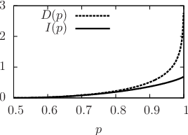
Hence, the contribution of the contact step to the dissipated work is greater than the contribution of separation step.

The situation is similar in the general case. Consider the setup depicted in section 3: $S$ is a thermodynamic system in contact with a heat bath at temperature $T$ and $p(x)$ its canonical distribution. The measurement device is also a thermodynamic system in contact with the heat bath and the energy of its micro-state either have some standard value $E_{M}^{0}(y)$ or are given by eq. (10), i.e. they are such that $p(y|x)$ is the canonical distribution for $M$ for a given value of $x$. Since the states of $M$ correspond to the possible measurement outcomes, it would make no sense that $y$ can take more values than $x$. However, formally, the following derivation is still valid in that case.

As in the previous section, we consider two different protocols for the measurement. Either the energy levels of $M$ are driven from the standard values $E_{M}^{0}(y)$ to the values corresponding to the measurement, $E_{M}(y|x)$ and then back to the standard values. Or the energies of $M$ initially have the values given by the previous measurement, i.e. $E_{M}(y|x^{\prime})$ with probability $p(x^{\prime})$, $x^{\prime}$ being the state of $S$ during the previous cycle, and are driven to the values corresponding to the actual measurement. We will see that for a suitable choice for $E_{M}^{0}(y)$, the two protocols give the same value for the work performed on $M$, as in the case of a two states system.

We set the values of $E_{M}^{0}(y)$ so that the marginal distribution of the measurement outcome $y$ is an equilibrium one:

$$E_{M}^{0}(y)=-kT\log p(y)+F_{M}^{0},$$

(20)

where $p(y)=\sum_{x}p(y|x)p(x)$ and $F_{M}^{0}$ is the free energy of $M$ in the standard state. If $S$ is in state $x$ when the measurement is carried on, then the average work performed on $M$ during the contact is given by:

$$W_{\rm cont}(x)=kT\sum_{y}p(y)\log\frac{p(y)}{p(y|x)}+\Delta F_{M}(x),$$

(21)

where $\Delta F_{M}(x)=F_{M}^{0}-F_{M}(x)$ is the change in free energy of $M$ during the process. Hence, on average over $x$, the work performed is

$$W_{\rm cont}=\sum_{x}p(x)W_{\rm cont}(x).$$

(22)

The work performed during the separation, conditioned on $x$ is given by

$$W_{\rm sep}(x)=kT\sum_{y}p(y|x)\log\frac{p(y|x)}{p(y)}-\Delta F_{M}(x).$$

(23)

As in the previous section, the average over $x$ of this quantity is linked to the mutual information between $x$ and $y$:

$$W_{\rm sep}=\sum_{x}p(x)W_{\rm sep}(x)=kTI-\Delta F_{M},$$

(24)

where $\Delta F_{M}=\sum_{x}p(x)\Delta F_{M}(x)$ is the average change in free energy of $M$ and $I$ is the mutual information given by eq. (6). The total work performed is the sum of the two contributions. It can be rewritten in following form:

$$W_{\rm tot}=kT\sum_{x,y}\left(p(x,y)-p(x)p(y)\right)\log p(y|x).$$

(25)

Let us now consider the second protocol. The measurement device is left untouched after the previous measurement and is thus in equilibrium with its energies set to $E_{M}(y|x^{\prime})$ for a certain $x^{\prime}$ appearing with probability $p(x^{\prime})$. Here, $x^{\prime}$ is the state the system $S$ was during the previous measurement. After the contact, the energies of $M$ are set to $E_{M}(y|x)$, where $x$ is the current state of $S$, appearing with probability $p(x)$ (independently of $x^{\prime}$). Given $x^{\prime}$ and $x$, the average work performed on $M$ is:

$$W^{\prime}(x^{\prime},x)=kT\sum_{y}p(y|x^{\prime})\log\frac{p(y|x^{\prime})}{p(y|x)}+F_{M}(x)-F_{M}(x^{\prime}).$$

(26)

On average over $x^{\prime}$ and $x$, we obtain following expression:

	$\displaystyle W^{\prime}$	$\displaystyle=$	$\displaystyle\sum_{x^{\prime},x}p(x^{\prime})p(x)W(x^{\prime},x)$		(27)
		$\displaystyle=$	$\displaystyle kT\sum_{x^{\prime},x,y}p(x^{\prime})p(x)p(y|x^{\prime})\log\frac{p(y|x^{\prime})}{p(y|x)}.$

Using the fact that $p(y)=\sum_{x^{\prime}}p(y|x^{\prime})p(x^{\prime})$, one can bring the above expression to the same form as eq. (25):

$$W^{\prime}=kT\sum_{x,y}\left(p(x,y)-p(x)p(y)\right)\log p(y|x)=W_{\rm tot}.$$

(28)

This extends the result obtained in the previous section for a two states system. It means that switching $M$ from a random state to another, or switching it from the standard state to a random state and then back to the standard state involves the same quantity of work on average.

In its original formulation, Landauer’s principle states that erasing one bit of information is necessarily accompanied by the dissipation of at least $kT\log 2$ of work [12]. Bennett used Landauer’s principle to propose a solution to Szilard’s paradox [13]. Let us briefly sketch the argument behind Landauer’s principle. Consider a one particle gas in a closed container in contact with a heat bath. The volume is divided in two by a removable partition. If the particle is in the left half of the container, it encodes one value, say “0” and if it is in the right half of the container, it encodes the other value, “1” in this case. Erasing the information contained in the memory means bringing the memory to a standard state, say the state “0”, without knowing the value that is encoded. Such a protocol need to bring both states “0” and “1” to “0”. An obvious way to proceed is to remove the partition and then compress the gas in the left half of the container. Such a process dissipates at least $kT\log 2$. The dissipation occurs during the free expansion of the gas right after the removal of the partition: the volume of the gas is doubled, i.e. its entropy is increased by $k\log 2$ and no heat is exchanged with the heat bath meaning that the entropy of the latter stays constant during this process. Compressing the gas in the left half of the container needs $kT\log 2$ of work which is then transferred to the heat bath in form of heat, thereby increasing its entropy by $k\log 2$. This result was extended to general memories, see e.g. [15].

If the bit was used to store the result of the measurement of the state of a two levels system, as in section 3, then the work needed to erase the bit surely compensates the maximum work that can be extracted with help of the measurement because $I(p)\leq\log 2$ with equality if and only if $p=1$ (or $p=0$), i.e. when there are no measurement errors. In [13], Bennett argues that the measurement can be performed reversibly. By this, he means that as long as we know in which state the memory is (say in the state encoding “0”, the standard state), we can reversibly drive it to “0” or to “1” according to the result of the measurement. We will call this process “recording of the information” rather than “ measurement”. However, this argument implies that the system $S$ does not evolve during the recording, so that the information is still useful when the process of recording is finished. This is not the case in general. Consider for instance the (imperfect) measurement of the position of a Brownian particle as presented in [3]: once one has measured the position of the particle, one should immediately perform a process depending on the measured position in order to convert all of the information into heat. In fact, the particle does not stop moving after the measurement. So if one takes an infinite time to reversibly record the information before using it, then once it will be recorded it will bring nothing anymore because the system will have relaxed back to equilibrium.

In our framework, the information about the result of the measurement is stored in a way similar to the situation considered in Landauer’s principle: the measurement device is in a probabilistic superposition of macroscopic states, on per value of $x$ and appearing with probability $p(x)$. However, there are two important differences. We do not only consider dissipation during the erasure step but also during the measurement itself. As argued above, reversible recording of the information implies that the fluctuation about which the information is recorded is “frozen”. If instead the system is still in contact with the heat bath and continues to evolve, then the driving of the measurement device needs to be fast. However, the main reason for the instantaneous changes in the energies of $M$ is that it should be directly driven by $S$: either the energies have a value that directly depends on $x$ or not. But we consider no in between. In our opinion, this is what makes the difference between “measurement” and “recording”. We consider “recording” to be the following process: we know the outcome of some measurement and we want to record it to some memory device. This can be done infinitely slowly and hence with an arbitrarily small dissipation. On the other hand, a “measurement” device is directly driven by the information which is measured, i.e. we do not have a direct control on it. What then makes the information utilizable is the fact that $M$ relaxes instantly. If $M$ is not fully relaxed, then the information obtained is less, but the work performed is the same.

Finally, let us remark that Landauer’s erasure step is analogous to our “separation” step. During this step, the measurement device is brought from a mixture of macro-states to the standard state similarly to Landauer’s bit, which is brought from a statistical mixture of “0” and “1” to the standard state “0”. And in fact, the work dissipated during this process is $kTI$, i.e. it exactly compensates the work extracted from the heat bath using the information $I$. One big difference however, is the presence of measurement errors. As already mentioned, in the situation considered here, unlike in the classical situation usually involved in Landauer’s principle, the different $p(y|x)$ may overlap for different values of $x$. Sagawa and Ueda extended Landauer’s principle to the situation with measurement errors [15]. But in their framework, the measurement errors consist of an erroneous recording of the information and the different macro-states of the memory encoding the different measurement outcome are still perfectly distinguishable.

We have presented a very simple model for a measurement device and a protocol for the measurement of thermal fluctuations. The basic considerations motivating this model are the following: the measurement device should be a physical system and should obey the laws of thermodynamics and its state should depend on the value which is measured. In particular, the measurement errors should at least include thermal fluctuations. In that respect, the model presented here is minimal: the measurement errors are only due to thermal fluctuations. We showed that under these assumptions, the measurement process itself already leads to dissipation of work in addition to the dissipation due to Landauer’s erasure principle.

We also showed that the work performed on the measurement device is the same, whether the measurement device is intialized in and eventually brought back to a standard state, or is simply left as it is at the end of the measurement process.

References

- [1] L. Szilard, Zeitschrift für Physik 53, 840 (1929).
- [2] S. Toyabe, T. Sagawa, M. Ueda, E. Muneyuki, and M. Sano, Nature Physics 6, 988 (2010), arXiv:1009.5287.
- [3] D. Abreu and U. Seifert, Euro. Phys. Lett. 94, 10001 (2011), arXiv:1102.3826.
- [4] H. H. Hasegawa, J. Ishikawa, K. Takara, and D. J. Driebe, Phys. Lett. A 374, 1001 (2010), arXiv:0907.1569.
- [5] K. Takara, H. H. Hasegawa, and D. J. Driebe, Phys. Lett. A 375, 88 (2010).
- [6] M. Esposito and C. Van den Broeck, Eur. Phys. Lett. 95, 40004 (2011), arXiv:1104.5165.
- [7] T. Sagawa and M. Ueda, Phys. Rev. Lett. 100, 080403 (2008), arXiv:0710.0956.
- [8] T. Sagawa and M. Ueda, Phys. Rev. Lett. 104, 090602 (2010), arXiv:0907.4914.
- [9] T. Sagawa and M. Ueda, Nonequilibrium thermodynamics of feedback control, arXiv:1105:3262, 2011.
- [10] J. M. Horowitz and S. Vaikuntanathan, Phys. Rev. E 82, 061120 (2010), arXiv:1011.4273.
- [11] M. Ponmurugan, Phys. Rev. E 82, 031129 (2010), arXiv:1004.4311.
- [12] R. Landauer, IBM J. Res. Dev. 5, 183 (1961).
- [13] C. H. Bennett, Int. J. Theor. Phys. 21, 905 (1982).
- [14] P. N. Fahn, Found. of Phys. 26, 71 (1996).
- [15] T. Sagawa and M. Ueda, Phys. Rev. Lett. 102, 250602 (2009), arXiv:0809.4098.
- [16] T. M. Cover and J. A. Thomas, Elements of Information Theory, Wiley-Intersciences, second edition, 2006.
- [17] J. Ladyman, S. Presnell, and A. J. Short, Studies in History and Philosophy of Modern Physics 39, 315 (2008).
- [18] J. M. Horowitz and J. M. R. Parrondo, Eur. Phys. Lett. 95, 10005 (2011), arXiv:1104.0332.
- [19] R. Kawai, J. M. R. Parrondo, and C. Van den Broeck, Phys. Rev. Lett. 98, 080602 (2007), arXiv:0707.2996.
- [20] A. Gomez-Marin, J. M. R. Parrondo, and C. Van den Broeck, Euro. Phys. Lett. 82, 50002 (2008), arXiv:0807.1027.