The Dark Matter Density Profile of the Fornax DwarfNote: Accepted to ApJ: 29 November 2011
Abstract
We construct axisymmetric Schwarzschild models to measure the mass profile of the local group dwarf galaxy Fornax. These models require no assumptions to be made about the orbital anisotropy of the stars, as is the case for commonly used Jeans models. We test a variety of parameterizations of dark matter density profiles and find cored models with uniform density fit significantly better than the cuspy halos predicted by cold dark matter simulations. We also construct models with an intermediate-mass black hole, but are unable to make a detection. We place a - upper limit on the mass of a potential intermediate-mass black hole at .
Subject headings
dark matter—galaxies: dwarf—galaxies: individual (Fornax)—galaxies: kinematics and dynamics—Local GroupI. Introduction
Low-mass galaxies provide a unique testing ground for predictions of the cold dark matter (CDM) paradigm for structure formation, since they generally have a lower fraction of baryons than massive galaxies. These galaxies allow for a more direct measurement of the underlying dark matter potential, as the complicated effects of baryons on the dark matter are less pronounced. A particularly testable prediction of CDM is that all galaxies share a universal dark matter density profile, characterized by a cuspy inner power law where (Navarro et al. 32, hereafter 32). Many authors have investigated low-mass spirals and found, in contrast to the predictions of CDM, dark matter density profiles with a flat inner core of slope [9, 34, 13, 7, 40]. This has launched the debate known as the core/cusp controversy.
A number of other studies have investigated the mass content of dwarf spheroidal galaxies (dSphs). Gilmore et al. [22] give a comprehensive review of recent attempts to constrain the inner slope of their dark matter profiles with Jeans modeling (Jeans 26; Binney & Tremaine 6, chapter 4). When significant, cored profiles are preferred for all dSphs modeled (Gilmore et al. 22, and references therein).
These results, however, are subject to a major caveat of Jeans modeling; it is complicated by the effect of stellar velocity anisotropy. Models fit to the line-of-sight component of the velocity dispersion, but anisotropy can severely affect the modeling of enclosed mass. Therefore, additional assumptions must be made. The studies presented in Gilmore et al. [22] assume spherical symmetry and isotropy. Evans et al. [16] show that a weakness of Jeans modeling is that given these assumptions combined with the cored light profiles observed in dSphs, the Jeans equations do not allow solutions with anything other than a cored dark matter profile.
Walker et al. [56] construct more sophisticated models and attempt to parameterize and fit for the anisotropy. As a result, preference for cored profiles becomes model-dependent. They therefore are unable to put significant constraints on the slope of the dark matter profile. This highlights the main problem with Jeans modeling—it is highly dependent on the assumptions made.
Distribution function models are more general than Jeans models, and progress has been made applying them to a number of dSph systems [28, 59, 2]. Nevertheless these models still make strong assumptions such as spherical symmetry or isotropy, and models that do fit for anisotropy do so without using the information about the stellar orbits contained in the line-of-sight velocity distributions (LOSVDs).
We employ a fundamentally different modeling technique, known as Schwarzschild modeling, that allows us to use this information to self-consistently calculate both the enclosed mass and orbital anisotropy. Schwarzschild modeling is a mature industry, but one that has seldom been applied to the study of dSph galaxies (see Valluri et al. 47).
In addition to being well-suited for measuring dark matter profiles, Schwarzschild modeling has often been used to search for black holes at the centers of galaxies. Another unresolved issue relevant to the study of dSphs is whether they host an intermediate-mass black hole (IMBH). In a hierarchical merging scenario, smaller galaxies are thought to be the building blocks of larger galaxies. It is thought that all massive galaxies host a supermassive black hole (SMBH) at their center, therefore it is logical to believe that their building blocks host smaller IMBHs. Evidence for these IMBHs is scarce, however, and dynamical detections are even scarcer. The closest and lowest mass example of a dynamical measurement is an upper limit on the local group dSph NGC 205 of [47]. Black holes in this mass range can provide constraints on theories of black hole growth and formation. The two most prominent competing theories of nuclear black hole formation are direct collapse of primordial gas [46, 14, 4] or accretion onto and mergers of seed black holes resulting from the collapse of the first stars [52].
In this paper we present axisymmetric, three-integral Schwarzschild models in an effort to determine the inner slope of the dark matter density profile as well as the orbit structure of the Fornax dSph. We also investigate the possibility of a central IMBH. We assume a distance of 135 kpc to Fornax [5].
II. Data
To construct dynamical models, we require a stellar light profile as well as stellar kinematics in the form of LOSVDs. We use published data for both the photometry and kinematics, and describe the steps taken to convert this data into useful input for our models.

II.1. Stellar Density
To determine the stellar density, we use a number density profile from Coleman et al. [11] extending to . We linearly extrapolate the profile out to —a physical radius of 3.9 kpc at our assumed distance. We also extrapolate the profile inwards at constant density from to .
To convert to a more familiar surface brightness profile we apply an arbitrary zero-point shift in log space, adjusting this number so that the integrated profile returns a luminosity consistent with the value listed in Mateo [30]. Adopting an ellipticity of [30], we deproject under the assumption that surfaces of constant luminosity are coaxial spheroids [19], and for an assumed inclination of .
II.2. Stellar Kinematics
We derive LOSVDs from individual stellar velocities published in Walker et al. [54]. The data contain heliocentric radial velocities and uncertainties with a membership probability for 2,633 Fornax stars. Most of these are single-epoch observations, however some are multi-epoch. Stars that have more than one observation are averaged, weighted by their uncertainties. After making a cut in membership probability at 90%, we are left with 2,244 stars. Although a significant number of stars observed may be in binary or multiple systems, simulations have shown that such systems are unlikely to affect measured dispersions [24, 33, 30].
We adopt a position angle [55]. We assume symmetry with respect to both the major and minor axes and fold the data along each axis. To preserve any possible rotation, we switch the sign of the velocity whenever a star is flipped about the minor axis.

The transverse motion of Fornax contributes a non-negligible line-of-sight velocity to stars, particularly those at large galactocentric radius. Using the equations in Appendix A of Walker et al. [53], we correct for this effect. We adopt values for the proper motion of [35] and assume the heliocentric radial velocity of Fornax is [36].
We divide our meridional grid into 20 radial bins, equally spaced in approximately from 1″to 5000″. There are 5 angular bins spaced equally in sin over 90∘ from the major to the minor axis [20, 41]. From the positions of the folded stellar velocity data, we determine the best binning scheme so that each grid cell contains at least 25 stars from which to recover the LOSVD. Our first bin with enough stars to meet this criterion is centered at 47″, and the last bin is centered at 2500″. We therefore have two-dimensional kinematics coverage over the radial range 47″-2500″(30pc - 1.6 kpc). At small radii the number density of stars with velocity measurements is low, thus our central LOSVDs have higher uncertainty compared to those at larger radii.
| DM Profile | c | (kpc) | () | () | |||
|---|---|---|---|---|---|---|---|
| NFW | 239.8 | — | — | 3124 | |||
| Log | 162.6 | — | — | — | 4319 | ||
| Log | 162.6 | — | — | 3423 |
Note. — Best-fit parameters for NFW, and cored logarithmic dark matter halos. is un-reduced, the number of degrees of freedom are the same for each model. Model parameters and - uncertainties are quoted. lists the number of models run for the corresponding parameterization.
Within each grid cell, we calculate the LOSVD from discrete stellar velocities by using an adaptive kernel density estimate adapted from Silverman [39] and explained in Gebhardt et al. [19]. We estimate the uncertainties in the LOSVDs through bootstrap resamplings of the data [19, 18]. The bootstrap generates a new sample from the data itself by randomly picking data points, where is the total number of stars in a given bin, allowing the same point to be chosen more than once. We then estimate the LOSVD from that realization and repeat the procedure times. The confidence band on the LOSVDs corresponds to the range of the realizations. We compare the velocity dispersion as measured by the LOSVDs with the biweight scale (i.e., a robust estimate of the standard deviation, see Beers et al. 3) of the individual velocities and note good agreement.
Figure 1 plots the LOSVDs of four bins. Rather than parameterizing these LOSVDs with Gauss-Hermite moments, our models instead fit directly to the LOSVDs to constrain the kinematics of the galaxy. However, we do fit Gauss-Hermite moments for plotting purposes only. These data are presented in Figure 2 for stars that have been grouped into bins near the major axis (blue) and minor axis (red). Near the center of the galaxy the density of stars with kinematics is sparse, so we therefore group stars into annular bins covering all angles (green). We estimate the - uncertainties of the Gauss-Hermite moments by fitting to each of the 300 realizations calculated during the bootstrap discussed above. The error bars plotted contain 68% of the 300 realizations.
III. Dynamical Models
The modeling code we use is described in detail in Gebhardt et al. [21],Thomas et al. [44], Thomas et al. [43], and Siopis et al. [41] and is based on the technique of orbit superposition [38]. Similar axisymmetric codes are described in Rix et al. [37], van der Marel et al. [50], Cretton et al. [12], Valluri et al. [48] while van den Bosch et al. [49] present a fully triaxial Schwarzschild code. Our code begins by choosing a trial potential that is a combination of the stellar density, dark matter density, and possibly a central black hole. We then launch orbits carefully chosen to uniformly sample the isolating integrals of motion. In an axisymmetric potential, orbits are restricted by three isolating integrals of motion, , , and the non-classical “third integral” . As it is not possible to calculate a priori, we use a carefully designed scheme to systematically sample for each pair of and [44, 41]. Orbits are integrated for many dynamical times, and each orbit is given a weight . We find the combination of that best reproduces the observed LOSVDs and light profile via a minimization subject to the constraint of maximum entropy [41].
We run models by varying 3 parameters—the stellar and two parameters specifying the dark matter density profile. Some models are also run with a central black hole whose mass is varied in addition to the other 3 model parameters. Each model is assigned a value of and we identify the best-fitting model as that with the lowest . We determine the confidence range on parameters by identifying the portion of their marginalized curves that lie within of the overall minimum.
III.1. Model Assumptions
Our trial potential is determined by solving Poisson’s equation for an assumed trial density distribution. On our two-dimensional polar grid, this takes the form:
| (1) |
where is the stellar mass-to-light ratio, assumed constant with radius, and is the unprojected luminosity density. The assumed dark matter profile is discussed below. For simplicity, we assume Fornax is edge-on in all our models.
III.2. Dark Matter Density Profiles
We parameterize the dark matter halo density with a number of spherical density profiles. We use NFW halos:
| (2) |
where
and is the present critical density for a closed universe. The two parameters we fit for are the concentration and scale radius . We also use halos derived from the logarithmic potential:
| (3) |
These models feature a flat central core of density for and an profile for . We fit for and , the asymptotic circular speed at and core radius respectively. We run over 10,000 models with only three distinct parameterizations: NFW halos, and logarithmic models with and without an IMBH.
IV. Results
We find significant evidence for cored logarithmic dark matter density profiles. These models are preferred at the level when compared to models with an NFW halo, a highly significant result. Perhaps more convincingly, the values for the concentration preferred by our models are around . Only relatively recently formed structures like galaxy clusters are expected to have concentrations this low [32].
Table 1 summarizes the results of our models, while Figures 1 and 2 illustrate the preference for cored models over models with an NFW halo in fitting to the kinematics. We stress again that LOSVDs like those plotted in Figure 1 are the kinematic constraint, and not the Gauss-Hermite moments of Figure 2.
While we fit for and in the cored models, these parameters are strongly degenerate. Our model grid extends to kpc, thus any model with kpc has a uniform density over the entire range of our model. Furthermore, we have no velocity information from stars past and therefore cannot constrain the kinematics in the outer parts of the galaxy. Thus, for models with , is now the only parameter that differentiates between models. As is dependent on both and , the latter two parameters are completely degenerate.
Figure 3 illustrates this effect. Plotted are the curves for each model parameter. Lines of the same color indicate a common parameterization of the mass profile (e.g. cored + IMBH). While the for both and asymptotes to large values, is tightly constrained. Note that the behavior of for logarithmic profiles with an IMBH (green line) is a result of incomplete parameter sampling. With a more densely-sampled parameter space, the curve for for cored models with an IMBH would likely asymptote to large in a similar fashion as models without an IMBH (red curve).
The addition of a central black hole to the mass profile does not make a noticeable difference to the overall for most values of . We therefore place a - upper limit on .
We plot the mass profile for our best-fit model in Figure 4 (solid black line with surrounding confidence region). This is a cored logarithmic dark matter profile without a central black hole. The mass profile of our best-fit dark halo is plotted as the dashed line, and the stellar mass profile is plotted in red. The contribution of dark matter to the total mass increases with radius as the local dynamical mass-to-light ratio rises from approximately to greater than 100 in the outermost bin of our model.
IV.1. Orbit Structure
We construct a distribution function for the galaxy from the set of orbital weights resulting from the minimization of our best-fit model. To explore the orbit structure, we determine the internal (unprojected) moments of the distribution function in spherical coordinates. Streaming motions in the and directions are assumed to be zero. In this coordinate system, cross-terms of the velocity dispersion tensor are zero.

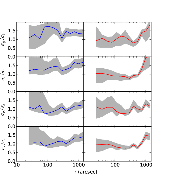
Figure 5 plots the anisotropy in the diagonal components of the dispersion tensor. While some panels show an average value near unity, there are regions in every panel where the ratio plotted is different from one. Additionally, we define the tangential velocity dispersion where is the second moment , and is the mean rotation velocity. With this definition, we plot the ratio in the bottom panels of Figure 5 to investigate whether orbits are radially or tangentially biased. From these plots it is clear that the common assumptions of Jeans modeling—constant or zero anisotropy—are unrealistic. We find that at most radii in the galaxy, orbits are radially biased. The uncertainty in the anisotropy is largest at small radii, as evidenced by the size of the 68% confidence regions in Figure 5. This is likely due to the sparsity of kinematics in the inner part of the galaxy (there are limits to how closely target fibers can be spaced in multi-fiber spectroscopy).
In a recent paper, Kazantzidis et al. [27] simulated the effects of tidal stirring on a number of dSph progenitors around a Milky Way sized halo. They found radial anisotropy in all of the final remnants, and our models are consistent with these findings.
V. Discussion
V.1. Cores and Cusps
Our analysis shows that for the Fornax dwarf an NFW dark matter halo with inner slope is rejected with high confidence. We have kinematics from pc- kpc, and over this range the models prefer an uniform density core with . We do not attempt to fit for models with an intermediate value of the slope . Further investigation is necessary before we can conclude that the best fitting dark matter profile is the logarithmic model. The steep cusp of the NFW profile is, however, robustly ruled out.
The models, in general, seem to prefer less mass in the areas over which we have kinematic constraints. In NFW models, the concentration sets the normalization (or y-intercept) of the density profile. Because cannot be lowered below an astrophysically reasonable limit, NFW models enclose more mass than cored models. This difference is reflected in the difference between cored and NFW models, as the kinematics are best fit by models with less mass. Figure 2 hints at this as the best fit NFW model (dashed line) typically has higher values for than either the data or best-fitting cored model (solid line).
Several groups have approached the core/cusp issue in dSphs by taking advantage of the fact that some dSphs host multiple populations of tracer stars that are chemically and dynamically distinct. By fitting models to each component, the underlying dark matter profile can be modeled more accurately. Amorisco & Evans [1] fit two-component distribution function models to Sculptor, while Walker & Peñarrubia [57] apply a convenient mass estimator (discussed below) to each stellar component in Sculptor and Fornax. It is believed that this mass estimator is unaffected by orbital anisotropy, thus their method yields a robust determination of the dynamical mass at two locations in the galaxy—allowing for the slope of the dark matter profile to be measured. Each of these studies finds models with a cored dark matter halo preferable to the predicted cuspy NFW profile.
It must be noted, however, that we are not observing the pristine initial dark matter distribution in this galaxy. Rather, it has likely been modified by complex baryonic processes over the lifetime of the galaxy. These processes may include: adiabatic compression [8], halo rebounding following baryonic mass loss from supernovae [31], or possibly dynamical friction acting on clumps of baryons (El-Zant et al. 15; but see also Jardel & Sellwood 25). Although we chose this galaxy because these effects were likely to be small, they are nevertheless not well understood and our result must be taken in that context.
V.2. Central IMBH
We are unable to place a significant constraint on the mass of a central IMBH. Figure 3 (upper right) shows the marginalized curve against IMBH mass for cored dark matter density profiles. The curve asymptotes to low values of IMBH, thus we are only capable of placing an upper limit on the mass of any potential IMBH. Furthermore, our best-fit cored model with and without an IMBH have the same . We therefore impose a - upper limit on . It is unfortunate that we are not able to place a lower limit on because measurements of black holes in the range place direct constraints on SMBH formation mechanisms (van Wassenhove et al. 2010 ). Our models, however, do robustly rule out a black hole of larger mass.
In massive galaxies it is thought that the radius of influence, must be resolved in order to detect and precisely measure a black hole [21, 29, 17, 23]. Using our upper limit on we can calculate the maximum radius of influence of a potential black hole. Estimating the central velocity dispersion at gives an upper limit for pc. Our kinematics start at pc, so it is not surprising that the minimum black hole mass we were able to detect has close to pc. To detect smaller black holes, we require kinematics of stars closer to the center of the galaxy.
We are able to detect the dynamical influence of a black hole with a similar mass as Valluri et al. [47] detect in NGC 205, however with kinematics of much lower resolution. Our innermost model bin is centered around whereas they use high-resolution kinematics from the Hubble Space Telescope to resolve spatial scales less than . The advantage we have is that the central velocity dispersion is much smaller in Fornax, which makes larger for fixed . NGC 205 is also more than five times as distant as Fornax.
V.3. Mass Estimators
Several authors have come up with convenient estimators of total mass within a given radius for local group dSphs. Strigari et al. [42] use the mass enclosed within pc while Walker et al. [56] and Wolf et al. [58] find a similar expression for the mass contained within the projected and un-projected half-light radii, respectively. These estimators bear striking resemblance to a result obtained by Cappellari et al. [10] derived from integral field kinematics of massive elliptical galaxies, and they all hint at an easy way to determine dynamical masses without expensive modeling. They are believed to be insensitive to velocity anisotropy based on the derivation in Wolf et al. [58], and we compare their estimates to our models as a check on this.
For the mass contained within pc we measure , roughly a factor of three smaller than Strigari et al. [42] who measure using Jeans models with parameterized anisotropy.
The Cappellari et al. [10], Walker et al. [56], and Wolf et al. [58] mass estimators are all of the form:
| (4) |
where is the radius at which the estimator is valid. For Cappellari et al. [10] and Walker et al. [56] (the projected half-light radius), while for Wolf et al. [58] (the un-projected half-light radius). Other than the projected/un-projected difference, each estimator differes only by the value of the constant . In order to more fairly compare between these estimators and our models, we use the values for the luminosity-weighted line-of-sight velocity dispersion projected half-light radius , and un-projected half-light radius that we calculate from the data used in our models.
Our best-fitting model has and . With each group’s value for and our kinematics, the mass estimates are: [56], [58], and [10]. Our model is broadly consistent with both the Walker et al. [56] and Wolf et al. [58] estimators.
The evidence that mass estimators are anisotropy-independent comes largely from comparison to spherical Jeans models (except Cappellari et al. 10). The weakness of these models is that the anisotropy must be parameterized and is restricted to be a function of radius only. Our models are not subject to these constraints since the anisotropy is calculated non-parametrically and is free to vary with position angle. We suggest that the best way to prove the accuracy of mass estimators is to compare with models that can self-consistently calculate both mass and anisotropy for realistic potentials.
For bright elliptical galaxies, Cappellari et al. [10] and Thomas et al. [45] have done just that. In these cases, the mass estimates are checked against masses derived from axisymmetric Schwarzschild modeling and good agreement is found. Ours is the first study to perform a similar test with dSphs, and there is no reason to assume that success with bright ellipticals guarantees accuracy in the dSph regime. The results from our comparison above are nevertheless reassuring.
V.4. Tidal Effects
The principle of orbit superposition, and hence our entire modeling procedure, relies on the assumption that the galaxy is bound and in a steady state. The amount of tidal stripping in Fornax due to the effect of its orbit through the Milky Way’s halo is not well-known. For reasonable values of Fornax total mass , Milky Way mass , and Galactocentric radius , the tidal radius of Fornax is . This estimate of is sufficiently larger than our model grid that we would not expect tidal effects to be important over the radial range of our models. If Fornax is on an eccentric orbit about the Milky Way, however, the above equation for is not valid and estimation of the tidal radius is not as straightforward. Fortunately, studies investigating its transverse motion suggest the orbit of Fornax is roughly circular [35, 53].
References
- [1] Amorisco, N. C., & Evans, N. W. 2011a, MNRAS, 1606
- [2] —. 2011b, MNRAS, 411, 2118
- [3] Beers, T. C., Flynn, K., & Gebhardt, K. 1990, AJ, 100, 32
- [4] Begelman, M. C., Volonteri, M., & Rees, M. J. 2006, MNRAS, 370, 289
- [5] Bersier, D. 2000, ApJL, 543, L23
- [6] Binney, J., & Tremaine, S. 1987, Galactic dynamics, ed. Binney, J. & Tremaine, S.
- [7] Blais-Ouellette, S., Amram, P., & Carignan, C. 2001, AJ, 121, 1952
- [8] Blumenthal, G. R., Faber, S. M., Flores, R., & Primack, J. R. 1986, ApJ, 301, 27
- [9] Burkert, A. 1995, ApJL, 447, L25+
- [10] Cappellari, M., et al. 2006, MNRAS, 366, 1126
- [11] Coleman, M. G., Da Costa, G. S., Bland-Hawthorn, J., & Freeman, K. C. 2005, AJ, 129, 1443
- [12] Cretton, N., de Zeeuw, P. T., van der Marel, R. P., & Rix, H. 1999, ApJS, 124, 383
- [13] de Blok, W. J. G., McGaugh, S. S., Bosma, A., & Rubin, V. C. 2001, ApJL, 552, L23
- [14] Eisenstein, D. J., & Loeb, A. 1995, ApJ, 443, 11
- [15] El-Zant, A., Shlosman, I., & Hoffman, Y. 2001, ApJ, 560, 636
- [16] Evans, N. W., An, J., & Walker, M. G. 2009, MNRAS, 393, L50
- [17] Ferrarese, L., & Ford, H. 2005, Space Science Reviews, 116, 523
- [18] Gebhardt, K., & Thomas, J. 2009, ApJ, 700, 1690
- [19] Gebhardt, K., et al. 1996, AJ, 112, 105
- [20] —. 2000, ApJL, 539, L13
- [21] —. 2003, ApJ, 583, 92
- [22] Gilmore, G., Wilkinson, M. I., Wyse, R. F. G., Kleyna, J. T., Koch, A., Evans, N. W., & Grebel, E. K. 2007, ApJ, 663, 948
- [23] Gültekin, K., et al. 2009, ApJ, 698, 198
- [24] Hargreaves, J. C., Gilmore, G., & Annan, J. D. 1996, MNRAS, 279, 108
- [25] Jardel, J. R., & Sellwood, J. A. 2009, ApJ, 691, 1300
- [26] Jeans, J. H. 1919, Royal Society of London Philosophical Transactions Series A, 218, 157
- [27] Kazantzidis, S., Łokas, E. L., Callegari, S., Mayer, L., & Moustakas, L. A. 2011, ApJ, 726, 98
- [28] Kleyna, J., Wilkinson, M. I., Evans, N. W., Gilmore, G., & Frayn, C. 2002, MNRAS, 330, 792
- [29] Kormendy, J. 2004, in Coevolution of Black Holes and Galaxies, ed. L. C. Ho, 1–+
- [30] Mateo, M. L. 1998, ARA&A, 36, 435
- [31] Navarro, J. F., Eke, V. R., & Frenk, C. S. 1996a, MNRAS, 283, L72
- [32] Navarro, J. F., Frenk, C. S., & White, S. D. M. 1996b, ApJ, 462, 563
- [33] Olszewski, E. W., Pryor, C., & Armandroff, T. E. 1996, AJ, 111, 750
- [34] Persic, M., Salucci, P., & Stel, F. 1996, MNRAS, 281, 27
- [35] Piatek, S., Pryor, C., Bristow, P., Olszewski, E. W., Harris, H. C., Mateo, M., Minniti, D., & Tinney, C. G. 2007, AJ, 133, 818
- [36] Piatek, S., et al. 2002, AJ, 124, 3198
- [37] Rix, H., de Zeeuw, P. T., Cretton, N., van der Marel, R. P., & Carollo, C. M. 1997, ApJ, 488, 702
- [38] Schwarzschild, M. 1979, ApJ, 232, 236
- [39] Silverman, B. W. 1986, Density estimation for statistics and data analysis, ed. Silverman, B. W.
- [40] Simon, J. D., Bolatto, A. D., Leroy, A., Blitz, L., & Gates, E. L. 2005, ApJ, 621, 757
- [41] Siopis, C., et al. 2009, ApJ, 693, 946
- [42] Strigari, L. E., Bullock, J. S., Kaplinghat, M., Simon, J. D., Geha, M., Willman, B., & Walker, M. G. 2008, Nature, 454, 1096
- [43] Thomas, J., Saglia, R. P., Bender, R., Thomas, D., Gebhardt, K., Magorrian, J., Corsini, E. M., & Wegner, G. 2005, MNRAS, 360, 1355
- [44] Thomas, J., Saglia, R. P., Bender, R., Thomas, D., Gebhardt, K., Magorrian, J., & Richstone, D. 2004, MNRAS, 353, 391
- [45] Thomas, J., et al. 2011, MNRAS, 415, 545
- [46] Umemura, M., Loeb, A., & Turner, E. L. 1993, ApJ, 419, 459
- [47] Valluri, M., Ferrarese, L., Merritt, D., & Joseph, C. L. 2005, ApJ, 628, 137
- [48] Valluri, M., Merritt, D., & Emsellem, E. 2004, ApJ, 602, 66
- [49] van den Bosch, R. C. E., van de Ven, G., Verolme, E. K., Cappellari, M., & de Zeeuw, P. T. 2008, MNRAS, 385, 647
- [50] van der Marel, R. P., Cretton, N., de Zeeuw, P. T., & Rix, H. 1998, ApJ, 493, 613
- [51] van Wassenhove, S., Volonteri, M., Walker, M. G., et al. 2010, MNRAS, 408, 1139
- [52] Volonteri, M., & Perna, R. 2005, MNRAS, 358, 913
- [53] Walker, M. G., Mateo, M., & Olszewski, E. W. 2008, ApJL, 688, L75
- [54] —. 2009a, AJ, 137, 3100
- [55] Walker, M. G., Mateo, M., Olszewski, E. W., Bernstein, R., Wang, X., & Woodroofe, M. 2006, AJ, 131, 2114
- [56] Walker, M. G., Mateo, M., Olszewski, E. W., Peñarrubia, J., Wyn Evans, N., & Gilmore, G. 2009b, ApJ, 704, 1274
- [57] Walker, M. G., & Peñarrubia, J. 2011, ArXiv e-prints
- [58] Wolf, J., Martinez, G. D., Bullock, J. S., Kaplinghat, M., Geha, M., Muñoz, R. R., Simon, J. D., & Avedo, F. F. 2010, MNRAS, 406, 1220
- [59] Wu, X. 2007, ArXiv Astrophysics e-prints