跳到论文正文
W Papers独立论文阅读器 arXiv:1112.0311 论文正文 计算阅读时间 · 0%
引用这篇论文根据当前论文元数据生成,正式投稿前建议核对。


License: arXiv.org perpetual non-exclusive license
arXiv:1112.0311v2 [math.ST] 01 Dec 2012

Anisotropic Nonlocal Means Denoising

Journal: Applied and Computational Harmonic Analysis
Arian Maleki Email: arian.maleki@rice.edu URL: http://www.ece.rice.edu/˜mam15/ Corresponding author: Corresponding author    Manjari Narayan Email: manjari@rice.edu URL: http://www.ece.rice.edu/˜mn4/    Richard G. Baraniuk Email: richb@rice.edu URL: http://web.ece.rice.edu/richb/ Address: Dept. of Computer and Electrical Engineering, Rice University, MS-380
6100 Main Street, Houston, TX 77005, USA
Corresponding author: Principal corresponding author Note: Phone: +1 713.348.5132; Fax: +1 713.348.5685
Abstract

It has recently been proved that the popular nonlocal means (NLM) denoising algorithm does not optimally denoise images with sharp edges. Its weakness lies in the isotropic nature of the neighborhoods it uses to set its smoothing weights. In response, in this paper we introduce several theoretical and practical anisotropic nonlocal means (ANLM) algorithms and prove that they are near minimax optimal for edge-dominated images from the Horizon class. On real-world test images, an ANLM algorithm that adapts to the underlying image gradients outperforms NLM by a significant margin.

Keywords: 
Denoising, nonlocal means, minimax risk, anisotropy

1 Introduction

Image denoising is a fundamental primitive in image processing and computer vision. Denoising algorithms have evolved from the classical linear and median filters to more modern schemes like total variation denoising Rudin et al. [1992], wavelet thresholding Johnstone [2011], and bilateral filters Smith and Brady [1997], Yaroslavsky [1985], Tomasi and Manduchi [1998], Elad [2002].

A particularly successful denoising scheme is the nonlocal means (NLM) algorithm Buades et al. [2005], which estimates each pixel value as a weighted average of other, similar noisy pixels. However, instead of using spatial adjacency or noisy pixel value as the similarity measure to adjust the estimate weights, NLM uses a more reliable notion of similarity based on the resemblance of the pixels’ neighborhoods in high-dimensional space. This unique feature benefits NLM in two ways. First, it provides more accurate weight estimates. Second, it enables NLM to exploit the contribution of all pixels in the image. In concert, these features enable NLM to provide remarkable performance for a large class of image denoising problems.

Refer to caption
Figure 1: An example of a Horizon class image that features a smooth edge contour that separates the white region from the black region.

Nevertheless, in a recent paper, we have proved that NLM does not attain optimal performance on images with sharp edges from the so-called Horizon class (see Figure 1) Maleki et al. [2012a].11 1 Recently Arias-Castro et al. [2012] has extended our results to more complicated image//\penaltyedge models. Indeed, NLM’s theoretical performance is more or less equivalent to wavelet thresholding, which was shown to be suboptimal in Donoho [1999]. Empirical results have also confirmed the suboptimality of NLM in estimating sharp edges Duval et al. [2011], Salmon and Strozecki [2010], Deledalle et al. [2011], Dabov et al. [2008]. The core problem is that NLM (and wavelet thresholding) cannot exploit the smoothness of the edge contour that separates the white and black regions.

In this paper, we introduce and study a new denoising framework and prove that it is near-optimal for Horizon class images with sharp edges. Anisotropic nonlocal means (ANLM) outperforms NLM, wavelet thresholding, and more classical techniques by using anisotropic neighborhoods that are elongated along and matched to the local edge orientation. Figure 2 compares the neighborhoods used in ANLM with those used in NLM. Anisotropic neighborhoods enable ANLM to distinguish between similar and dissimilar pixels more accurately.

Refer to caption
Figure 2: Comparison of (left) the isotropic neighborhoods employed by Non Local Means (NLM) versus (right) anisotropic neighborhoods employed by Anisotropic NLM (ANLM).

We develop three different ANLM algorithms of increasing levels of practicality. Oracle Anisotropic Nonlocal Means (OANLM) assumes perfect knowledge of the local orientation of the edge contour and is used primarily for our theoretical optimality analysis. Discrete-angle Anisotropic Nonlocal Means (DANLM) optimizes the choice of the anisotropic neighborhood around each pixel in order to achieve near-optimal performance without any oracle information. Since it is more computationally demanding than NLM, we introduce an algorithmic simplification. Gradient based Anisotropic Nonlocal Means (GANLM) uses image gradient information to estimate the edge orientation; using simulations, we demonstrate that GANLM significantly outperforms NLM in practice on both Horizon class and real-world images.

Anisotropy is a fundamental feature of real-world images. Hence, many denoising algorithms have been proposed to exploit this feature Nagao and Matsuyama [1979], Takeda [2006], Takeda et al. [2007], Perona and Malik [1990], Candès and Donoho [1999], Candès and Donoho [1999], Willett and Nowak [2003], Willett and Nowak [2007], Kutyniok and Labate [2007], Do and Vetterli [2005], Pennec and Mallat [2005], Velisavljevic et al. [2006], Deledalle et al. [2011], Salmon and Strozecki [2010], Dabov et al. [2008]. We will review all these algorithms and their similarities and differences with ANLM in Section 5.

The paper is organized as follows. Section 2 explains the minimax framework we use to analyze the denoising algorithms and reviews the necessary background. Section 3 introduces the OANLM and DANLM algorithms and presents the main theorems. Section 4 addresses some of the practical ANLM issues by introducing GANLM and summarizes the results of a range of simulations using synthetic and real-world imagery. Section 5 reviews the related work in the literature. Section 6 discusses our current and potential future results. Section 7 contains the proofs of the main theorems.

2 Minimax analysis framework

In this section we introduce the minimax framework Johnstone [2011], Lehman and Casella [1998] and the Horizon class image model considered in this paper. Note that, in order to streamline the proofs, we take a continuous-variable analysis approach in this paper, in contrast to our approach in Maleki et al. [2012a]. The moral of the story is compatible with Maleki et al. [2012a], however.

2.1 Risk

We are interested in estimating an image described by the function f:[0,1]2→[0,1]f:[0,1]^{2}\rightarrow[0,1] (f∈L2​([0,1]2)f\in L^{2}([0,1]^{2})) from its noisy observation

d​Y​(t1,t2)=f⁡(t1,t2)​d​t1​d​t2+σ​d​W​(t1,t2).dY(t_{1},t_{2})=f(t_{1},t_{2})dt_{1}dt_{2}+\sigma dW(t_{1},t_{2}). (1)

Without loss of generality, we consider only square images. Here W⁡(t1,t2)W(t_{1},t_{2}) is the Wiener sheet,22 2 The Wiener sheet is the primitive of white noise. and σ\sigma is a constant that scales the noise. For a given function ff and a given estimator f^\hat{f}, define the risk as

R⁡(f,f^)=𝔼⁡(‖f−f^‖22),R(f,\hat{f})=\mathds{E}(\|f-\hat{f}\|_{2}^{2}),

where the expected value is over WW. The risk can be decomposed into bias squared and variance terms

R⁡(f,f^)=‖f−𝔼​f^‖22+𝔼​‖f^−𝔼​f^‖22.R(f,\hat{f})=\|f-\mathds{E}\hat{f}\|_{2}^{2}+\mathds{E}\|\hat{f}-\mathds{E}\hat{f}\|_{2}^{2}.

Let ff belong to a class of functions ℱ\mathcal{F}. The risk of the estimator f^\hat{f} on ℱ\mathcal{F} is defined as the risk of the least-favorable function, i.e.,

R⁡(ℱ,f^)=supf∈ℱR⁡(f,f^).R(\mathcal{F},\hat{f})=\sup_{f\in\mathcal{F}}R(f,\hat{f}).

The minimax risk over the class of functions ℱ\mathcal{F} is then defined as

R∗​(ℱ)=inff^supf∈ℱR⁡(f,f^).R^{*}(\mathcal{F})=\inf_{\hat{f}}\sup_{f\in\mathcal{F}}R(f,\hat{f}).

R∗​(ℱ)R^{*}(\mathcal{F}) is a lower bound for the performance of any estimator on ℱ\mathcal{F}.

In this paper, we are interested in the asymptotic setting as σ→0\sigma\rightarrow 0. For all the estimators we consider, R⁡(ℱ,f^)→0R(\mathcal{F},\hat{f})\rightarrow 0 as σ→0\sigma\rightarrow 0. Therefore, following Peyrè et al. [2007], Candès and Donoho [2002] we will consider the decay rate of the minimax risk as our measure of performance. For this purpose, we will use the following asymptotic notation.

Definition 1.

f⁡(σ)=O⁡(g⁡(σ))f(\sigma)=O(g(\sigma)) as σ→0\sigma\rightarrow 0, if and only if there exist σ0\sigma_{0} and cc such that for any σ<σ0\sigma<\sigma_{0}, |f⁡(σ)|≤c​|g⁡(σ)||f(\sigma)|\leq c|g(\sigma)|. Likewise, f⁡(σ)=Ω⁡(g⁡(σ))f(\sigma)=\Omega(g(\sigma)) as σ→0\sigma\rightarrow 0, if and only if there exist σ0\sigma_{0} and cc such that for any σ<σ0\sigma<\sigma_{0}, |f⁡(σ)|≥c​|g⁡(σ)||f(\sigma)|\geq c|g(\sigma)|. Finally, f⁡(σ)=Θ⁡(g⁡(σ))f(\sigma)=\Theta(g(\sigma)), if and only if f⁡(σ)=O⁡(g⁡(σ))f(\sigma)=O(g(\sigma)) and f⁡(σ)=Ω⁡(g⁡(σ))f(\sigma)=\Omega(g(\sigma)). We may interchangeably use f⁡(σ)≍g⁡(σ)f(\sigma)\asymp g(\sigma) for f⁡(σ)=Θ⁡(g⁡(σ))f(\sigma)=\Theta(g(\sigma)).

Definition 2.

f⁡(σ)=o⁡(g⁡(σ))f(\sigma)=o(g(\sigma)) if and only if limσ→0f⁡(σ)g⁡(σ)=0\lim_{\sigma\rightarrow 0}\frac{f(\sigma)}{g(\sigma)}=0.

2.2 Horizon edge model

In our analysis, we consider the Horizon model that contains piecewise constant images with sharp step edges lying along a smooth contour Donoho [1999], Peyrè et al. [2007], Korostelev and Tsybakov [1993] (our analysis extends easily to piecewise smooth edges). Let H​o¨​𝑙𝑑𝑒𝑟α​(C){\sl H\ddot{o}lder}^{\alpha}(C) be the class of Ho¨\rm\ddot{o}lder functions on ℝ\mathds{R}, defined in the following way: h∈H​o¨​𝑙𝑑𝑒𝑟α​(C)h\in{\sl H\ddot{o}lder}^{\alpha}(C) if and only if

|h(k)​(t1)−h(k)​(t1′)|≤C​|t1−t1′|α−k,|h^{(k)}(t_{1})-h^{(k)}(t^{\prime}_{1})|\leq C|t_{1}-t^{\prime}_{1}|^{\alpha-k},

where k=⌊α⌋k=\lfloor\alpha\rfloor. Consider a transformation that maps each one-dimensional edge contour function hh to a two-dimensional image fh:[0,1]2→[0,1]f_{h}:[0,1]^{2}\rightarrow[0,1] via

fh(t1,t2)=1{t2<h(t1)}.\displaystyle f_{h}(t_{1},t_{2})=\textbf{1}_{\{t_{2}<h(t_{1})\}}.

The Horizon class of images is then defined as

Hα​(C)={fh​(t1,t2):h∈H​o¨​𝑙𝑑𝑒𝑟α​(C)∩H​o¨​𝑙𝑑𝑒𝑟1​(1)},\displaystyle H^{\alpha}(C)=\{f_{h}(t_{1},t_{2}):h\in{\sl H\ddot{o}lder}^{\alpha}(C)\cap{\sl H\ddot{o}lder}^{1}(1)\}, (2)

where α\alpha is the smoothness of the edge contour. Figure 1 illustrates a sample function of this class. The following theorem characterizes the minimax rate of Hα​(C)H^{\alpha}(C) Donoho [1999], Peyrè et al. [2007], Korostelev and Tsybakov [1993].33 3 The models considered in Donoho [1999], Peyrè et al. [2007], Korostelev and Tsybakov [1993] are slightly different from the continuous framework of this paper. Therefore, for the sake of completeness we prove Theorem 1 in C.

Theorem 1.

Donoho [1999], Peyrè et al. [2007], Korostelev and Tsybakov [1993] For α≥1\alpha\geq 1, the minimax risk of the class Hα​(C)H^{\alpha}(C) is

R∗​(Hα​(C))=Θ⁡(σ2​αα+1).R^{*}(H^{\alpha}(C))=\Theta\!\left(\sigma^{\frac{2\alpha}{\alpha+1}}\right).

Achieving the minimax rate is a laudable goal that any well-respecting denoising algorithm should aspire to. In this paper, we will focus primarily on α=2\alpha=2 edge contours, for which the optimal minimax decay rate is σ4/3\sigma^{4/3}. However, it is straightforward to draw similar conclusions for the other values of α\alpha.

2.3 Image denoising algorithms

Minimax risk analysis of the classical denoising algorithms has revealed their suboptimal performance on images with sharp edges. Table 1 summarizes several of these algorithms and their minimax decay rates (up to a log factor).44 4 The analysis framework used in Arias-Castro and Donoho [2009] and Maleki et al. [2012a] is discrete rather than continuous. Therefore, for the sake of completeness we establish the results for the mean filter and NLM in A and B, respectively. The suboptimality of wavelet thresholding has led to the development of ridgelets Candès and Donoho [1999], curvelets Candès and Donoho [1999], wedgelets Donoho [1999], platelets Willett and Nowak [2003], shearlets Kutyniok and Labate [2007], contourlets Do and Vetterli [2005], bandelets Pennec and Mallat [2005], directionlets Velisavljevic et al. [2006] and other types of directional transforms. See Maleki et al. [2012b], Jacques et al. [2011] and the references therein for more information. In the framework of this paper, wedgelet denoising Donoho [1999] provably achieves the optimal minimax rate. However, it performs poorly on textures, which has limited its application in image processing.

Table 1: Minimax risk decay rates of several classical image denoising algorithms; recall that the according to Theorem 1, for α=2\alpha=2 the optimal minimax rate is σ4/3\sigma^{4/3}.
Algorithm Minimax Rate
Mean filter Arias-Castro and Donoho [2009] σ2/3\sigma^{2/3}
Wavelet thresholding Donoho [1999], Peyrè et al. [2007] σ1\sigma^{1}
Nonlocal means Maleki et al. [2012a] σ1\sigma^{1}

2.4 Nonlocal means denoising

In 2005, Buades, Coll, and Morel significantly improved the performance of the bilateral filter Tomasi and Manduchi [1998] by incorporating a new notion of pixel similarity. As in the mean filter, NLM estimates each pixel value using a weighted average of other pixel values in the image. However, NLM sets the weights according to the similarity between the pixel neighborhoods rather than the pixel values. Furthermore, in contrast to the bilateral filter, in which only the vicinity of each pixel contributes to the estimate, in NLM all pixels may contribute.

Specifically, the NLM algorithm is defined as follows. Let S≜[0,1]2S\triangleq[0,1]^{2} represent the domain of the image. Define the δ\delta-neighborhood of a (t1,t2)(t_{1},t_{2}) as

Iδ​(t1,t2)≜[t1−δ2,t1+δ2]×[t2−δ2,t2+δ2].\displaystyle I_{\delta}(t_{1},t_{2})\triangleq\left[t_{1}-\frac{\delta}{2},t_{1}+\frac{\delta}{2}\right]\times\left[t_{2}-\frac{\delta}{2},t_{2}+\frac{\delta}{2}\right]. (3)

Following the definition of NLM in the discrete setting, we pixelate this neighborhood by partitioning Iδ​(t1,t2)I_{\delta}(t_{1},t_{2}) into n2n^{2} subregions Iδj1,j2≜[t1−j1​δ2​n,t1+j1​δ2​n]×[t2−j2​δ2​n,t2+j2​δ2​n]I^{j_{1},j_{2}}_{\delta}\triangleq[t_{1}-\frac{j_{1}\delta}{2n},t_{1}+\frac{j_{1}\delta}{2n}]\times[t_{2}-\frac{j_{2}\delta}{2n},t_{2}+\frac{j_{2}\delta}{2n}]. The pixelated neighborhood of (t1,t2)(t_{1},t_{2}) is defined as 𝐲t1,t2δ∈ℝn×n\mathbf{y}^{\delta}_{t_{1},t_{2}}\in\mathds{R}^{n\times n} and satisfies

𝐲t1,t2δ​(j1,j2)≜n2δ2​∫(s1,s2)∈Iδj1,j2d​Y​(s1,s2).\mathbf{y}_{t_{1},t_{2}}^{\delta}(j_{1},j_{2})\triangleq\frac{n^{2}}{\delta^{2}}\int_{(s_{1},s_{2})\in I^{j_{1},j_{2}}_{\delta}}dY(s_{1},s_{2}).

We further define the pixelated process as

X⁡(t1,t2)≜n2δ2​∫(s1,s2)∈Iδ/n​(t1,t2)d​Y​(s1,s2).X(t_{1},t_{2})\triangleq\frac{n^{2}}{\delta^{2}}\int_{(s_{1},s_{2})\in I_{\delta/n}(t_{1},t_{2})}dY(s_{1},s_{2}).

Define the δ\delta-neighborhood distance between two points in the image as

dδ2​(d​Y​(t1,t2),d​Y​(s1,s2))\displaystyle d^{2}_{\delta}(dY(t_{1},t_{2}),dY(s_{1},s_{2})) (4)
≜\displaystyle\triangleq 1n2−1​(‖𝐲t1,t2δ−𝐲s1,s2δ‖22−|𝐲t1,t2δ​(0,0)−𝐲s1,s2δ​(0,0)|2),\displaystyle\!\!\!\frac{1}{n^{2}-1}\left(\|\mathbf{y}_{t_{1},t_{2}}^{\delta}-\mathbf{y}_{s_{1},s_{2}}^{\delta}\|_{2}^{2}-|\mathbf{y}_{t_{1},t_{2}}^{\delta}(0,0)-\mathbf{y}_{s_{1},s_{2}}^{\delta}(0,0)|^{2}\right),

where ‖𝐲t1,t2δ‖22≜∑i,j(𝐲t1,t2δ​(i,j))2\|\mathbf{y}^{\delta}_{t_{1},t_{2}}\|_{2}^{2}\triangleq\sum_{i,j}(\mathbf{y}^{\delta}_{t_{1},t_{2}}(i,j))^{2}. Note that in contrast to the definition in Buades et al. [2005], we have removed the center element |𝐲t1,t2δ​(0,0)−𝐲s1,s2δ​(0,0)|2|\mathbf{y}_{t_{1},t_{2}}^{\delta}(0,0)-\mathbf{y}_{s_{1},s_{2}}^{\delta}(0,0)|^{2} from the summation. As we will see in Section 3, n2→∞n^{2}\rightarrow\infty as σ→0\sigma\rightarrow 0, and hence the effect of removing the center pixel is negligible on the asymptotic performance. But, as we will see below, removing the center element simplifies the calculations considerably. NLM uses the neighborhood distances to estimate

f^N​(t1,t2)≜∫(s1,s2)∈Swt1,t2N​(s1,s2)​X​(s1,s2)​d​s1​d​s2∫(s1,s2)∈Swt1,t2N​(s1,s2)​d​s2​d​s2,\hat{f}^{N}(t_{1},t_{2})\triangleq\frac{\int_{(s_{1},s_{2})\in S}w^{N}_{t_{1},t_{2}}(s_{1},s_{2})X(s_{1},s_{2})ds_{1}ds_{2}}{\int_{(s_{1},s_{2})\in S}w^{N}_{t_{1},t_{2}}(s_{1},s_{2})ds_{2}ds_{2}},

where wt1,t2N​(s1,s2)w^{N}_{t_{1},t_{2}}(s_{1},s_{2}) is set according to the δ\delta-neighborhood distance between d​Y​(t1,t2)dY(t_{1},t_{2}) and d​Y​(s1,s2)dY(s_{1},s_{2}).55 5 We assume that both wt1,t2N​(s1,s2)​X​(s1,s2)w^{N}_{t_{1},t_{2}}(s_{1},s_{2})X(s_{1},s_{2}) and wt1,t2N​(s1,s2)w^{N}_{t_{1},t_{2}}(s_{1},s_{2}) are Lebesgue integrable with high probability. It is straightforward to verify that 𝔼​dδ2​(d​Y​(t1,t2)CLOSE,\mathds{E}d^{2}_{\delta}(dY(t_{1},t_{2}), OPENd​Y​(s1,s2))=dδ2​(f⁡(t1,t2),f⁡(s1,s2))+2​n2​σ2δ2dY(s_{1},s_{2}))=d^{2}_{\delta}(f(t_{1},t_{2}),f(s_{1},s_{2}))+\frac{2n^{2}\sigma^{2}}{\delta^{2}}, which suggests the following strategy for setting the weights:

wt1,t2N​(s1,s2)≜{1 if dδ2​(d​Y​(t1,t2),d​Y​(s1,s2))≤2​n2​σ2δ2+τσ,0 otherwise,\displaystyle w^{N}_{t_{1},t_{2}}(s_{1},s_{2})\triangleq\!\!\left\{\begin{array}[]{rl}1&\mbox{ if $d^{2}_{\delta}(dY(t_{1},t_{2}),dY(s_{1},s_{2}))\leq\frac{2n^{2}\sigma^{2}}{\delta^{2}}+\tau_{\sigma}$,}\\ 0&\mbox{ otherwise,}\end{array}\right.

where τσ\tau_{\sigma} is the threshold parameter. Soft/tapered weights have been explored and are often used in practice Buades et al. [2005]. However, the above untapered weights capture the essence of the algorithm while simplifying the analysis.

The distinguishing feature of NLM — the weighted averaging of pixels based on the neighborhoods — produces a decay rate that is superior to that of linear filters as shown in Maleki et al. [2012a]. However, compared to the optimal rate of σ4/3\sigma^{4/3}, NLM remains suboptimal. We introduce the anisotropic NLM algorithm in the next section to address this gap in performance.

3 Anisotropic nonlocal means denoising

In this section, we introduce the Anisotropic Nonlocal Means (ANLM) concept that exploits the smoothness of edge contours via anisotropic neighborhoods. We then present OANLM and DANLM algorithms and explain their performance guarantees.

3.1 Directional neighborhoods

We now formally introduce the notion of directional neighborhoods. Then we extend NLM to exploit such neighborhoods. This will lay the foundation for the OANLM and DANLM algorithms.

Let Rν,μθ​(⋅)R^{\theta}_{\nu,\mu}(\cdot) represent the rotation operator on a neighborhood; when applied to a generic point (u,v)∈S(u,v)\in{S} in the neighborhood around (ν,μ)(\nu,\mu), Rν,μθR^{\theta}_{\nu,\mu} rotates (u,v)(u,v) by θ∘\theta^{\circ} counter-clockwise around the point (ν,μ)(\nu,\mu). For a set Q⊂SQ\subset{S} we define Qθ≜Rν,μθ​(Q)Q_{\theta}\triangleq R^{\theta}_{\nu,\mu}(Q) as

(s,t)∈Qθ⇔∃(u,v)∈Q​such​that​(s,t)=Rν,μθ​((u,v)).(s,t)\in Q_{\theta}\Leftrightarrow\exists(u,v)\in Q\ {\rm such\ that}\ (s,t)=R^{\theta}_{\nu,\mu}((u,v)).

The (θ,δs,δℓ)(\theta,\delta_{s},\delta_{\ell})-anisotropic neighborhood of the point (t1,t2)(t_{1},t_{2}) is defined as

Iθ,δs,δℓ​(t1,t2)≜Rt1,t2θ​([t1−δℓ2,t1+δℓ2]×[t2−δs2,t2+δs2])∩S,\displaystyle{I}_{\theta,\delta_{s},\delta_{\ell}}(t_{1},t_{2})\triangleq R^{\theta}_{t_{1},t_{2}}\left(\left[t_{1}-\frac{\delta_{\ell}}{2},t_{1}+\frac{\delta_{\ell}}{2}\right]\times\left[t_{2}-\frac{\delta_{s}}{2},t_{2}+\frac{\delta_{s}}{2}\right]\right)\cap S,

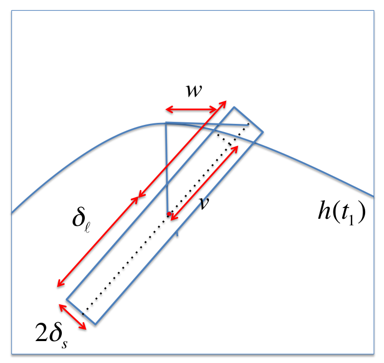
where θ\theta, δℓ\delta_{\ell}, and δs\delta_{s} (δs≤δℓ\delta_{s}\leq\delta_{\ell}) represent the orientation angle, length, and width of the neighborhood, respectively. Figure 3 displays such neighborhoods for two different pixels. We partition Iθ,δs,δℓ​(t1,t2){I}_{\theta,\delta_{s},\delta_{\ell}}(t_{1},t_{2}) into ns×nℓn_{s}\times n_{\ell} subregions Iθ,δs,δℓj1,j2​(t1,t2)≜Rt1,t2θ​([t1−j1​δℓ2​nℓ,t1+j1​δℓ2​nℓ]×[t2−j2​δs2​ns,t2+j2​δs2​ns]){I}^{j_{1},j_{2}}_{\theta,\delta_{s},\delta_{\ell}}(t_{1},t_{2})\triangleq R^{\theta}_{t_{1},t_{2}}([t_{1}-\frac{j_{1}\delta_{\ell}}{2n_{\ell}},t_{1}+\frac{j_{1}\delta_{\ell}}{2n_{\ell}}]\times[t_{2}-\frac{j_{2}\delta_{s}}{2n_{s}},t_{2}+\frac{j_{2}\delta_{s}}{2n_{s}}]).

Refer to caption
Figure 3: The anisotropic neighborhood Iθ,δs,δℓ​(t1,t2){I}_{\theta,\delta_{s},\delta_{\ell}}(t_{1},t_{2}) in the discrete setting for two different pixels of a Horizon class image.

The pixelated neighborhood of (t1,t2)(t_{1},t_{2}) is defined as the 𝐲∈ℝns×nℓ\mathbf{y}\in\mathds{R}^{n_{s}\times n_{\ell}} satisfying

𝐲t1,t2θ,δℓ,δs​(j1,j2)≜ns​nℓδs​δℓ​∫∫(s1,s2)∈Iθ,δs,δℓj1,j2​(t1,t2)d​Y​(s1,s2).\mathbf{y}^{\theta,\delta_{\ell},\delta_{s}}_{t_{1},t_{2}}(j_{1},j_{2})\triangleq\frac{n_{s}n_{\ell}}{\delta_{s}\delta_{\ell}}\int\int_{(s_{1},s_{2})\in I^{j_{1},j_{2}}_{\theta,\delta_{s},\delta_{\ell}}(t_{1},t_{2})}dY(s_{1},s_{2}).

Define the neighborhood process as

X⁡(t1,t2)≜ns​nℓδs​δℓ​∫∫(s1,s2)∈Iθ,δsns,δℓnℓ​(t1,t2)d​Y​(s1,s2).X(t_{1},t_{2})\triangleq\frac{n_{s}n_{\ell}}{\delta_{s}\delta_{\ell}}\int\int_{(s_{1},s_{2})\in I_{\theta,\frac{\delta_{s}}{n_{s}},\frac{\delta_{\ell}}{n_{\ell}}}(t_{1},t_{2})}dY(s_{1},s_{2}).

The anisotropic (δℓ,δs,θ)(\delta_{\ell},\delta_{s},\theta)-neighborhood distance between two given points in the image is then defined as

dθ,δs,δℓ2​(d​Y​(t1,t2),d​Y​(s1,s2))\displaystyle d^{2}_{\theta,\delta_{s},\delta_{\ell}}(dY(t_{1},t_{2}),dY(s_{1},s_{2})) (8)
≜\displaystyle\triangleq 1ns​nℓ−1​(‖𝐲t1,t2θ,δℓ,δs−𝐲s1,s2θ,δℓ,δs‖22−|𝐲t1,t2θ,δℓ,δs​(0,0)−𝐲s1,s2θ,δℓ,δs​(0,0)|2).\displaystyle\!\!\!\frac{1}{n_{s}n_{\ell}-1}\left(\|\mathbf{y}^{\theta,\delta_{\ell},\delta_{s}}_{t_{1},t_{2}}-\mathbf{y}^{\theta,\delta_{\ell},\delta_{s}}_{s_{1},s_{2}}\|_{2}^{2}-|\mathbf{y}^{\theta,\delta_{\ell},\delta_{s}}_{t_{1},t_{2}}(0,0)-\mathbf{y}^{\theta,\delta_{\ell},\delta_{s}}_{s_{1},s_{2}}(0,0)|^{2}\right).

The ANLM estimate at point (t1,t2)(t_{1},t_{2}) is given by

f^θ,δs,δℓ​(t1,t2)≜∫(s1,s2)∈Swt1,t2θ,δs,δℓ​(s1,s2)​X​(s1,s2)​d​s1​d​s2∫∫(s1,s2)∈Swt1,t2θ,δs,δℓ​(s1,s2)​d​s1​d​s2.\displaystyle\hat{f}^{\theta,\delta_{s},\delta_{\ell}}(t_{1},t_{2})\triangleq\frac{\int_{(s_{1},s_{2})\in S}w^{\theta,\delta_{s},\delta_{\ell}}_{t_{1},t_{2}}(s_{1},s_{2})X(s_{1},s_{2})ds_{1}ds_{2}}{\int\int_{(s_{1},s_{2})\in S}w^{\theta,\delta_{s},\delta_{\ell}}_{t_{1},t_{2}}(s_{1},s_{2})ds_{1}ds_{2}}.

where the weights are obtained from

wt1,t2θ,δs,δℓ​(s1,s2)={1 if dθ,δs,δℓ2​(d​Y​(t1,t2),d​Y​(s1,s2))≤2​ns​nℓ​σ2δs​δℓ+τσ,0 otherwise.\displaystyle w^{\theta,\delta_{s},\delta_{\ell}}_{t_{1},t_{2}}(s_{1},s_{2})=\!\!\left\{\begin{array}[]{rl}1&\mbox{ if $d^{2}_{\theta,\delta_{s},\delta_{\ell}}(dY(t_{1},t_{2}),dY(s_{1},s_{2}))\leq\frac{2n_{s}n_{\ell}\sigma^{2}}{\delta_{s}\delta_{\ell}}+\tau_{\sigma}$,}\\ 0&\mbox{ otherwise.}\end{array}\right.

Here τσ\tau_{\sigma} is the threshold parameter and 2​ns​nℓ​σ2δs​δℓ+τσ\frac{2n_{s}n_{\ell}\sigma^{2}}{\delta_{s}\delta_{\ell}}+\tau_{\sigma} is the threshold value.

ANLM extends NLM in two significant ways. First, in ANLM θ,δs,δℓ\theta,\delta_{s},\delta_{\ell} are free parameters, while in NLM θ=0\theta=0 and δs=δℓ\delta_{s}=\delta_{\ell}. As Figures 4 and 5 demonstrate, these free parameters significantly affect the performance of ANLM. Figure 4 illustrates the visual denoising results as we vary the angle of the anisotropic neighborhood. Figure 5 does the same for the empirical peak signal-to-noise ratio (PSNR).66 6 In practice images are measured on a discrete lattice, i.e., the pixelated values are known. Let the pixelated values of the original noise-free image and the estimator be fi​jf_{ij} and f^i,j\hat{f}_{i,j}, respectively. The empirical mean-squared-error (MSE) of an estimator f^\hat{f} is defined as MSE=1n2​∑i,j(f^i,j−fi,j)2{\rm MSE}=\frac{1}{n^{2}}\sum_{i,j}(\hat{f}_{i,j}-f_{i,j})^{2}. If fi,j∈[0,A]f_{i,j}\in[0,A], then the empirical peak signal-to-noise ratio (PSNR) is defined as 10​log10​A2MSE10\log_{10}\frac{A^{2}}{\rm MSE}.

Refer to caption
(a) (a) 0∘0^{\circ}, PSNR=20.6{\rm PSNR}=20.6dB
Refer to caption
(b) (b) 45∘45^{\circ}, PSNR=19.2{\rm PSNR}=19.2dB
Refer to caption
(c) (a) 90∘90^{\circ}, PSNR=20.6{\rm PSNR}=20.6dB
Refer to caption
(d) (d) 135∘135^{\circ}, PSNR=28.9{\rm PSNR}=28.9dB
Figure 4: Effect of the anisotropic neighborhood orientation angle θ\theta on the denoising performance of ANLM. The images are 256×256256\times 256 pixels with a true edge orientation of 135∘135^{\circ}. The noise standard deviation is ξ=0.5\xi=0.5, which is equivalent to PSNR=6.1{\rm PSNR}=6.1dB (see Section 4.1). The neighborhood size and threshold parameter are δs=1/256\delta_{s}=1/256, δℓ=20/256\delta_{\ell}=20/256 and τ=2.7​ξ2\tau=2.7\xi^{2}, respectively. The angles of the neighborhoods (θ\theta) and the resulting PSNR of the estimates are noted below the images. There is a substantial subjective and objective improvement in the performance of ANLM when the neighborhood is aligned with the edge.
Figure 5: Effect of the anisotropic neighborhood orientation angle θ\theta on the denoising performance of ANLM. The experimental parameters are the same as in Figure 4. For each value of θ\theta we plot the result of 10 Monte Carlo simulations. PSNR of the original noisy image is 6.16.1dB

3.2 Oracle ANLM

It is clear from Figures 4 and 5 that we should align the ANLM neighborhood locally with the edge to maximize denoising performance. In the Oracle ANLM (OANLM) algorithm, we assume that we have access to an oracle that knows the image’s edge orientation at each pixel. Consider fh​(t1,t2)∈Hα​(C)f_{h}(t_{1},t_{2})\in H^{\alpha}(C). Let h′​(t1)h^{\prime}(t_{1}) denote the derivative of the edge contour h⁡(t1)h(t_{1}), and let Γγ≜{(t1,t2):t1=γ}{\Gamma}_{\gamma}\triangleq\{(t_{1},t_{2})\ :\ t_{1}=\gamma\} segment the region SS. Define θγ\theta_{\gamma} as the angle between the tangent to the edge contour hh and the horizontal line at t1=γt_{1}=\gamma. OANLM is defined as ANLM with the following parameter settings:

  • 1.

    Quadratic scaling: Instead of using isotropic (square) neighborhoods, we use anisotropic (rectangular) neighborhoods of size δs×δℓ\delta_{s}\times\delta_{\ell}. The scaling of δs\delta_{s} and δℓ\delta_{\ell} depends on the smoothness of the edge. Since we are primarily interested in H2​(C){H}^{2}(C), we will emphasize the quadratic scaling77 7 If the smoothness of an edge is α>1\alpha>1, then the optimal neighborhood size is given by δs=Θ⁡(σ2​α/(α+1)​|log⁡σ|OPEN2​α/(α+1))CLOSE\delta_{s}=\Theta(\sigma^{2\alpha/(\alpha+1)}|\log\sigma|^{2\alpha/(\alpha+1))} and δℓ=Θ⁡(σ2/(α+1)​|log⁡σ|2/(α+1))\delta_{\ell}=\Theta(\sigma^{2/(\alpha+1)}|\log\sigma|^{2/(\alpha+1)}). Note that for the special case α=2\alpha=2 they satisfy the quadratic scaling. δs=4​σ4/3​|log⁡σ|4/3\delta_{s}=4\sigma^{4/3}|\log{\sigma}|^{4/3} and δℓ=2​σ2/3​|log⁡σ|2/3\delta_{\ell}=2\sigma^{2/3}|\log{\sigma}|^{2/3}; that is δs=δℓ2\delta_{s}=\delta_{\ell}^{2}.

  • 2.

    Aligned neighborhoods: We align the neighborhood at point (t1,t2)(t_{1},t_{2}) to the orientation θt1\theta_{t_{1}} of the edge contour at (t1,h⁡(t1))(t_{1},h(t_{1})). Thus all pixels in a column have the same orientation. Figure 6 illustrates such a neighborhood selection.88 8 In smooth regions, where the pixel neighborhoods do not intersect with the edge, neither the shape nor the orientation of the neighborhood affect the denoising performance.

  • 3.

    Logarithmic pixelation: We assume that ns×nℓ=⌈log2⁡σ⌉n_{s}\times n_{\ell}=\lceil\log^{2}\sigma\rceil. In other words, as σ\sigma increases the resolution of the pixelated image increases as well.

Refer to caption
Figure 6: The OANLM neighborhoods satisfy the quadratic scaling δs=δℓ2\delta_{s}=\delta_{\ell}^{2} and are aligned with the edge. In regions far from the edge, isotropic neighborhoods perform just as well.
Theorem 2.

If f^O\hat{f}^{O} is the OANLM estimator with the threshold τσ=2|log⁡σ|\tau_{\sigma}=\frac{2}{\sqrt{|\log\sigma|}}, then

R⁡(Hα​(C),f^O)=O⁡(σ4/3​|log⁡σ|4/3).\displaystyle R({H}^{\alpha}(C),\hat{f}^{O})=O(\sigma^{4/3}|\log\sigma|^{4/3}).

The proof of Theorem 2 can be simply modified to provide a bound for the risk of NLM as well. Let δ=δs​δℓ\delta=\sqrt{\delta_{s}\delta_{\ell}} and n=ns​nℓ=|log⁡(σ)|n=\sqrt{n_{s}n_{\ell}}=|\log(\sigma)|, where δs\delta_{s}, δℓ\delta_{\ell}, nsn_{s}, nℓn_{\ell} are as given in OANLM algorithm.

Corollary 1.

If f^N\hat{f}^{N} is the NLM estimator with threshold τσ=2/|log⁡(σ)|\tau_{\sigma}=2/\sqrt{|\log(\sigma)|}, then

R⁡(Hα​(C),f^N)=O⁡(σ​|log⁡σ|).\displaystyle R({H}^{\alpha}(C),\hat{f}^{N})=O(\sigma|\log\sigma|).

See Section 7.3 for the proof of this corollary. Also, under certain mild assumptions, the risk of NLM can be lower bounded by Ω⁡(σ)\Omega(\sigma). The proof is similar to the proof of Theorem 5 in Maleki et al. [2012a]. However, for the sake of completeness and since our framework differs from Maleki et al. [2012a], we overview the main steps of the proof in B.

Theorem 2 is based on the strong oracle assumption that the edge direction is known exactly. Needless to say, such information is rarely available in practical applications. Consider a weaker notion of OANLM that has access to an estimate θ^γ\hat{\theta}_{\gamma} of θγ\theta_{\gamma} that satisfies

|θ^γ−θγ|≤Θ⁡(σβ).|\hat{\theta}_{\gamma}-\theta_{\gamma}|\leq\Theta(\sigma^{\beta}). (12)

OANLM with exact edge orientation information corresponds to β=∞\beta=\infty in this model. When β<∞\beta<\infty, the choices δℓ=2​σ2/3​|log⁡σ|2/3\delta_{\ell}=2\sigma^{2/3}|\log\sigma|^{2/3} and δs=4​σ4/3​|log⁡σ|4/3\delta_{s}=4\sigma^{4/3}|\log\sigma|^{4/3} are not necessarily optimal. The following theorem characterizes the performance of OANLM using θ^\hat{\theta}.

Theorem 3.

Let the OANLM estimator use the inaccurate edge orientation θ^γ\hat{\theta}_{\gamma} satisfying (12). Set the neighborhood sizes to δℓ=min⁡(σ2/3​|log2/3⁡σ|,σ1−β/2​|log⁡σ|)\delta_{\ell}=\min(\sigma^{2/3}|\log^{2/3}\sigma|,\sigma^{1-\beta/2}|\log\sigma|) and δs=σ2​log2​σ/δℓ\delta_{s}=\sigma^{2}\log^{2}\sigma/\delta_{\ell}. Then the risk of the estimator with τσ=2/|log⁡(σ)|\tau_{\sigma}=2/\sqrt{|\log(\sigma)|} satisfies

R⁡(Hα​(C),f^O)=O⁡(δs​Poly​(|log⁡σ|)),\displaystyle R({H}^{\alpha}(C),\hat{f}^{O})=O(\delta_{s}{\rm Poly}(|\log\sigma|)),

where Poly⁡(|log⁡σ|){\rm Poly}(|\log\sigma|) is a polynomial of degree at most 22 in terms of |log⁡σ||\log\sigma|.

If the edge estimate is exact, then the result simplifies to the result of Theorem 2. However, this theorem confirms that OANLM algorithm achieves the optimal rate even if there is an error in θ^\hat{\theta} of order O⁡(σβ)O(\sigma^{\beta}) with β≥2/3\beta\geq 2/3.

Corollary 2.

Let the OANLM estimator use the inaccurate edge orientation θ^γ\hat{\theta}_{\gamma} satisfying (12) with β≥2/3\beta\geq 2/3. Set the neighborhood sizes to δℓ=2​σ2/3​|log2/3⁡σ|\delta_{\ell}=2\sigma^{2/3}|\log^{2/3}\sigma| and δs=4​σ4/3​|log⁡σ|\delta_{s}=4\sigma^{4/3}|\log\sigma|. Then, the risk of the estimator with τσ=2/|log⁡(σ)|\tau_{\sigma}=2/\sqrt{|\log(\sigma)|} satisfies

R⁡(Hα​(C),f^O)=O⁡(σ4/3​Poly​(|log⁡σ|)),\displaystyle R({H}^{\alpha}(C),\hat{f}^{O})=O(\sigma^{4/3}{\rm Poly}(|\log\sigma|)),

where Poly⁡(|log⁡σ|){\rm Poly}(|\log\sigma|) is a polynomial of degree at most 4 in terms of |log⁡(σ)||\log(\sigma)|.

Proof.

If we plug in β≥2/3\beta\geq 2/3 in Theorem 3 we obtain

δℓ=min⁡(2​σ2/3​|log2/3⁡σ|,2​σ1−β/2​|log⁡σ|)=2​σ2/3​|log⁡σ|2/3.\delta_{\ell}=\min(2\sigma^{2/3}|\log^{2/3}\sigma|,2\sigma^{1-\beta/2}|\log\sigma|)=2\sigma^{2/3}|\log\sigma|^{2/3}.

Therefore, δs=4​σ4/3​|log⁡σ|4/3\delta_{s}=4\sigma^{4/3}|\log\sigma|^{4/3}. This establishes the result. ∎

We can also simplify the result of Theorem 3 for the case of β<2/3\beta<2/3.

Corollary 3.

Let the OANLM estimator use the inaccurate edge orientation θ^γ\hat{\theta}_{\gamma} satisfying (12) with β≤2/3\beta\leq 2/3. Set the neighborhood sizes to δℓ=2​σ1−β/2​|log⁡σ|\delta_{\ell}=2\sigma^{1-\beta/2}|\log\sigma| and δs=4​σ1+β/2​|log⁡σ|\delta_{s}=4\sigma^{1+\beta/2}|\log\sigma|. Then, the risk of the estimator with τσ=2/|log⁡(σ)|\tau_{\sigma}=2/\sqrt{|\log(\sigma)|} satisfies

R⁡(Hα​(C),f^O)=O⁡(σ1+β/2​Poly​(|log⁡σ|)).\displaystyle R({H}^{\alpha}(C),\hat{f}^{O})=O(\sigma^{1+\beta/2}{\rm Poly}(|\log\sigma|)).

where Poly⁡(|log⁡σ|){\rm Poly}(|\log\sigma|) is a polynomial of degree at most 3 in terms of |log⁡(σ)||\log(\sigma)|.

Proof.

Note that this corollary is exactly the same as Theorem 3. In fact, since β≤2/3\beta\leq 2/3,

δℓ=min⁡(σ2/3​|log2/3⁡σ|,σ1−β/2​|log⁡σ|)=σ1−β/2​|log⁡σ|.\delta_{\ell}=\min(\sigma^{2/3}|\log^{2/3}\sigma|,\sigma^{1-\beta/2}|\log\sigma|)=\sigma^{1-\beta/2}|\log\sigma|.

Therefore, δs=σ1+β/2​|log⁡σ|\delta_{s}=\sigma^{1+\beta/2}|\log\sigma| and therefore, according to Theorem 3

R⁡(Hα​(C),f^O)=O⁡(σs​Poly​(|log⁡σ|))=O⁡(σ1+β/2​Poly​(|log⁡σ|)).\displaystyle R({H}^{\alpha}(C),\hat{f}^{O})=O(\sigma_{s}{\rm Poly}(|\log\sigma|))=O(\sigma^{1+\beta/2}{\rm Poly}(|\log\sigma|)).

∎

This corollary suggests that, as long as we have an edge orientation estimate that improves as σ→0\sigma\rightarrow 0 (or the number of pixels increases), OANLM outperforms NLM. Also note that, as β\beta decreases, the neighborhoods become more isotropic.

3.3 Discrete angle ANLM

In this section, we introduce the Discrete-angle ANLM (DANLM) algorithm that achieves the minimax rate without oracle information. The key idea is to calculate the neighborhood distance over several directional neighborhoods and fuse them to obtain a similarity measure that works well for all directions. As for OANLM, set δs=4​σ4/3​|log⁡(σ)|4/3\delta_{s}=4\sigma^{4/3}|\log(\sigma)|^{4/3} and δℓ=2​σ2/3​|log⁡(σ)|2/3\delta_{\ell}=2\sigma^{2/3}|\log(\sigma)|^{2/3}, and let q≜πσ−2/3q\triangleq\pi\sigma^{-2/3}. Define the angles θ0≜0\theta_{0}\triangleq 0, θ1≜σ2/3\theta_{1}\triangleq\sigma^{2/3}, θ2≜2​σ2/3,…,θq≜π−σ2/3\theta_{2}\triangleq 2\sigma^{2/3},\ldots,\theta_{q}\triangleq\pi-\sigma^{2/3} and

𝒪≜{θ0,…,θq}.\mathcal{O}\triangleq\{\theta_{0},\ldots,\theta_{q}\}.

For a point (u,v)(u,v) we consider all of the anisotropic, directional neighborhoods for θ∈𝒪\theta\in\mathcal{O}. Figure 7 displays four of these neighborhoods.

Refer to caption
Figure 7: DANLM neighborhoods around one pixel location for q=4q=4.

Define the discrete angle anisotropic distance between d​Y​(t1,t2)dY(t_{1},t_{2}) and d​Y​(s1,s2)dY(s_{1},s_{2}) as

d𝒜2​(d​Y​(t1,t2),d​Y​(s1,s2))≜minθ∈𝒪⁡dθ,δs,δℓ2​(d​Y​(t1,t2),d​Y​(s1,s2)),d_{\mathcal{A}}^{2}(dY(t_{1},t_{2}),dY(s_{1},s_{2}))\triangleq\min_{\theta\in\mathcal{O}}d_{\theta,\delta_{s},\delta_{\ell}}^{2}(dY(t_{1},t_{2}),dY(s_{1},s_{2})),

where dθ,δs,δℓ2​(d​Y​(t1,t2),d​Y​(s1,s2))d_{\theta,\delta_{s},\delta_{\ell}}^{2}(dY(t_{1},t_{2}),dY(s_{1},s_{2})) is defined in (8). The DANLM estimate is then given by

f^D​(t1,t2)=∫(s1,s2)∈Swt1,t2A​N​(s1,s2)​X​(s1,s2)​d​s1​d​s2∫(s1,s2)∈Swt1,t2A​N​(s1,s2)​d​s1​d​s2.\displaystyle\hat{f}^{D}(t_{1},t_{2})=\frac{\int_{(s_{1},s_{2})\in S}w^{AN}_{t_{1},t_{2}}(s_{1},s_{2})X(s_{1},s_{2})ds_{1}ds_{2}}{\int_{(s_{1},s_{2})\in S}w^{AN}_{t_{1},t_{2}}(s_{1},s_{2})ds_{1}ds_{2}}.

where

wt1,t2A​N​(s1,s2)={1 if d𝒜2​(d​Y​(t1,t2),d​Y​(s1,s2))≤2​ns​nℓ​σ2δs​δℓ+τσ,0 otherwise.\displaystyle w^{AN}_{t_{1},t_{2}}(s_{1},s_{2})=\!\!\left\{\begin{array}[]{rl}1&\mbox{ if $d^{2}_{\mathcal{A}}(dY(t_{1},t_{2}),dY(s_{1},s_{2}))\leq\frac{2n_{s}n_{\ell}\sigma^{2}}{\delta_{s}\delta_{\ell}}+\tau_{\sigma}$,}\\ 0&\mbox{ otherwise.}\end{array}\right.

In summary, we note the following features of the DANLM algorithm. First, it uses the quadratic scaling δs=δℓ2\delta_{s}=\delta_{\ell}^{2}. Second, the optimal neighborhood direction can change from pixel to pixel. The following theorem, proved in Section 7, shows that the risk of this algorithm is within the logarithmic factor of the optimal minimax risk.

Theorem 4.

The risk of DANLM satisfies

R⁡(Hα​(Cα),f^D)≤O⁡(σ4/3​|log⁡(σ)|4/3).R(H^{\alpha}(C_{\alpha}),\hat{f}^{D})\leq O(\sigma^{4/3}|\log(\sigma)|^{4/3}).

Figure 8 reprises the simulation experiment of Figure 4 using the four algorithms described thus far: NLM, OANLM with perfect knowledge of the edge orientation, OANLM with imperfect knowledge of the edge orientation, and DANLM with four angles. All three of the latter algorithms outperform the isotropic NLM.

Refer to caption
(a) NLM, PSNR=26{\rm PSNR}=26 dB
Refer to caption
(b) OANLM with no error,
PSNR=28.9{\rm PSNR}=28.9 dB
Refer to caption
(c) ONALM with error,
PSNR=28.6{\rm PSNR}=28.6 dB
Refer to caption
(d) DANLM, PSNR=27.5{\rm PSNR}=27.5 dB
Figure 8: Continuation of the experiment of Figure 4 that compares (a) isotropic NLM, (b) OANLM with perfect knowledge of the edge direction, (c) OANLM with 10% error in the knowledge of the edge direction, (d) DANLM with q=4q=4 angles. The images are of size 256×256256\times 256 pixels. In the ANLM algorithms, δs\delta_{s} and δℓ\delta_{\ell} are the same as in Figure 4. The neighborhood size of NLM is δs×δℓ\sqrt{\delta_{s}\times\delta_{\ell}}. The edge orientation is 135∘135^{\circ}. The standard deviation of the noise is ξ=0.5\xi=0.5 which implies PSNR=6.1​dB\rm PSNR=6.1dB.

4 Practical ANLM algorithms and experiments

In this section we introduce a practical gradient-based ANLM algorithm and then complement the above theoretical arguments with additional simulations and experiments with synthetic and real-world imagery. Note that the algorithms we introduce in this section do not immediately outperform state-of-the-art denoising algorithms such as BM3D Dabov et al. [2007] but are rather intended to highlight that anisotropic neighborhoods are more suitable for edges than isotropic ones. Since NLM is a key building block in several top-performing algorithms Dabov et al. [2007], Kervrann and Boulanger [2006], we expect that anisotropy will pay off for such algorithms as it does for NLM. But addressing this important question is left for future research.

4.1 Extension to discrete images

In practice the observations are noisy pixelated values of an image and the objective is only to estimate the pixelated values. In this section we explain how the ideas of directional neighborhood and ANLM can be extended to the discrete settings. Suppose we are interested in estimating a n×nn\times n image f⁡(in,jn)f(\frac{i}{n},\frac{j}{n}) with noisy observations oi,j=f⁡(in,jn)+ζi,jo_{i,j}=f(\frac{i}{n},\frac{j}{n})+\zeta_{i,j}, where ζi,j​∼i​i​d​N​(0,ξ2)\zeta_{i,j}\overset{iid}{\sim}N(0,\xi^{2}) and ξ\xi is the standard deviation of the noise. The extension of the anisotropic neighborhood to the discrete setting is straightforward. Let S¯≜{1n,2n,…,n−1n,1}×{1n,2n,…,n−1n,1}\bar{S}\triangleq\left\{\frac{1}{n},\frac{2}{n},\ldots,\frac{n-1}{n},1\right\}\times\left\{\frac{1}{n},\frac{2}{n},\ldots,\frac{n-1}{n},1\right\} and S~≜{1,2,…,n}×{1,2,…,n}\tilde{S}\triangleq\{1,2,\ldots,n\}\times\{1,2,\ldots,n\}. For a given set B⊂S=[0,1]2B\subset S=[0,1]^{2} we define B¯≜B∩S¯\bar{B}\triangleq B\cap\bar{S}.

The discrete (θ,δs,δℓ)(\theta,\delta_{s},\delta_{\ell})-distance between two pixels oi,jo_{i,j} and om,ℓo_{m,\ell} is defined as

d¯θ,δs,δℓ2​(oi,j,om,ℓ)≜1|𝒫|​∑(r,q)∈𝒫(oi+r,j+q−om+r,ℓ+q)2,\displaystyle\bar{d}_{\theta,\delta_{s},\delta_{\ell}}^{2}(o_{i,j},o_{m,\ell})\triangleq\frac{1}{|\mathcal{P}|}\sum\limits_{(r,q)\in\mathcal{P}}(o_{i+r,j+q}-o_{m+r,\ell+q})^{2}, (16)

where 𝒫≜{(r,q)∈ℤ2|(i+rn,j+qn)∈I¯θ,δs,δℓ​(in,jn)}\mathcal{P}\triangleq\{(r,q)\in\mathds{Z}^{2}\ |\ (\frac{i+r}{n},\frac{j+q}{n})\in\bar{I}_{\theta,\delta_{s},\delta_{\ell}}(\frac{i}{n},\frac{j}{n})\}. See Figure 9. Note that for the pixels that are close to the image boundaries the neighborhoods are not rectangular any more and they include the part of the rectangle that is inside the image boundaries. Such non-rectangular neighborhoods will be compared with non-rectangular neighborhoods of the other pixels for the calculation of the distance. The ANLM estimate at pixel f⁡(in,jn)f(\frac{i}{n},\frac{j}{n}) is given by

Refer to caption
Figure 9: The anisotropic neighborhood I¯θ,δs,δℓ​(in,jn)\bar{I}_{\theta,\delta_{s},\delta_{\ell}}(\frac{i}{n},\frac{j}{n}) in the discrete setting for two different pixels of a Horizon class image. The bold red dots represent the anisotropic neighborhoods.
f^i,jθ,δs,δℓ≜∑m∑ℓw¯i,jθ,δℓ,δs​(m,ℓ)​om,ℓ∑m∑ℓw¯i,jθ,δℓ,δs​(m,ℓ),\displaystyle\hat{f}_{i,j}^{\theta,\delta_{s},\delta_{\ell}}\triangleq\frac{\sum_{m}\sum_{\ell}{\bar{w}}^{\theta,\delta_{\ell},\delta_{s}}_{i,j}(m,\ell)o_{m,\ell}}{\sum_{m}\sum_{\ell}{\bar{w}}^{\theta,\delta_{\ell},\delta_{s}}_{i,j}(m,\ell)},

where the weights are obtained from the distances d¯θ,δs,δℓ2​(oi,j,om,ℓ)\bar{d}_{\theta,\delta_{s},\delta_{\ell}}^{2}(o_{i,j},o_{m,\ell}). For instance, the simple policy introduced in (3.1) corresponds to

w¯i,jθ,δℓ,δs​(m,ℓ)≜{1 if d¯θ,δs,δℓ2​(oi,j,om,ℓ)≤2​ξ2+τn,0 otherwise.\displaystyle{\bar{w}}^{\theta,\delta_{\ell},\delta_{s}}_{i,j}(m,\ell)\triangleq\!\!\left\{\begin{array}[]{rl}1&\mbox{ if ${\bar{d}}_{\theta,\delta_{s},\delta_{\ell}}^{2}(o_{i,j},o_{m,\ell})\leq 2\xi^{2}+\tau_{n}$,}\\ 0&\mbox{ otherwise.}\end{array}\right.

Using the discrete anisotropic neighborhood and distance, the extensions of OANLM and DANLM to the discrete setting is straightforward.

4.2 Gradient-based ANLM

While DANLM is somewhat practical and also theoretically optimal for the Horizon class of images, its computational complexity is higher than NLM and grows linearly in the number of directions qq, where q∼o⁡(n2/3)q\sim o(n^{2/3}). As a more practical alternative, we propose Gradient based ANLM (GANLM), which adjusts the orientation of an anisotropic ANLM neighborhood using an estimate of the edge orientation provided by the image gradients. Pseudocode is given in Algorithm 1. Note that GANLM reverts back to NLM in regions with low image gradients, since they will not be “edgy” enough to benefit from the special treatment.

Algorithm 1 Gradient-based ANLM (GANLM)
 Inputs:
 f^i,j\hat{f}_{i,j} : Estimate of the image pixel
 δs×δℓ\delta_{s}\times\delta_{\ell}: Size of the neighborhood
 λ\lambda: Threshold that determines isotropic/anisotropic neighborhood selection
 Estimate image gradient (gh​(i,j),gv​(i,j))(g_{h}(i,j),g_{v}(i,j)) at each pixel (i,j)(i,j)
 for every pixel (i,j)∈I(i,j)\in I do
  g⁡(i,j)=gh2​(i,j)+gv2​(i,j)g(i,j)=\sqrt{g_{h}^{2}(i,j)+g_{v}^{2}(i,j)}
  θi,j=arctan⁡(gv​(i,j)gh​(i,j))\theta_{i,j}=\displaystyle\arctan\left(\frac{g_{v}(i,j)}{g_{h}(i,j)}\right)
  
  if gi≥λg_{i}\geq\lambda then
   Perform ANLM at pixel yi,jy_{i,j} with dδℓ,δs,θi,jd_{\delta_{\ell},\delta_{s},\theta_{i,j}}
  else
   Perform NLM at pixel yi,jy_{i,j} with δs​δℓ\sqrt{\delta_{s}\delta_{\ell}}.
  end if
 end for

There is a rich literature on robust image gradient estimation Feng and Milanfar [2002], Li and Orchard [2001], Bigun et al. [1991]. In our implementations we use the simplest method for estimating the image gradient, i.e.,

gh​(i,j)=f^i+1,j−f^i,j,\displaystyle g_{h}(i,j)=\hat{f}_{i+1,j}-\hat{f}_{i,j},
gv​(i,j)=f^i,j+1−f^i,j,\displaystyle g_{v}(i,j)=\hat{f}_{i,j+1}-\hat{f}_{i,j},

where f^​(i,j)\hat{f}(i,j) is an estimate of the image (for instance from isotropic NLM). If gh​(i,j)g_{h}(i,j) and gv​(i,j)g_{v}(i,j) are the estimated image derivatives at pixel (i,j)(i,j), then we can estimate the local orientation of an edge by θ^​(i,j)=arctan⁡(gv​(i,j)gh​(i,j))\hat{\theta}(i,j)=\arctan\!\left(\frac{g_{v}(i,j)}{g_{h}(i,j)}\right). To allay any concerns that gradient-based adaptivity is not robust to noise and errors, we recall Theorem 3, which establishes the robustness of OANLM to edge angle estimation error. For extremely noisy images, numerous heuristics are possible, including estimating the image gradients for GANLM from an isotropic NLM pilot estimate. Figure 11 builds on Figure 8 with a slightly more realistic, curved edge and demonstrates that the pilot estimate approach to GANLM performs almost as well as an oracle GANLM that has access to the edge gradient.

Refer to caption
(a) Noisy image, PSNR=16.5{\rm PSNR}=16.5dB
Refer to caption
(b) Horizon image
Refer to caption
(c) NLM, PSNR=34.4{\rm PSNR}=34.4dB
Refer to caption
(d) DANLM, PSNR=36.2{\rm PSNR}=36.2dB
Refer to caption
(e) Oracle GANLM, PSNR=38{\rm PSNR}=38dB
Refer to caption
(f) GANLM, PSNR=38{\rm PSNR}=38dB
Figure 10: Simulation experiment in the same vein as Figures 4 and 8 but with a slightly more realistic C2C^{2} curved edge. The images are of size 512×512512\times 512 pixels. In the ANLM algorithms δs\delta_{s} and δℓ\delta_{\ell} follow the quadratic scaling of Theorem 2. The neighborhood size of NLM is δs×δℓ\sqrt{\delta_{s}\times\delta_{\ell}}. The standard deviation of the noise is ξ=0.15\xi=0.15. To show the differences we have zoomed on the area represented by the red block in Figure (a).

Table 2 summarizes the performance of the algorithms introduced in this paper with that of NLM on the natural test images Barbara Bar [2011], Boats Boa [2011], and Wet Paint Wet [2011] submerged in noise of two different levels. The table enables us to draw two conclusions. First, the performance of the practical GANLM algorithm is very close to the oracle GANLM algorithm. Second these two algorithms outperform DANLM in all but one case and significantly outperform standard NLM in all cases. We use 4 discrete angles99 9 Experiments with larger qq did not differ appreciably in PSNR at this image size. in DANLM and attribute the superior performance of GANLM over DANLM to a more accurate selection of orientations.

4.3 Computational complexity of ANLM

Improving the risk performance of linear filters by nonlocal averaging is achieved at the price of higher computational cost. If |𝒫||\mathcal{P}| denotes the neighborhood size, then the computational complexity of NLM is proportional to Θ⁡(n4​|𝒫|)\Theta(n^{4}|\mathcal{P}|) as compared to Θ⁡(n2)\Theta(n^{2}) for linear filters. Such high complexity is not acceptable in many applications. Therefore, several effective methods have been proposed to reduce the computational complexity of NLM. See Buades et al. [2005], Mahmoudi and Sapiro [2005], Orchard et al. [2008], Brox et al. [2008] and the references therein for more information on the research in this direction. These approaches have reduced the computational complexity of NLM to an acceptable limit for practice.

The computational complexity of ANLM is in general higher than that of NLM. For instance, the computational complexity of the Gradient-based ANLM algorithm introduced in Section 4.2 is roughly two times that of NLM if we ignore the gradient calculation, which is Θ⁡(n2)\Theta(n^{2}). The computational complexity of DANLM is Θ⁡(q​n4​|𝒫|)\Theta(qn^{4}|\mathcal{P}|), where qq denotes the number of angles considered. Most of the approaches proposed for speeding up NLM are applicable to ANLM as well. Furthermore, due to specific structure of DANLM, in particular the overlap of the neighborhoods of each pixel, we expect to be able to reduce its computational complexity even further. But this question is left for future research.

Table 2: PSNR Performance of NLM and ANLM algorithms on three natural test images at two noise levels.
Test image Algorithm ξ=0.25{\xi=0.25}, 12.1dB ξ=0.15{\xi=0.15}, 16.5dB
Barbara NLM 22.48 25.86
DANLM 23.15 26.27
(512 x 512) Oracle GANLM 23.51 26.63
GANLM 23.50 26.60
Boats NLM 22.75 25.83
DANLM 23.45 26.45
(512 x 512) Oracle GANLM 23.88 26.45
GANLM 23.75 26.35
Wet Paint NLM 27.66 30.49
DANLM 28.41 30.75
(1024 x 1024) Oracle GANLM 29.02 31.18
GANLM 28.86 31.07
Refer to caption
(a) Barbara
Refer to caption
(b) Boats
Refer to caption
(c) Wet Paint
Figure 11: Zooms of the natural test images denoised by NLM (left) and ANLM (right) studies in Table 2. The standard deviation of the noise is ξ=0.15\xi=0.15 that implies PSNR=16.5=16.5dB.

5 Related work on anisotropic denoising

Anisotropy is a fundamental feature of real-world images. As a result, anisotropic image processing tools can be traced back at least as far as the 1970s Nagao and Matsuyama [1979]. Here, we briefly compare and contrast some of the relevant anisotrpic denoising schemes with ANLM.

Anisotropic filtering methods use a space-varying linear convolution filters to reduce blur along image edges. Toward this goal, Nagao and Matsuyama [1979] considers several different neighborhoods around a pixel and selects the most “homogeneous” neighborhood to smooth over. A more advanced version of this idea can be found in Takeda [2006], Takeda et al. [2007], Egiazarian et al. [2001]. There are major differences between such algorithms and NLM/ANLM; in particular, the estimators are local and do not exploit global similarities. See also Milanfar [2012] for a more complete overview of such algorithms and their differences with NLM/ANLM.

Anisotropic diffusion methods smooth a noisy image with a Gaussian kernel. As the standard deviation of the kernel increases, the smoothing process introduces larger bias to the edges. In Hummel and Moniot [1989], Koenderink [1984] the authors proved that the set of images derived by this approach can be viewed as the solution to the heat diffusion equation. Perona and Malik Perona and Malik [1990] noted the isotropy in the heat equation and introduced anisotropy. Their anisotropic diffusion starts with the heat equation but at every iteration exploits the gradient information of the previous estimate to increase the conductance along the edges and decrease it across the edges. See Kimmel et al. [2000], Tschumperlè [2006], Kimmel and Sochen [2002] for more recent advances in this direction. Efforts to theoretically analyze the risk of such algorithms have left many open questions remaining Arias-Castro and Donoho [2009]. It is conjectured that there is a connection between such algorithms and iteratively applying nonlinear filters such as the median filter. It is worth noting that the idea of applying an image denoising algorithm iteratively and guiding it at every iteration based on previous estimates goes back to Tukey’s twicing Tukey [1977].

Anisotropic transformations enable simple threshold based denoising algorithms. While the standard separable wavelet transform cannot exploit the smoothness of the edge contour, a menagerie of anisotropic transforms have been developed, including ridgelets Candès and Donoho [1999], curvelets Candès and Donoho [1999], wedgelets Donoho [1999], platelets Willett and Nowak [2003], Willett and Nowak [2007], shearlets Kutyniok and Labate [2007], Guo and Labate [2007], Easley et al. [2008], contourlets Do and Vetterli [2005], bandelets Pennec and Mallat [2005], Peyrè et al. [2007], and directionlets Velisavljevic et al. [2006]. As mentioned in the Introduction, among the above algorithms only wedgelets can obtain the optimal minimax risk for the Horizon class; however wedgelets are not suited to denoising textures. One promising avenue combing wavelets (for texture denoising) and wedgelets (for edge denoising) could follow the path of the image coder in Wakin et al. [2006]. See Laugesen et al. [2002], Jacques et al. [2011] for an overview of anisotropic transformations and their applications in image processing.

Alternative NLM algorithms have been proposed to address the inefficiency of using a fixed neighborhood Grewenig et al. [2011], Pizarro et al. [2010], Deledalle et al. [2011], Dabov et al. [2008], Salmon and Strozecki [2010], Wong et al. [2008], Kervrann and Boulanger [2006], Dabov et al. [2007]. In Deledalle et al. [2011], Salmon and Strozecki [2010], the authors aggregate several nonlocal estimates to obtain a final estimate. The nonlocal estimates are derived from NLM with different neighborhoods around each pixel. While these methods improve upon NLM on edges in practice, there is no theoretical result to support such empirical results. Similar approaches have been exploited in several state-of-the-art denoising algorithms Dabov et al. [2008], Dabov et al. [2007]. In Wong et al. [2008], Kervrann and Boulanger [2006], Van De Ville and Kocher [2009], the authors adapt the neighborhood size to the local image content. Kervrann and Boulanger [2006] considers different isotropic NLM neighborhood sizes depending on how smoothly the image content varies. Wong et al. [2008] uses image gradient information to increase the weights of the NLM along edges and decrease them across edges. This method is equivalent to modifying the threshold parameter tnt_{n} to force NLM to assign higher weights to edge-like neighborhoods. Van De Ville and Kocher [2009] sets the neighborhood size based on Stein’s unbiased estimate of the risk (SURE). Other generalizations include the rotationally invariant similarity measure Grewenig et al. [2011] and nonlocal variational approaches Pizarro et al. [2010], Gilboa and Osher [2008], Kindermann et al. [2005]. Unfortunately, these techniques do not reduce the bias that renders NLM sub-optimal.

Finally, data-driven optimality criteria have been considered in Raphan and Simoncelli [2010], Levin and Nadler [2011], Chatterjee and Milanfar [2010], where the authors derive lower bounds for the performance of denoising algorithms. However, the analyses provided in these papers are not fully rigorous and do not cover the performance of NLM for images with sharp edges.

6 Discussion and future directions

We have introduced and analyzed a framework for anisotropic nonlocal means (ANLM) denoising. Similar to NLM, ANLM exploits nonlocal information in estimating the pixel values. However, unlike NLM, ANLM uses anisotropic, oriented neighborhoods that can exploit the smoothness of edge contours. This enables ANLM to outperform NLM both theoretically and empirically. In fact, the performance of ANLM is withtin a logarithmic factor of optimal as measured by the minimax rate on the Horizon class of images.

Numerous questions remain open for future research. From the theoretical perspective, the risk analysis of GANLM, the application to noise models beyond Gaussian, and the extension to three dimensions and beyond (for seismic, medical, and other data) pose interesting research challenges. From a practical perspective, the question of how to best tune ANLM to match the nuanced edges and textures of real-world images remains open, since we have considered only brutal binary images here. Finally, while NLM is no longer the state-of-the-art denoising algorithm, it is a key building block in several top-performing algorithms. It would be interesting to see whether anisotropy pays off as handily for those algorithms as it does for NLM.

7 Proofs of the main results

7.1 Preamble

We first introduce some notation. Define the following partitions of the set S=[0,1]2S=[0,1]^{2}:

S1\displaystyle S_{1} ≜\displaystyle\triangleq {(v,u)|u>h⁡(v)+(1+C/2)​δs},\displaystyle\{(v,u)\ |\ u>h(v)+(1+C/2)\delta_{s}\},
S2\displaystyle S_{2} ≜\displaystyle\triangleq {(v,u)|h⁡(v)−(1+C/2)​δs<u<h⁡(v)+(1+C/2)​δs},\displaystyle\{(v,u)\ |\ h(v)-(1+C/2)\delta_{s}<u<h(v)+(1+C/2)\delta_{s}\},
S3\displaystyle S_{3} ≜\displaystyle\triangleq {(v,u)|u<h⁡(v)−(1+C/2)​δs}.\displaystyle\{(v,u)\ |\ u<h(v)-(1+C/2)\delta_{s}\}.

It is important to note that, if (t1,t2)∈S1(t_{1},t_{2})\in S_{1} and tan⁡(θ)=h′​(t1)\tan(\theta)=h^{\prime}(t_{1}), then Iθ,δs,δℓ​(t1,t2)I_{\theta,\delta_{s},\delta_{\ell}}(t_{1},t_{2}) does not overlap with the edge contour. In other words, the correctly aligned neighborhood of (t1,t2)∈S1(t_{1},t_{2})\in S_{1} is always above the edge. The points in S3S_{3} satisfy a similar property. This is clarified in Figure 12.

Refer to caption
Figure 12: Regions S1S_{1}, S2S_{2} and S3S_{3}. The neighborhood of (u,v)∈S3(u,v)\in{S}_{3} is aligned with the edge contour, and therefore it does not intersect the edge, while the neighborhood of (u′,v′)(u^{\prime},v^{\prime}) is not aligned and therefore may intersect with the edge. The neighborhoods of the pixels in S2S_{2} may intersect the edge even though they are correctly aligned.

We further partition S1S_{1} into P1P_{1} and P2P_{2} and S3S_{3} into P3P_{3} and P4P_{4} such that

P1\displaystyle P_{1} ≜\displaystyle\triangleq {(v,u)|h⁡(v)+2​δℓ+(C/2)​δs≤u},\displaystyle\{(v,u)\ |\ h(v)+2\delta_{\ell}+(C/2)\delta_{s}\leq u\},
P2\displaystyle P_{2} ≜\displaystyle\triangleq {(v,u)|h⁡(v)+(1+C/2)​δs≤u≤h⁡(v)+2​δℓ+(C/2)​δs},\displaystyle\{(v,u)\ |\ h(v)+(1+C/2)\delta_{s}\leq u\leq h(v)+2\delta_{\ell}+(C/2)\delta_{s}\},
P3\displaystyle P_{3} ≜\displaystyle\triangleq {(v,u)|h⁡(v)−(1+C/2)​δs≥u≥h⁡(v)−2​δℓ−(C/2)​δs},\displaystyle\{(v,u)\ |\ h(v)-(1+C/2)\delta_{s}\geq u\geq h(v)-2\delta_{\ell}-(C/2)\delta_{s}\},
P4\displaystyle P_{4} ≜\displaystyle\triangleq {(v,u)|u≤h⁡(v)−2​δℓ−(C/2)​δs}.\displaystyle\{(v,u)\ |\ u\leq h(v)-2\delta_{\ell}-(C/2)\delta_{s}\}.
Refer to caption
Figure 13: The regions P1P_{1}, P2P_{2}, P3P_{3}, P4P_{4} with αs=(1+C/2)​δs\alpha_{s}=(1+C/2)\delta_{s} and αℓ=2​δℓ−δs\alpha_{\ell}=2\delta_{\ell}-\delta_{s}. Every neighborhood of (t1,t2)∈P1(t_{1},t_{2})\in P_{1} will lie completely above the edge contour. However, some of the neighborhoods of the pixels (t1,t2)∈P2(t_{1},t_{2})\in{P}_{2} may intersect the edge. A similar property holds for the regions P3P_{3} and P4P_{4}.
Lemma 1.

Any neighborhood of pixel (v,u)∈P1(v,u)\in P_{1} will lie completely above the edge contour.

Proof.

Let (t1,t2)∈P1(t_{1},t_{2})\in P_{1}. If (u,v)∈Iθ,δs,δℓ​(t1,t2)(u,v)\in I_{\theta,\delta_{s},\delta_{\ell}}(t_{1},t_{2}), then

t2−v<δℓ.t_{2}-v<\delta_{\ell}. (20)

On the other hand, for t1′∈[t1−δℓ,t1+δℓ]t_{1}^{\prime}\in[t_{1}-\delta_{\ell},t_{1}+\delta_{\ell}] we have,

h⁡(t1′)=h⁡(t1)+h′​(t1)​(t1′−t1)+12​h′′​(t1′′)​(t1′−t1)2,h(t^{\prime}_{1})=h(t_{1})+h^{\prime}(t_{1})(t^{\prime}_{1}-t_{1})+\frac{1}{2}h^{\prime\prime}(t^{\prime\prime}_{1})(t^{\prime}_{1}-t_{1})^{2},

where t1′′t^{\prime\prime}_{1} is between t1t_{1} and t1′t^{\prime}_{1}. According to the definition of the Horizon class, h∈H​o¨​𝑙𝑑𝑒𝑟α​(C)h\in{\sl H\ddot{o}lder}^{\alpha}(C) and hence |h′​(t1)|≤1|h^{\prime}(t_{1})|\leq 1. Therefore,

h⁡(t1′)−h⁡(t1)<δℓ+12​C​δs,h(t^{\prime}_{1})-h(t_{1})<\delta_{\ell}+\frac{1}{2}C\delta_{s}, (21)

Comparing (20) and (21) completes the proof. ∎

In spite of P1P_{1}, some of the neighborhoods of the pixels (v,u)∈P2(v,u)\in P_{2} may intersect the edge. Similarly one can prove that any neighborhood of a pixel (v,u)∈P4(v,u)\in P_{4} lies completely below the edge, and some of the neighborhoods of the pixel (v,u)∈P3(v,u)\in P_{3} may intersect the edge. Figure 13 displays these regions. The following lemma, proved in Maleki et al. [2012a], will be used in the proofs of the main theorems. For the sake of completeness, we sketch the proof here.

Lemma 2.

Let Z1,Z2,…,ZrZ_{1},Z_{2},\ldots,Z_{r} be iid N⁡(0,1)N(0,1) random variables. The χr2\chi^{2}_{r} random variable ∑i=1rZi2\sum_{i=1}^{r}Z_{i}^{2} concentrates around its mean with high probability, i.e.,

ℙ⁡(1r​∑iZi2−1>t)≤e−r2​(t−ln⁡(1+t)),\displaystyle\mathds{P}\left(\frac{1}{r}\sum_{i}Z_{i}^{2}-1>t\right)\leq{\rm e}^{-\frac{r}{2}(t-\ln(1+t))}, (22)
ℙ⁡(1r​∑iZi2−1<−t)≤e−r2​(t+ln⁡(1−t)).\displaystyle\mathds{P}\left(\frac{1}{r}\sum_{i}Z_{i}^{2}-1<-t\right)\leq{\rm e}^{-\frac{r}{2}(t+\ln(1-t))}. (23)
Proof.

Here we prove (22); the proof of (23) follows along very similar lines. From Markov’s Inequality, we have

ℙ⁡((1r​∑i=1rZi2)−1>t)≤e−η​t−η​𝔼​(eηr​∑i=1rZi2)\displaystyle\mathds{P}\left(\left(\frac{1}{r}\sum_{i=1}^{r}Z_{i}^{2}\right)-1>t\right)\leq{\rm e}^{-\eta t-\eta}\mathds{E}\left({\rm e}^{\frac{\eta}{r}\sum_{i=1}^{r}Z_{i}^{2}}\right) (24)
=\displaystyle= e−η​t−η​(𝔼⁡(eη​Z12r))r=e−η​t−η(1−2​ηr)r2.\displaystyle{\rm e}^{-\eta t-\eta}\left(\mathds{E}\left({\rm e}^{\frac{\eta Z_{1}^{2}}{r}}\right)\right)^{r}=\frac{{\rm e}^{-\eta t-\eta}}{\left(1-\frac{2\eta}{r}\right)^{\frac{r}{2}}}.\hskip 56.9055pt

The last inequality follows from Lemma 3 in Maleki et al. [2012a]. The upper bound proved above holds for any η<r2\eta<\frac{r}{2}. To obtain the lowest upper bound we minimize e−η​t−η(1−2​ηr)r2\frac{{\rm e}^{-\eta t-\eta}}{\left(1-\frac{2\eta}{r}\right)^{\frac{r}{2}}} over η\eta. The optimal value is η⋆=arg⁡minη⁡e−η​t−η(1−2​ηr)r2=r​t2​(t+1)\eta^{\star}=\arg\min_{\eta}\frac{{\rm e}^{-\eta t-\eta}}{\left(1-\frac{2\eta}{r}\right)^{\frac{r}{2}}}=\frac{rt}{2(t+1)}. Plugging η⋆\eta^{\star} into (24) proves the lemma. ∎

7.2 Proof of Theorem 2

In the set up above, we consider three different regions for the point (t1,t2)(t_{1},t_{2}). As we will see in the proof, the risk of all pixels in each region has the same upper bound. We calculate these upper bounds and then combine them to obtain a master upper bound for the risk of OANLM.

Case I: (t1,t2)∈S1(t_{1},t_{2})\in S_{1}. We know that if the anisotropic neighborhood of (t1,t2)(t_{1},t_{2}), Iθ,δs,δℓI_{\theta,\delta_{s},\delta_{\ell}} is aligned with the edge contour, i.e., tan⁡(θ)=h′​(t1)\tan(\theta)=h^{\prime}(t_{1}), then it does not intersect the edge contour. To calculate the OANLM estimate we first calculate the weights. Define

𝐳t1,t2θ,δs,δℓ​(j1,j2)≜ns​nℓδs​δℓ​∫(s1,s2)∈Iθ,δs,δℓj1,j2d​W​(s1,s2),\displaystyle\mathbf{z}^{\theta,\delta_{s},\delta_{\ell}}_{t_{1},t_{2}}(j_{1},j_{2})\triangleq\frac{n_{s}n_{\ell}}{\delta_{s}\delta_{\ell}}\int_{(s_{1},s_{2})\in I^{j_{1},j_{2}}_{\theta,\delta_{s},\delta_{\ell}}}dW(s_{1},s_{2}), (25)

and

Z⁡(t1,t2)\displaystyle Z(t_{1},t_{2}) ≜\displaystyle\triangleq ns​nℓδs​δℓ​∫∫(s1,s2)∈Iθ,δsns,δℓnℓ​(t1,t2)d​W​(s1,s2),\displaystyle\frac{n_{s}n_{\ell}}{\delta_{s}\delta_{\ell}}\int\int_{(s_{1},s_{2})\in I_{\theta,\frac{\delta_{s}}{n_{s}},\frac{\delta_{\ell}}{n_{\ell}}}(t_{1},t_{2})}dW(s_{1},s_{2}),
F⁡(t1,t2)\displaystyle F(t_{1},t_{2}) ≜\displaystyle\triangleq ns​nℓδs​δℓ​∫∫(s1,s2)∈Iθ,δsns,δℓnℓ​(t1,t2)f⁡(s1,s2)​d​s1​d​s2.\displaystyle\frac{n_{s}n_{\ell}}{\delta_{s}\delta_{\ell}}\int\int_{(s_{1},s_{2})\in I_{\theta,\frac{\delta_{s}}{n_{s}},\frac{\delta_{\ell}}{n_{\ell}}}(t_{1},t_{2})}f(s_{1},s_{2})ds_{1}ds_{2}.

For notational simplicity we will use w⁡(s1,s2)w({s_{1},s_{2}}) and 𝐳t1,t2​(j1,j2)\mathbf{z}_{t_{1},t_{2}}(j_{1},j_{2}) instead of wt1,t2θ,δs,δℓ​(s1,s2)w_{t_{1},t_{2}}^{\theta,\delta_{s},\delta_{\ell}}(s_{1},s_{2}) and 𝐳t1,t2θ,δs,δℓ​(j1,j2)\mathbf{z}^{\theta,\delta_{s},\delta_{\ell}}_{t_{1},t_{2}}(j_{1},j_{2}), respectively. Define

A1\displaystyle A_{1} ≜\displaystyle\triangleq {(u,v)∈P1|w⁡(u,v)=1},\displaystyle\{(u,v)\in P_{1}\ |\ w({u,v})=1\},
A2\displaystyle A_{2} ≜\displaystyle\triangleq {(u,v)∈P4|w⁡(u,v)=0}.\displaystyle\{(u,v)\in P_{4}\ |\ w({u,v})=0\}.

Here, let λ⁡(⋅)\lambda(\cdot) denote the Lebesgue measure of a set over ℝ2\mathds{R}^{2}.

Lemma 3.

Let δℓ=2​σ2/3​|log⁡(σ)|2/3\delta_{\ell}=2\sigma^{2/3}|\log(\sigma)|^{2/3} and δs=4​σ4/3​|log⁡(σ)|4/3\delta_{s}=4\sigma^{4/3}|\log(\sigma)|^{4/3}, ns=2​|log⁡(σ)|2/3n_{s}=2|\log(\sigma)|^{2/3} nℓ=4​|log⁡(σ)|4/3n_{\ell}=4|\log(\sigma)|^{4/3}, and τσ=2|log⁡σ|\tau_{\sigma}=\frac{2}{\sqrt{|\log\sigma|}}. Then,

ℙ⁡(λ⁡(P1)−λ⁡(A1)>ϵ)\displaystyle\mathds{P}(\lambda(P_{1})-\lambda(A_{1})>\epsilon) =\displaystyle= O⁡(σ8ϵ),\displaystyle O\left(\frac{\sigma^{8}}{\epsilon}\right),
ℙ⁡(λ⁡(P4)−λ⁡(A2)>ϵ)\displaystyle\mathds{P}(\lambda(P_{4})-\lambda(A_{2})>\epsilon) =\displaystyle= O⁡(σ8ϵ).\displaystyle O\left(\frac{\sigma^{8}}{\epsilon}\right).
Proof.

Here we prove the first expression. The proof of the second expression follows along a similar route. Let (u,v)∈P1(u,v)\in P_{1}. Since 𝐳t1,t2​(j1,j2)\mathbf{z}_{t_{1},t_{2}}(j_{1},j_{2}) is the integral of the Wiener sheet, we have 𝐳t1,t2​(j1,j2)∼N⁡(0,ns​nℓ​σ2δs​δℓ)\mathbf{z}_{t_{1},t_{2}}(j_{1},j_{2})\sim N(0,\frac{n_{s}n_{\ell}\sigma^{2}}{\delta_{s}\delta_{\ell}}). Similarly, 𝐳u,v​(j1,j2)∼N⁡(0,ns​nℓ​σ2δs​δℓ)\mathbf{z}_{u,v}(j_{1},j_{2})\sim N(0,\frac{n_{s}n_{\ell}\sigma^{2}}{\delta_{s}\delta_{\ell}}). Combining this with Lemma 2 we conclude that

ℙ⁡(dθ,δs,δℓ2​(d​Y​(t1,t2),d​Y​(u,v))−2​ns​nℓ​σ2δs​δℓ≥τσ)≤e−ns​nℓ​t24=O⁡(σ8).\displaystyle\mathds{P}\left(d^{2}_{\theta,\delta_{s},\delta_{\ell}}(dY(t_{1},t_{2}),dY(u,v))-2\frac{n_{s}n_{\ell}\sigma^{2}}{\delta_{s}\delta_{\ell}}\geq\tau_{\sigma}\right)\leq{\rm e}^{-\frac{n_{s}n_{\ell}t^{2}}{4}}=O(\sigma^{8}).

Therefore,

𝔼⁡(λ⁡(A1))\displaystyle\mathds{E}(\lambda(A_{1})) =\displaystyle= 𝔼​∫(u,v)∈P1I⁡((u,v)∈A1)=∫(u,v)∈P1ℙ⁡((u,v)∈A1)\displaystyle\mathds{E}\int_{(u,v)\in P_{1}}I((u,v)\in A_{1})=\int_{(u,v)\in P_{1}}\mathds{P}((u,v)\in A_{1}) (26)
≥\displaystyle\geq ∫(u,v)∈P1ℙ⁡(dθ,δs,δℓ2​(d​Y​(t1,t2),d​Y​(u,v))−2​ns​nℓ​σ2δs​δℓ≤τσ)\displaystyle\int_{(u,v)\in P_{1}}\mathds{P}\left(d^{2}_{\theta,\delta_{s},\delta_{\ell}}(dY(t_{1},t_{2}),dY(u,v))-2\frac{n_{s}n_{\ell}\sigma^{2}}{\delta_{s}\delta_{\ell}}\leq\tau_{\sigma}\right)
=\displaystyle= λ⁡(P1)−O⁡(σ8).\displaystyle\lambda(P_{1})-O(\sigma^{8}).

An upper bound for ℙ⁡(λ⁡(P1)−λ⁡(A1)>ϵ)\mathds{P}(\lambda(P_{1})-\lambda(A_{1})>\epsilon) using the Markov inequality yields the result

ℙ⁡(λ⁡(P1)−λ⁡(A1)>ϵ)≤𝔼⁡(λ⁡(P1)−λ⁡(A1))ϵ=O⁡(σ8ϵ).\mathds{P}(\lambda(P_{1})-\lambda(A_{1})>\epsilon)\leq\frac{\mathds{E}(\lambda(P_{1})-\lambda(A_{1}))}{\epsilon}=O\left(\frac{\sigma^{8}}{\epsilon}\right).

∎

This lemma indicates that most of the points in P1P_{1} may contribute in the estimation of (t1,t2)∈S1(t_{1},t_{2})\in S_{1} and most of the points in P4P_{4} do not contribute in the estimate. Define the event ℰ\mathcal{E} as

ℰ≜{λ(P1)−λ(A1)<σ2}∩{λ(P4)−λ(A2)<σ2}.\mathcal{E}\triangleq\{\lambda(P_{1})-\lambda(A_{1})<\sigma^{2}\}\cap\{\lambda(P_{4})-\lambda(A_{2})<\sigma^{2}\}.

Note that according to Lemma 3, ℙ⁡(ℰc)=O⁡(σ6)\mathds{P}(\mathcal{E}^{c})=O(\sigma^{6}). As we will see later this lemma simplifies the calculation of the risk dramatically. For notational simplicity we also define the following notations:

w​X​d​u​d​v\displaystyle wXdudv ≜\displaystyle\triangleq w⁡(u,v)​X​(u,v)​d​u​d​v,\displaystyle w(u,v)X(u,v)dudv,
X​d​u​d​v\displaystyle Xdudv ≜\displaystyle\triangleq X⁡(u,v)​d​u​d​v,\displaystyle X(u,v)dudv,
w​d​u​d​v\displaystyle wdudv ≜\displaystyle\triangleq w⁡(u,v)​d​u​d​v,\displaystyle w(u,v)dudv,
Z​d​u​d​v\displaystyle Zdudv ≜\displaystyle\triangleq Z⁡(u,v)​d​u​d​v,\displaystyle Z(u,v)dudv,
w​Z​d​u​d​v\displaystyle wZdudv ≜\displaystyle\triangleq w⁡(u,v)​Z​(u,v)​d​u​d​v.\displaystyle w(u,v)Z(u,v)dudv.

The risk of the OANLM estimator at (t1,t2)∈S1(t_{1},t_{2})\in S_{1} is then given by

𝔼​(∫Sw​X​𝑑u​𝑑v∫Sw​𝑑u​𝑑v)2.\mathds{E}\left(\frac{\int_{S}wXdudv}{\int_{S}wdudv}\right)^{2}.

Define U=(∫Sw​X​𝑑u​𝑑v∫Sw​𝑑u​𝑑v)2U=\left(\frac{\int_{S}wXdudv}{\int_{S}wdudv}\right)^{2}. We have

𝔼⁡(U)=𝔼⁡(U|ℰ)​ℙ​(ℰ)+𝔼⁡(U|ℰc)​ℙ​(ℰc)≤𝔼⁡(U|ℰ)​ℙ​(ℰ)+ℙ⁡(ℰc).\displaystyle\mathds{E}(U)=\mathds{E}(U\ |\ \mathcal{E})\mathds{P}(\mathcal{E})+\mathds{E}(U\ |\ \mathcal{E}^{c})\mathds{P}(\mathcal{E}^{c})\leq\mathds{E}(U\ |\ \mathcal{E})\mathds{P}(\mathcal{E})+\mathds{P}(\mathcal{E}^{c}). (27)

Lemma 3 proves that ℙ⁡(ℰc)=O⁡(σ6)\mathds{P}(\mathcal{E}^{c})=O(\sigma^{6}). Also, since for (u,v)∈A1(u,v)\in A_{1} w⁡(u,v)=1w(u,v)=1, we have

|∫P1w​X​𝑑u​𝑑v−∫P1X​𝑑u​𝑑v|\displaystyle\left|\int_{P_{1}}wXdudv-\int_{P_{1}}Xdudv\right| (28)
=\displaystyle= |∫P1w​X​𝑑u​𝑑v−∫A1w​X​𝑑u​𝑑v+∫A1X​𝑑u​𝑑v−∫P1X​𝑑u​𝑑v|\displaystyle\left|\int_{P_{1}}wXdudv-\int_{A_{1}}wXdudv+\int_{A_{1}}Xdudv-\int_{P_{1}}Xdudv\right|
=\displaystyle= |∫P1w​X​𝑑u​𝑑v−∫A1w​X​𝑑u​𝑑v|+|∫A1X​𝑑u​𝑑v−∫P1X​𝑑u​𝑑v|\displaystyle\left|\int_{P_{1}}wXdudv-\int_{A_{1}}wXdudv\right|+\left|\int_{A_{1}}Xdudv-\int_{P_{1}}Xdudv\right|
=\displaystyle= O⁡(λ⁡(P1\A1)).\displaystyle O(\lambda(P_{1}\backslash A_{1})).

For the last inequality we have assumed that the estimate is bounded over the P1P_{1} region. This assumption can be also justified by calculating the probability that this condition does not hold and showing that the probability is negligible. Using arguments similar to (28) it is straightforward to prove that

|∫P4w​X​𝑑u​𝑑v|=O⁡(λ⁡(P4\A2)).\displaystyle\left|\int_{P_{4}}wXdudv\right|=O(\lambda(P_{4}\backslash A_{2})).
|∫P1w​𝑑u​𝑑v−∫P1d​u​𝑑v|=O⁡(λ⁡(P1\A1)).\displaystyle\left|\int_{P_{1}}wdudv-\int_{P_{1}}dudv\right|=O(\lambda(P_{1}\backslash A_{1})).
|∫P4w​𝑑u​𝑑v|=O⁡(λ⁡(P4\A2)).\displaystyle\left|\int_{P_{4}}wdudv\right|=O(\lambda(P_{4}\backslash A_{2})). (29)

Define P14≜P1∪P4P_{14}\triangleq P_{1}\cup P_{4} and B≜S\P14B\triangleq S\backslash P_{14}. We now calculate an upper bound for the first term of (41)

𝔼⁡(U|ℰ)​ℙ​(ℰ)\displaystyle\mathds{E}(U\ |\ \mathcal{E})\mathds{P}(\mathcal{E}) (30)
=(a)\displaystyle\overset{\rm(a)}{=} 𝔼⁡((∫P14w​X​𝑑u​𝑑v+∫Bw​X​𝑑u​𝑑v∫P14w​𝑑u​𝑑v+∫Bw​𝑑u​𝑑v)2|ℰ)​ℙ​(ℰ)\displaystyle\mathds{E}\left(\left(\frac{\int_{P_{14}}wXdudv+\int_{B}wXdudv}{\int_{P_{14}}wdudv+\int_{B}wdudv}\right)^{2}\ \Big|\ \mathcal{E}\right)\mathds{P}(\mathcal{E})
=\displaystyle= 𝔼⁡((∫P1X​𝑑u​𝑑v+∫Bw​X​𝑑u​𝑑v∫P1d​u​𝑑v+∫Bw​𝑑u​𝑑v)2|ℰ)​ℙ​(ℰ)+O⁡(σ2)\displaystyle\mathds{E}\left(\left(\frac{\int_{P_{1}}Xdudv+\int_{B}wXdudv}{\int_{P_{1}}dudv+\int_{B}wdudv}\right)^{2}\ \Big|\ \mathcal{E}\right)\mathds{P}(\mathcal{E})+O(\sigma^{2})
≤\displaystyle\leq 𝔼​(∫P1X​𝑑u​𝑑v+∫Bw​X​𝑑u​𝑑v∫P1d​u​𝑑v+∫Bw​𝑑u​𝑑v)2+O⁡(σ2)\displaystyle\mathds{E}\left(\frac{\int_{P_{1}}Xdudv+\int_{B}wXdudv}{\int_{P_{1}}dudv+\int_{B}wdudv}\right)^{2}+O(\sigma^{2})
≤(b)\displaystyle\overset{\rm(b)}{\leq} 𝔼​(∫Bw​F​𝑑u​𝑑v∫P1d​u​𝑑v+∫Bw​𝑑u​𝑑v)2+𝔼​(∫P1Z​𝑑u​𝑑v+∫Bw​Z​𝑑u​𝑑v∫P1d​u​𝑑v+∫Bw​𝑑u​𝑑v)2\displaystyle\mathds{E}\left(\frac{\int_{B}wFdudv}{\int_{P_{1}}dudv+\int_{B}wdudv}\right)^{2}+\mathds{E}\left(\frac{\int_{P_{1}}Zdudv+\int_{B}wZdudv}{\int_{P_{1}}dudv+\int_{B}wdudv}\right)^{2}
+ 2​𝔼​(∫Bw​F​𝑑u​𝑑v∫P1d​u​𝑑v+∫Bw​𝑑u​𝑑v)2​𝔼​(∫P1Z​𝑑u​𝑑v+∫Bw​Z​𝑑u​𝑑v∫P1d​u​𝑑v+∫Bw​𝑑u​𝑑v)2\displaystyle\!\!\!\!+\,2\sqrt{\mathds{E}\left(\frac{\int_{B}wFdudv}{\int_{P_{1}}dudv+\int_{B}wdudv}\right)^{2}}\sqrt{\mathds{E}\left(\frac{\int_{P_{1}}Zdudv+\int_{B}wZdudv}{\int_{P_{1}}dudv+\int_{B}wdudv}\right)^{2}}
+O⁡(σ2).\displaystyle\!\!\!\!+\,O(\sigma^{2}).

Equality (a) is an application of (28) and (29). To obtain (b) we plug in the value of X=F+ZX=F+Z, where FF and ZZ represent signal and noise respectively. In the next two lemmas, Lemma 30 and Lemma 5, we obtain upper bounds for individual terms in (30).

Lemma 4.

Let w⁡(u,v)w({u,v}) be the weights of OANLM with δℓ,δs,ns,nℓ\delta_{\ell},\delta_{s},n_{s},n_{\ell}, and τσ\tau_{\sigma} as specified in Lemma 3. Then

𝔼​(∫Bw​F​𝑑u​𝑑v∫P1d​u​𝑑v+∫Bw​𝑑u​𝑑v)2≤O⁡(σ4/3​|log⁡(σ)|4/3).\displaystyle\mathds{E}\left(\frac{\int_{B}wFdudv}{\int_{P_{1}}dudv+\int_{B}wdudv}\right)^{2}\leq O(\sigma^{4/3}|\log(\sigma)|^{4/3}).
Proof.

We have

𝔼​(∫Bw​F​𝑑u​𝑑v∫P1d​u​𝑑v+∫Bw​𝑑u​𝑑v)2​≤(a)​𝔼​(∫Bd​u​𝑑v∫P1d​u​𝑑v)2\displaystyle\mathds{E}\left(\frac{\int_{B}wFdudv}{\int_{P_{1}}dudv+\int_{B}wdudv}\right)^{2}\overset{(a)}{\leq}\mathds{E}\left(\frac{\int_{B}dudv}{\int_{P_{1}}dudv}\right)^{2}
=\displaystyle= (λ⁡(B)λ⁡(P1))2=O⁡(σ4/3​|log⁡(σ)|4/3).\displaystyle\left(\frac{\lambda(B)}{\lambda(P_{1})}\right)^{2}=O(\sigma^{4/3}|\log(\sigma)|^{4/3}).

To obtain Inequality (a)(a) we maximize the numerator and minimize the denominator independently. The last equality is due to the fact that λ⁡(B)=O⁡(δℓ)\lambda(B)=O(\delta_{\ell}). ∎

Lemma 5.

Let w⁡(u,v)w({u,v}) be the weights of OANLM with δℓ,δs,ns,nℓ\delta_{\ell},\delta_{s},n_{s},n_{\ell}, and τσ\tau_{\sigma} as specified in Lemma 3. Then

𝔼​(∫P1Z​𝑑u​𝑑v+∫Bw​Z​𝑑u​𝑑v∫P1d​u​𝑑v+∫Bw​𝑑u​𝑑v)2≤O⁡(σ4/3​|log⁡(σ)|4/3).\displaystyle\mathds{E}\left(\frac{\int_{P_{1}}Zdudv+\int_{B}wZdudv}{\int_{P_{1}}dudv+\int_{B}wdudv}\right)^{2}\leq O(\sigma^{4/3}|\log(\sigma)|^{4/3}).
Proof.

Since ∫Bw​𝑑u​𝑑v≥0\int_{B}wdudv\geq 0, and we are interested in the upper bound of the risk, we can remove it from the denominator to obtain

𝔼​(∫P1Z​𝑑u​𝑑v+∫Bw​Z​𝑑u​𝑑v∫P1d​u​𝑑v+∫Bw​𝑑u​𝑑v)2≤𝔼​(∫P1Z​𝑑u​𝑑v+∫Bw​Z​𝑑u​𝑑v∫P1d​u​𝑑v)2\displaystyle\mathds{E}\left(\frac{\int_{P_{1}}Zdudv+\int_{B}wZdudv}{\int_{P_{1}}dudv+\int_{B}wdudv}\right)^{2}\leq\mathds{E}\left(\frac{\int_{P_{1}}Zdudv+\int_{B}wZdudv}{\int_{P_{1}}dudv}\right)^{2}
≤\displaystyle\leq 𝔼​(∫P1Z​𝑑u​𝑑v∫P1d​u​𝑑v)2⏟V1+𝔼​(∫Bw​Z​𝑑u​𝑑v∫P1d​u​𝑑v)2⏟V2\displaystyle\underbrace{\mathds{E}\left(\frac{\int_{P_{1}}Zdudv}{\int_{P_{1}}dudv}\right)^{2}}_{V_{1}}+\underbrace{\mathds{E}\left(\frac{\int_{B}wZdudv}{\int_{P_{1}}dudv}\right)^{2}}_{V_{2}}
+ 2​𝔼​(∫P1Z​𝑑u​𝑑v∫P1d​u​𝑑v)2​𝔼​(∫Bw​Z​𝑑u​𝑑v(∫P1d​u​𝑑v)2)2⏟V3.\displaystyle+\underbrace{\ 2\sqrt{\mathds{E}\left(\frac{\int_{P_{1}}Zdudv}{\int_{P_{1}}dudv}\right)^{2}}\sqrt{\mathds{E}\left(\frac{\int_{B}wZdudv}{\left(\int_{P_{1}}dudv\right)^{2}}\right)^{2}}}_{V_{3}}.

Now we obtain upper bounds for V1V_{1},V2V_{2}, and V3V_{3} separately. First, we have

V1\displaystyle V_{1} =\displaystyle= 𝔼​(∫P1Z​𝑑u​𝑑v∫P1d​u​𝑑v)2=𝔼⁡(∫P1∫P1Z⁡(u,v)​Z​(u′,v′)​d​u′​d​v′​𝑑u​𝑑v(∫P1d​u​𝑑v)2)\displaystyle\mathds{E}\left(\frac{\int_{P_{1}}Zdudv}{\int_{P_{1}}dudv}\right)^{2}=\mathds{E}\left(\frac{\int_{P_{1}}\int_{P_{1}}Z(u,v)Z(u^{\prime},v^{\prime})du^{\prime}dv^{\prime}dudv}{\left(\int_{P_{1}}dudv\right)^{2}}\right) (31)
=(b)\displaystyle\overset{(b)}{=} (∫P1∫Iθ,2​δsns,2​δℓnℓ​(u,v)𝔼⁡(Z⁡(u,v)​Z​(u′,v′))​d​u′​d​v′​𝑑u​𝑑v(∫P1d​u​𝑑v)2)\displaystyle\left(\frac{\int_{P_{1}}\int_{I_{\theta,\frac{2\delta_{s}}{n_{s}},\frac{2\delta_{\ell}}{n_{\ell}}}(u,v)}\mathds{E}(Z(u,v)Z(u^{\prime},v^{\prime}))du^{\prime}dv^{\prime}dudv}{\left(\int_{P_{1}}dudv\right)^{2}}\right)
≤(c)\displaystyle\overset{(c)}{\leq} (∫P1∫Iθ,2​δsns,2​δℓnℓ​(u,v)ns​nℓ​σ2δs​δℓ​d​u′​d​v′​𝑑u​𝑑v(∫P1d​u​𝑑v)2)=O⁡(σ2).\displaystyle\left(\frac{\int_{P_{1}}\int_{I_{\theta,\frac{2\delta_{s}}{n_{s}},\frac{2\delta_{\ell}}{n_{\ell}}}(u,v)}\frac{n_{s}n_{\ell}\sigma^{2}}{\delta_{s}\delta_{\ell}}du^{\prime}dv^{\prime}dudv}{\left(\int_{P_{1}}dudv\right)^{2}}\right)=O\left(\sigma^{2}\right).

Equality (b) is due to the fact that if (u′,v′)∉Iθ,2​δsns,2​δℓnℓ​(u,v)(u^{\prime},v^{\prime})\notin I_{\theta,\frac{2\delta_{s}}{n_{s}},\frac{2\delta_{\ell}}{n_{\ell}}}(u,v) then Z⁡(u,v)Z(u,v) and Z⁡(u′,v′)Z(u^{\prime},v^{\prime}) will be independent and hence 𝔼⁡(Z⁡(u,v)​Z​(u′,v′))=0\mathds{E}(Z(u,v)Z(u^{\prime},v^{\prime}))=0. Inequality (c) is due to the Cauchy-Schwartz inequality |𝔼⁡(Z⁡(u,v)​Z​(u′,v′))|≤𝔼​Z2​(u,v)​𝔼​Z2​(u′,v′)|\mathds{E}(Z(u,v)Z(u^{\prime},v^{\prime}))|\leq\sqrt{\mathds{E}Z^{2}(u,v)}\sqrt{\mathds{E}Z^{2}(u^{\prime},v^{\prime})}.

To obtain an upper bound for V2V_{2}, we first note that

𝔼⁡(w⁡(u,v)​Z​(u,v)​w​(u′,v′)​Z​(u′,v′))\displaystyle\mathds{E}(w(u,v)Z(u,v)w(u^{\prime},v^{\prime})Z(u^{\prime},v^{\prime})) (32)
≤\displaystyle\leq 𝔼​(w⁡(u,v)​Z​(u,v))2​𝔼​(w⁡(u′,v′)​Z​(u′,v′))2=ns​nℓ​σ2δs​δℓ,\displaystyle\sqrt{\mathds{E}(w(u,v)Z(u,v))^{2}}\sqrt{\mathds{E}(w(u^{\prime},v^{\prime})Z(u^{\prime},v^{\prime}))^{2}}=\frac{n_{s}n_{\ell}\sigma^{2}}{\delta_{s}\delta_{\ell}},

and hence,

V2\displaystyle V_{2} =\displaystyle= 𝔼​(∫Bw​Z​𝑑u​𝑑v∫P1d​u​𝑑v)2\displaystyle\mathds{E}\left(\frac{\int_{B}wZdudv}{\int_{P_{1}}dudv}\right)^{2} (33)
=\displaystyle= 𝔼⁡(∫B∫Bw⁡(u,v)​Z​(u,v)​w​(u′,v′)​Z​(u′,v′)​𝑑u​𝑑v​d​u′​d​v′(∫P1d​u​𝑑v)2)\displaystyle\mathds{E}\left(\frac{\int_{B}\int_{B}w(u,v)Z(u,v)w(u^{\prime},v^{\prime})Z(u^{\prime},v^{\prime})dudvdu^{\prime}dv^{\prime}}{(\int_{P_{1}}dudv)^{2}}\right)
≤\displaystyle\leq (∫B∫Bns​nℓ​σ2δs​δℓ​𝑑u​𝑑v​d​u′​d​v′(∫P1d​u​𝑑v)2)=O⁡(δℓ2).\displaystyle\left(\frac{\int_{B}\int_{B}\frac{n_{s}n_{\ell}\sigma^{2}}{\delta_{s}\delta_{\ell}}dudvdu^{\prime}dv^{\prime}}{\left(\int_{P_{1}}dudv\right)^{2}}\right)=O(\delta_{\ell}^{2}).

Note that the last inequality is due to the fact that λ⁡(B)=O⁡(δℓ)\lambda(B)=O(\delta_{\ell}). Using (31) and (33) it is straightforward to obtain an upper bound for V3V_{3} by using the Cauchy-Schwartz inequality. Combining the upper bounds for V1V_{1}, V2V_{2}, and V3V_{3} completes the proof. ∎

Combining (30) with Lemmas 4 and 5 establishes the following upper bound for Case I, where (t1,t2)∈S1(t_{1},t_{2})\in S_{1}:

𝔼​(f⁡(t1,t2)−∫Sw⁡(u,v)​X​(u,v)​𝑑u​𝑑v∫Sw⁡(u,v)​𝑑u​𝑑v)2=O⁡(σ4/3​|log⁡(σ)|4/3).\displaystyle\mathds{E}\left(f(t_{1},t_{2})-\frac{\int_{S}w(u,v)X(u,v)dudv}{\int_{S}w(u,v)dudv}\right)^{2}=O(\sigma^{4/3}|\log(\sigma)|^{4/3}). (34)

Case II: (t1,t2)∈S2(t_{1},t_{2})\in S_{2}. In this case we assume that the risk is bounded by 11, since the function ff is bounded between 00 and 11. If the estimate is out of this range, then we will map it to either 00 or 11.

Case III: (t1,t2)∈S3(t_{1},t_{2})\in S_{3}. This case is exactly the same as Case I , and hence we skip the proof.

Finally, combining our results for Cases I, II, and III, we can calculate an upper bound for the risk of OANLM as

R⁡(f,f^O)\displaystyle R(f,\hat{f}^{O}) =\displaystyle= 𝔼⁡(‖f−f^O‖2)=∫S1∪S3(f−f^O)2​d​t1​d​t2+∫S2(f−f^O)2​d​t1​d​t2\displaystyle\mathds{E}(\|f-\hat{f}^{O}\|^{2})=\int_{S_{1}\cup S_{3}}(f-\hat{f}^{O})^{2}dt_{1}dt_{2}+\int_{S_{2}}(f-\hat{f}^{O})^{2}dt_{1}dt_{2}
=\displaystyle= λ⁡(S1∪S3)​O​(σ4/3​|log⁡(σ)|4/3)+λ⁡(S2)​O​(1)=O⁡(σ4/3​|log⁡(σ)|4/3).\displaystyle\lambda(S_{1}\cup S_{3})O(\sigma^{4/3}|\log(\sigma)|^{4/3})+\lambda(S_{2})O(1)=O(\sigma^{4/3}|\log(\sigma)|^{4/3}).

This ends the proof of Theorem 2.

7.3 Proof of Corollary 1

The proof of this corollary follows exactly the same route as that of Theorem 2. We merely redefine the regions SkS_{k} and PkP_{k} for k∈{1,2,3}k\in\{1,2,3\}. The new definition of the SkS_{k} regions for the NLM algorithm is given by

S1n\displaystyle S_{1}^{n} ≜\displaystyle\triangleq {(t1,t2)|t2>h⁡(t1)+2​δ},\displaystyle\{(t_{1},t_{2})\ |\ t_{2}>h(t_{1})+2\delta\},
S3n\displaystyle S_{3}^{n} ≜\displaystyle\triangleq {(t1,t2)|t2<h⁡(t1)−2​δ},\displaystyle\{(t_{1},t_{2})\ |\ t_{2}<h(t_{1})-2\delta\},

and S2n≜S\S1n∪S3nS_{2}^{n}\triangleq S\backslash S^{n}_{1}\cup S^{n}_{3}. Since the neighborhoods in NLM are isotropic, we require a single parameter to describe the neighborhood size, δ=δs=δℓ\delta=\delta_{s}=\delta_{\ell}. For notational simplicity we have assumed that C2​δ2<δ\frac{C}{2}\delta^{2}<\delta. This is a valid assumption for small enough values of σ\sigma, since δ→0\delta\rightarrow 0 as σ→0\sigma\rightarrow 0. This assumption implies that the neighborhood of the pixels in S1nS_{1}^{n} and S3nS_{3}^{n} does not intersect with the edge contour. Since the neighborhoods no longer have different anisotropic lengths, the size of the intersection of the neighborhoods and the edge contour is identical in all directions and there is no need to define the regions, P1,…,P4P_{1},\ldots,P_{4}. Equivalently, we set P1=S1nP_{1}=S_{1}^{n}, P4=S3nP_{4}=S_{3}^{n} and P2=P3=∅P_{2}=P_{3}=\emptyset. With these definitions the rest of the proof follows along the exact same lines as the proof of Theorem 2. In particular one can show that the risk of a pixel (t1,t2)∈S1n∪S3n(t_{1},t_{2})\in S_{1}^{n}\cup S_{3}^{n} is O⁡(σ2​log2⁡(σ))O(\sigma^{2}\log^{2}(\sigma)), and the risk of a point (t1,t2)∈S2n(t_{1},t_{2})\in S_{2}^{n} is O⁡(1)O(1). Furthermore, λ(S2)=O(2δ)=O(σlog(σ)|)\lambda(S_{2})=O(2\delta)=O(\sigma\log(\sigma)|). Therefore the entire risk of NLM is equal to

R⁡(f,f^N)\displaystyle R(f,\hat{f}^{N}) =\displaystyle= ∫S1∪S3(f−f^N)2​d​t1​d​t2+∫S2(f−f^N)2​d​t1​d​t2\displaystyle\int_{S_{1}\cup S_{3}}(f-\hat{f}^{N})^{2}dt_{1}dt_{2}+\int_{S_{2}}(f-\hat{f}^{N})^{2}dt_{1}dt_{2}
=\displaystyle= λ⁡(S1∪S3)​O​(σ2​log2⁡(σ))+λ⁡(S2)​O​(1)=O⁡(σ​|log⁡(σ)|).\displaystyle\lambda(S_{1}\cup S_{3})O(\sigma^{2}\log^{2}(\sigma))+\lambda(S_{2})O(1)=O(\sigma|\log(\sigma)|).

7.4 Proof of Theorem 3

The proof of this theorem is very similar to the proof of Theorem 2. The only difference is in the definitions of SkS_{k} and PkP_{k} for k∈{1,2,3}k\in\{1,2,3\}. Since there is a mismatch between the orientations of the neighborhood and the edge contour, the neighborhood of a point in S1S_{1} may intersect the edge contour. In order to fix this, we define the new regions called SiβS_{i}^{\beta} and PiβP_{i}^{\beta}. If the error in θ\theta is upper bounded by cβ​σβc_{\beta}\sigma^{\beta}, then define

S1β\displaystyle S_{1}^{\beta} ≜\displaystyle\triangleq {(t1,t2)|t2>h⁡(t1)+cβ​σβ​δℓ+δs+(C/2)​δℓ2},\displaystyle\{(t_{1},t_{2})\ |\ t_{2}>h(t_{1})+c_{\beta}\sigma^{\beta}\delta_{\ell}+\delta_{s}+(C/2)\delta_{\ell}^{2}\},
S3β\displaystyle S_{3}^{\beta} ≜\displaystyle\triangleq {(t1,t2)|t2<h⁡(t1)−cβ​σβ​δℓ−δs−(C/2)​δℓ2},\displaystyle\{(t_{1},t_{2})\ |\ t_{2}<h(t_{1})-c_{\beta}\sigma^{\beta}\delta_{\ell}-\delta_{s}-(C/2)\delta_{\ell}^{2}\},

and S2β≜S\S1β∪S3βS_{2}^{\beta}\triangleq S\backslash S^{\beta}_{1}\cup S^{\beta}_{3}. Let (t1,t2)∈S1β(t_{1},t_{2})\in S_{1}^{\beta} and set θ=arctan⁡(h′​(t1))\theta=\arctan(h^{\prime}(t_{1})). Consider a directional neighborhood of (t1,t2)(t_{1},t_{2}) with direction θ^\hat{\theta}, where |θ^−θ|≤cβ​σβ|\hat{\theta}-\theta|\leq c_{\beta}\sigma^{\beta}. Then it is straightforward to confirm that

Iθ^,δs,δℓ​(t1,t2)⊂S1β.I_{\hat{\theta},\delta_{s},\delta_{\ell}}(t_{1},t_{2})\subset S_{1}^{\beta}.

Furthermore, define P1β≜P1P_{1}^{\beta}\triangleq P_{1}, P4β≜P4P_{4}^{\beta}\triangleq P_{4}, P2β≜S1β\P1P_{2}^{\beta}\triangleq S^{\beta}_{1}\backslash P_{1}, and P3β≜S3β\P4P_{3}^{\beta}\triangleq S^{\beta}_{3}\backslash P_{4}. Note that the risk of a point (t1,t2)∈S1β(t_{1},t_{2})\in S_{1}^{\beta} can be exactly calculated as in the proof of Theorem 2 and therefore, it is upper bounded by O⁡(σ4/3​|log⁡(σ)|4/3)O(\sigma^{4/3}|\log(\sigma)|^{4/3}). Also, the risk of the pixels in S2βS_{2}^{\beta} upper bounded by O⁡(1)O(1). Finally the Lebesgue measure of S2βS_{2}^{\beta} is O⁡(cβ​σβ​δℓ+δs+(C/2)​δℓ2)O(c_{\beta}\sigma^{\beta}\delta_{\ell}+\delta_{s}+(C/2)\delta_{\ell}^{2}). Combining these facts establishes the claimed upper bound.

7.5 Proof of Theorem 4

Since the proof is mostly similar to that of Theorem 2, we shall focus on the major differences. The first difference is that we consider the regions P1P_{1}–P4P_{4} instead of S1S_{1}–S3S_{3}. Previously the regions P1P_{1} and P2P_{2} were treated jointly under the region S1S_{1}. Instead, we shall now consider P1P_{1} and P2P_{2} separately, and their differences shall become progressively apparent.

Case I: (t1,t2)∈P1(t_{1},t_{2})\in{P}_{1}. We start with the calculation of the weights w⁡(u,v)w({u,v}) for (u,v)∈P1∪P4(u,v)\in{P}_{1}\cup{P}_{4}. Define

R1≜{(u,v)∈P1|wD​(u,v)=1},\displaystyle R_{1}\triangleq\{(u,v)\in P_{1}\ |\ w^{D}({u,v})=1\},
R2≜{(u,v)∈P4|wD​(u,v)=0}.\displaystyle R_{2}\triangleq\{(u,v)\in P_{4}\ |\ w^{D}({u,v})=0\}.

Intuitively speaking, we expect most of the pixels in P1P_{1} to contribute to the estimate of the pixel at (t1,t2)(t_{1},t_{2}), since all their directional neighborhoods are very similar to the directional neighborhoods of (t1,t2)(t_{1},t_{2}). This implies that R1R_{1} is “close” to P1P_{1}. Also, we expect that most of the pixels in P4P_{4} do not contribute in the estimate since all their directional neighborhoods are different from those of (t1,t2)∈P1(t_{1},t_{2})\in P_{1}. Lemma 6 provides a formal statement of this intuition.

Lemma 6.

Let δs,δℓ,ns,nℓ,t\delta_{s},\delta_{\ell},n_{s},n_{\ell},t be as defined in Lemma 3 and let q=πσ−2/3q=\pi\sigma^{-2/3} in the DANLM algorithm. Then,

ℙ⁡(λ⁡(P1)−λ⁡(R1)>ϵ)\displaystyle\mathds{P}(\lambda(P_{1})-\lambda(R_{1})>\epsilon) ≤\displaystyle\leq O⁡(σ8ϵ),\displaystyle O\left(\frac{\sigma^{8}}{\epsilon}\right),
ℙ⁡(λ⁡(P4)−λ⁡(R2)>ϵ)\displaystyle\mathds{P}(\lambda(P_{4})-\lambda(R_{2})>\epsilon) ≤\displaystyle\leq O⁡(σ22/3ϵ).\displaystyle O\left(\frac{\sigma^{22/3}}{\epsilon}\right).
Proof.

We use the technique we developed in Lemma 3 for the proof. Consider a point (u,v)∈P1(u,v)\in P_{1} and let θ∗≜arctan⁡(h′​(t1))\theta^{*}\triangleq\arctan(h^{\prime}(t_{1})) and θ^\hat{\theta} represent an angle from 𝒪\mathcal{O} that is closest to θ∗\theta^{*}. Then,

ℙ⁡(d𝒜2​(d​Y​(t1,t2),d​Y​(u,v))−2​ns​nℓ​σ2τs​τℓ≤τσ)\displaystyle\mathds{P}\left(d^{2}_{\mathcal{A}}(dY(t_{1},t_{2}),dY(u,v))-\frac{2n_{s}n_{\ell}\sigma^{2}}{\tau_{s}\tau_{\ell}}\leq\tau_{\sigma}\right) (35)
=\displaystyle= ℙ⁡(minθ′∈𝒪⁡dθ′,δs,δℓ2​(d​Y​(t1,t2),d​Y​(u,v))−2​ns​nℓ​σ2τs​τℓ≤τσ)\displaystyle\mathds{P}\left(\min_{\theta^{\prime}\in\mathcal{O}}d^{2}_{\theta^{\prime},\delta_{s},\delta_{\ell}}(dY(t_{1},t_{2}),dY(u,v))-\frac{2n_{s}n_{\ell}\sigma^{2}}{\tau_{s}\tau_{\ell}}\leq\tau_{\sigma}\right)
≥\displaystyle\geq ℙ⁡(dθ^,δs,δℓ2​(d​Y​(t1,t2),d​Y​(u,v))−2​ns​nℓ​σ2τs​τℓ≤τσ)\displaystyle\mathds{P}\left(d^{2}_{\hat{\theta},\delta_{s},\delta_{\ell}}(dY(t_{1},t_{2}),dY(u,v))-\frac{2n_{s}n_{\ell}\sigma^{2}}{\tau_{s}\tau_{\ell}}\leq\tau_{\sigma}\right)
≥(d)\displaystyle\overset{(d)}{\geq} 1−e−ns​nℓ​τσ24=1−O⁡(σ8),\displaystyle 1-{\rm e}^{-\frac{n_{s}n_{\ell}\tau_{\sigma}^{2}}{4}}=1-O(\sigma^{8}),

where Inequality (d) is a direct consequence of Lemma 2. Again as in the proof of Lemma 3 we conclude that 𝔼⁡(λ⁡(P1)−λ⁡(R1))=O⁡(σ8)\mathds{E}(\lambda(P_{1})-\lambda(R_{1}))=O(\sigma^{8}). Employing this expression in Markov’s Inequality leads us to

ℙ⁡(λ⁡(P1)−λ⁡(R1)>ϵ)≤O⁡(σ8ϵ).\mathds{P}(\lambda(P_{1})-\lambda(R_{1})>\epsilon)\leq O\left(\frac{\sigma^{8}}{\epsilon}\right).

We now prove the second part of this lemma. Consider a point (u,v)∈P4(u,v)\in P_{4}. Then,

ℙ⁡(d𝒜2​(d​Y​(t1,t2),d​Y​(u,v))−2​ns​nℓ​σ2τs​τℓ≤τσ)\displaystyle\mathds{P}\left(d^{2}_{\mathcal{A}}(dY(t_{1},t_{2}),dY(u,v))-\frac{2n_{s}n_{\ell}\sigma^{2}}{\tau_{s}\tau_{\ell}}\leq\tau_{\sigma}\right)
=\displaystyle= ℙ⁡(minθ′∈𝒪⁡dθ′,δs,δℓ2​(d​Y​(t1,t2),d​Y​(u,v))−2​ns​nℓ​σ2τs​τℓ≤τσ)\displaystyle\mathds{P}\left(\min_{\theta^{\prime}\in\mathcal{O}}d^{2}_{\theta^{\prime},\delta_{s},\delta_{\ell}}(dY(t_{1},t_{2}),dY(u,v))-\frac{2n_{s}n_{\ell}\sigma^{2}}{\tau_{s}\tau_{\ell}}\leq\tau_{\sigma}\right)
≤\displaystyle\leq ∑i=1qℙ⁡(dθi,δs,δℓ2​(d​Y​(t1,t2),d​Y​(u,v))−2​ns​nℓ​σ2τs​τℓ≤τσ)\displaystyle\sum_{i=1}^{q}\mathds{P}\left(d^{2}_{\theta_{i},\delta_{s},\delta_{\ell}}(dY(t_{1},t_{2}),dY(u,v))-\frac{2n_{s}n_{\ell}\sigma^{2}}{\tau_{s}\tau_{\ell}}\leq\tau_{\sigma}\right)
≤\displaystyle{\leq} O⁡(σ22/3).\displaystyle O(\sigma^{22/3}).

Therefore, we conclude that 𝔼⁡(λ⁡(P4)−λ⁡(R2))=O⁡(σ22/3)\mathds{E}(\lambda(P_{4})-\lambda(R_{2}))=O(\sigma^{22/3}). Combining this with Markov’s Inequality establishes the second part of 6. ∎

Define the event ℱ\mathcal{F} as

ℱ≜{λ(P1)−λ(R1)<σ2}∩{λ(P4)−λ(R2)<σ2}.\mathcal{F}\triangleq\{\lambda(P_{1})-\lambda(R_{1})<\sigma^{2}\}\cap\{\lambda(P_{4})-\lambda(R_{2})<\sigma^{2}\}.

The risk of the OANLM estimator at (t1,t2)∈P1(t_{1},t_{2})\in P_{1} is then given by

𝔼​(∫SwA​N​X​𝑑u​𝑑v∫Sw​𝑑u​𝑑v)2.\mathds{E}\left(\frac{\int_{S}w^{AN}Xdudv}{\int_{S}wdudv}\right)^{2}.

Define U=(∫SwA​N​X​𝑑u​𝑑v∫Sw​𝑑u​𝑑v)2U=\left(\frac{\int_{S}w^{AN}Xdudv}{\int_{S}wdudv}\right)^{2}. We have

𝔼⁡(U)=𝔼⁡(U|ℱ)​ℙ​(ℱ)+𝔼⁡(U|ℱc)​ℙ​(ℱc)≤𝔼⁡(U|ℱ)​ℙ​(ℱ)+ℙ⁡(ℱc).\displaystyle\mathds{E}(U)=\mathds{E}(U\ |\ \mathcal{F})\mathds{P}(\mathcal{F})+\mathds{E}(U\ |\ \mathcal{F}^{c})\mathds{P}(\mathcal{F}^{c})\leq\mathds{E}(U\ |\ \mathcal{F})\mathds{P}(\mathcal{F})+\mathds{P}(\mathcal{F}^{c}). (36)

Lemma 6 confirms that ℙ⁡(ℱc)=O⁡(σ16/3)\mathds{P}(\mathcal{F}^{c})=O(\sigma^{16/3}). Therefore, we should obtain an upper bound for the term 𝔼⁡(U|ℱ)​ℙ​(ℱ)\mathds{E}(U\ |\ \mathcal{F})\mathds{P}(\mathcal{F}). This step of the proof is the same as the proof of Case I in Theorem 2, and therefore we do not repeat it here.

The more challenging step of the proof is to obtain an upper bound for the risk of DANLM for pixels (t1,t2)∈P2(t_{1},t_{2})\in P_{2}.

Case II: (t1,t2)∈P2(t_{1},t_{2})\in{P}_{2}. In this case we again start with defining the following two sets:

L1\displaystyle L_{1} ≜\displaystyle\triangleq {(u,v)∈P1|wu,vD=1},\displaystyle\{(u,v)\in P_{1}\ |\ w^{D}_{u,v}=1\},
L2\displaystyle L_{2} ≜\displaystyle\triangleq {(u,v)∈P4|wu,vD=0}.\displaystyle\{(u,v)\in P_{4}\ |\ w^{D}_{u,v}=0\}.

As before, our objective is to show that most of the pixels in P1P_{1} contribute in the final estimate of D​A​N​L​MDANLM and most of the pixels in P4P_{4} do not contribute. The following lemma formalizes this intuition.

Lemma 7.

Let δs,δℓ,ns,nℓ,τσ\delta_{s},\delta_{\ell},n_{s},n_{\ell},\tau_{\sigma} be as defined in Lemma 3, and let q=πσ−2/3q=\pi\sigma^{-2/3}. Then,

ℙ⁡(λ⁡(P1)−λ⁡(L1)>ϵ)\displaystyle\mathds{P}(\lambda(P_{1})-\lambda(L_{1})>\epsilon) ≤\displaystyle\leq π​σ8ϵ.\displaystyle\frac{\pi\sigma^{8}}{\epsilon}.
Proof.

We first prove that for some θ∈𝒪\theta\in\mathcal{O}, Iθ,δs,δℓ​(t1,t2)I_{\theta,\delta_{s},\delta_{\ell}}({t_{1},t_{2}}) does not intersect the edge. Suppose that θ∗\theta^{*} is such that tan⁡(θ∗)=h′​(t1)\tan(\theta^{*})=h^{\prime}(t_{1}), and consider θ^=arg⁡minθ∈𝒪​|θ−θ∗|\hat{\theta}=\arg\min_{\theta\in\mathcal{O}}|\theta-\theta^{*}|. To ensure that the neighborhood Iθ^,δs,δℓ​(t1,t2)I_{\hat{\theta},\delta_{s},\delta_{\ell}}({t_{1},t_{2}}) does not intersect with the edge, we need to have

t2+tan⁡(θ^)​(t′−t1)−δs>h⁡(t1)\displaystyle t_{2}+\tan(\hat{\theta})\left(t^{\prime}-t_{1}\right)-\delta_{s}~>~h\!\left(t_{1}\right) +\displaystyle+ h′​(t1)​(t′−t1)\displaystyle h^{\prime}\!\left(t_{1}\right)\left(t^{\prime}-t_{1}\right) (37)
+\displaystyle+ 12​h′′​(t′′)​(t′−in)2\displaystyle\frac{1}{2}h^{\prime\prime}(t^{\prime\prime})\left(t^{\prime}-\frac{i}{n}\right)^{2}

for all t′∈[t1,t1+δℓ)t^{\prime}\in[t_{1},t_{1}+\delta_{\ell}). Also, t′′∈[t1,t′]t^{\prime\prime}\in[t_{1},t^{\prime}]. According to the mean value theorem we have tan⁡(θ^)=tan⁡(θ∗)+11+tan2⁡(θ′)​Δ​θ\tan(\hat{\theta})=\tan(\theta^{*})+\frac{1}{1+\tan^{2}(\theta^{\prime})}\Delta\theta, where Δ​θ=θ^−θ∗\Delta\theta=\hat{\theta}-\theta^{*}, and θ′∈[−π/4,π/4]\theta^{\prime}\in[-\pi/4,\pi/4], since in our Horizon model we have assumed |h′​(t1)|≤1|h^{\prime}(t_{1})|\leq 1. Furthermore, |h′′​(t′′)|≤C2|h^{\prime\prime}(t^{\prime\prime})|\leq C_{2} and Δ​θ≤σ2/3≤π2​δℓ\Delta\theta\leq\sigma^{2/3}\leq\frac{\pi}{2}\delta_{\ell}. Therefore, (37) will be satisfied if

t2>h⁡(t1)+π​δℓ2​δℓ+δs+C2​δℓ2.t_{2}>h\left(t_{1}\right)+\frac{\pi\delta_{\ell}}{2}\delta_{\ell}+\delta_{s}+C_{2}\delta_{\ell}^{2}.

This constraint holds for all pixels in the region P2P_{2}. Therefore, the neighborhood Iθ^,δs,δℓ​(t1,t2)I_{\hat{\theta},\delta_{s},\delta_{\ell}}({t_{1},t_{2}}) lies completely in the region above the hh. Therefore,

ℙ⁡(d𝒜2​(d​Y​(t1,t2),d​Y​(u,v))−2​ns​nℓ​σ2τs​τℓ≤τσ)\displaystyle\mathds{P}\left(d^{2}_{\mathcal{A}}(dY(t_{1},t_{2}),dY(u,v))-\frac{2n_{s}n_{\ell}\sigma^{2}}{\tau_{s}\tau_{\ell}}\leq\tau_{\sigma}\right) (38)
=\displaystyle= ℙ⁡(minθ′∈𝒪⁡dθ′,δs,δℓ2​(d​Y​(t1,t2),d​Y​(u,v))−2​ns​nℓ​σ2τs​τℓ≤τσ)\displaystyle\mathds{P}\left(\min_{\theta^{\prime}\in\mathcal{O}}d^{2}_{\theta^{\prime},\delta_{s},\delta_{\ell}}(dY(t_{1},t_{2}),dY(u,v))-\frac{2n_{s}n_{\ell}\sigma^{2}}{\tau_{s}\tau_{\ell}}\leq\tau_{\sigma}\right)
≥\displaystyle\geq ℙ⁡(dθ^,δs,δℓ2​(d​Y​(t1,t2),d​Y​(u,v))−2​ns​nℓ​σ2τs​τℓ≤τσ)\displaystyle\mathds{P}\left(d^{2}_{\hat{\theta},\delta_{s},\delta_{\ell}}(dY(t_{1},t_{2}),dY(u,v))-\frac{2n_{s}n_{\ell}\sigma^{2}}{\tau_{s}\tau_{\ell}}\leq\tau_{\sigma}\right)
≥(e)\displaystyle\overset{(e)}{\geq} 1−e−ns​nℓ​t24=1−O⁡(σ8).\displaystyle 1-{\rm e}^{-\frac{n_{s}n_{\ell}t^{2}}{4}}=1-O(\sigma^{8}).

where the Inequality (e) is a consequence of 2. By repeating the same argument as the argument in the proof of Lemma 3 we conclude that 𝔼⁡(λ⁡(P1)−λ⁡(L1))=O⁡(σ8)\mathds{E}(\lambda(P_{1})-\lambda(L_{1}))=O(\sigma^{8}). Employing this expression in Markov’s Inequality leads us to

ℙ⁡(λ⁡(P1)−λ⁡(L1)>ϵ)≤O⁡(σ8ϵ).\mathds{P}(\lambda(P_{1})-\lambda(L_{1})>\epsilon)\leq O\left(\frac{\sigma^{8}}{\epsilon}\right).

∎

Lemma 8.

Let δs,δℓ,ns,nℓ,τσ\delta_{s},\delta_{\ell},n_{s},n_{\ell},\tau_{\sigma} be as defined in Lemma 3, and let q=πσ−2/3q=\pi\sigma^{-2/3}. Then,

ℙ⁡(λ⁡(P4)−λ⁡(L2)>ϵ)\displaystyle\mathds{P}(\lambda(P_{4})-\lambda(L_{2})>\epsilon) ≤\displaystyle\leq O⁡(σ10/3ϵ).\displaystyle O\left(\frac{\sigma^{10/3}}{\epsilon}\right).
Refer to caption
Figure 14: Explanation of the neighborhood rotation in Lemma 8.
Proof.

We first prove that at least half of the area of Iθ,δs,δℓ​(u,v)I_{\theta,\delta_{s},\delta_{\ell}}(u,v) is located below the edge. For notational simplicity we assume that h′​(t1)=0h^{\prime}(t_{1})=0. Consider Figure 14, in which the neighborhood has an arbitrary orientation. Let w,vw,v be as defined in this figure. We then have that

v=dcos⁡θ−C​w2cos⁡θ−δs​tan⁡θ=d−C​w2−δs​sin⁡θcos⁡θ≥d−C​w2−δscos⁡θ,v=\frac{d}{\cos\theta}-\frac{Cw^{2}}{\cos\theta}-\delta_{s}\tan\theta=\frac{d-Cw^{2}-\delta_{s}\sin\theta}{\cos\theta}\geq\frac{d-Cw^{2}-\delta_{s}}{\cos\theta}, (39)

where d=t2−h⁡(t1)d=t_{2}-h(t_{1}). Suppose dd is such that, at the correct angle d−C​w2−δs>0d-Cw^{2}-\delta_{s}>0, i.e., d>(C+1)​σ4/3d>(C+1)\sigma^{4/3}. According to (39), v>0v>0, and hence more than half of the area of the neighborhood is in the white region (below the edge contour). Therefore, the number of pixels in this region is 4​log2​σ±o⁡(log2⁡σ)4\log^{2}\sigma\pm o(\log^{2}\sigma). Consider a point (u,v)∈P4(u,v)\in P_{4}. Then,

ℙ⁡(d𝒜2​(d​Y​(t1,t2),d​Y​(u,v))−2​ns​nℓ​σ2τs​τℓ≤τσ)\displaystyle\mathds{P}\left(d^{2}_{\mathcal{A}}(dY(t_{1},t_{2}),dY(u,v))-\frac{2n_{s}n_{\ell}\sigma^{2}}{\tau_{s}\tau_{\ell}}\leq\tau_{\sigma}\right) (40)
=\displaystyle= ℙ⁡(minθ′∈𝒪⁡dθ′,δs,δℓ2​(d​Y​(t1,t2),d​Y​(u,v))−2​ns​nℓ​σ2τs​τℓ≤τσ)\displaystyle\mathds{P}\left(\min_{\theta^{\prime}\in\mathcal{O}}d^{2}_{\theta^{\prime},\delta_{s},\delta_{\ell}}(dY(t_{1},t_{2}),dY(u,v))-\frac{2n_{s}n_{\ell}\sigma^{2}}{\tau_{s}\tau_{\ell}}\leq\tau_{\sigma}\right)
≤\displaystyle\leq ∑i=1qℙ⁡(dθi,δs,δℓ2​(d​Y​(t1,t2),d​Y​(u,v))−2​ns​nℓ​σ2τs​τℓ≤τσ)\displaystyle\sum_{i=1}^{q}\mathds{P}\left(d^{2}_{\theta_{i},\delta_{s},\delta_{\ell}}(dY(t_{1},t_{2}),dY(u,v))-\frac{2n_{s}n_{\ell}\sigma^{2}}{\tau_{s}\tau_{\ell}}\leq\tau_{\sigma}\right)
=(g)\displaystyle\overset{(g)}{=} O⁡(σ10/3).\displaystyle O(\sigma^{10/3}).

To derive Inequality (g) we have used the fact that Θ⁡(2​δℓ​δs)\Theta(2\delta_{\ell}\delta_{s}) of the the pixels in each neighborhood are equal to 00. To consider the worst case we assumed the rest of the values are equal to 11. Using the same technique as in the proof of Lemma 6 in combination with (40) we obtain

ℙ⁡(λ⁡(P4)−λ⁡(L2)>ϵ)\displaystyle\mathds{P}(\lambda(P_{4})-\lambda(L_{2})>\epsilon) ≤\displaystyle\leq O⁡(σ10/3ϵ).\displaystyle O\left(\frac{\sigma^{10/3}}{\epsilon}\right).

∎

Based on Lemmas 7 and 8 we can calculate the risk of DANLM for (t1,t2)∈P2(t_{1},t_{2})\in P_{2}. Define the event 𝒢\mathcal{G} as

𝒢≜{λ(P1)−λ(L1)<σ2}∩{λ(P4)−λ(L2)<σ2}.\mathcal{G}\triangleq\{\lambda(P_{1})-\lambda(L_{1})<\sigma^{2}\}\cap\{\lambda(P_{4})-\lambda(L_{2})<\sigma^{2}\}.

The risk of the OANLM estimator at (t1,t2)∈P2(t_{1},t_{2})\in P_{2} is then given by

𝔼​(∫SwA​N​X​𝑑u​𝑑v∫Sw​𝑑u​𝑑v)2.\mathds{E}\left(\frac{\int_{S}w^{AN}Xdudv}{\int_{S}wdudv}\right)^{2}.

Define U=(∫SwA​N​X​𝑑u​𝑑v∫Sw​𝑑u​𝑑v)2U=\left(\frac{\int_{S}w^{AN}Xdudv}{\int_{S}wdudv}\right)^{2}. We have

𝔼⁡(U)=𝔼⁡(U|𝒢)​ℙ​(𝒢)+𝔼⁡(U|𝒢c)​ℙ​(𝒢c)≤𝔼⁡(U|𝒢)​ℙ​(𝒢)+ℙ⁡(𝒢c).\displaystyle\mathds{E}(U)=\mathds{E}(U\ |\ \mathcal{G})\mathds{P}(\mathcal{G})+\mathds{E}(U\ |\ \mathcal{G}^{c})\mathds{P}(\mathcal{G}^{c})\leq\mathds{E}(U\ |\ \mathcal{G})\mathds{P}(\mathcal{G})+\mathds{P}(\mathcal{G}^{c}). (41)

Lemmas 7 and 8 imply that ℙ⁡(𝒢c=O⁡(σ4/3)CLOSE\mathds{P}(\mathcal{G}^{c}=O(\sigma^{4/3}). Furthermore, following along the same lines of case I, we can prove 𝔼(U|𝒢)ℙ(𝒢)=O(σ4/3|log(σ)|4/3|)\mathds{E}(U\ |\ \mathcal{G})\mathds{P}(\mathcal{G})=O(\sigma^{4/3}|\log(\sigma)|^{4/3}|).

Case III: (t1,t2)∈S2(t_{1},t_{2})\in{S}_{2}. The proof of this case is identical to that of Case II in the proof of Theorem 2.

Case IV: (t1,t2)∈P3∪P4(t_{1},t_{2})\in{P}_{3}\cup{P}_{4}. The proof of this case is similar to that for the regions P1{P}_{1} and P2{P}_{2} in Cases I and II and therefore is skipped here.

Finally, combining the upper bounds obtained in Cases I, II, III, and IV completes the proof of the theorem.

8 Acknowledgements

This work was supported by the grants NSF CCF-0431150, CCF-0926127, and CCF-1117939; DARPA/ONR N66001-11-C-4092 and N66001-11-1-4090; ONR N00014-08-1-1112, N00014-10-1-0989, and N00014-11-1-0714; AFOSR FA9550-09-1-0432; ARO MURI W911NF-07-1-0185 and W911NF-09-1-0383; and the TI Leadership University Program.

Appendix A Minimax risk of the mean filter

In this appendix, we obtain the decay rate of the risk of the mean filter for the Horizon class of images. Our proof is similar to the proof in Arias-Castro and Donoho [2009]. Nevertheless, we repeat the proof here for the sake of completeness and since our continuous framework is slightly different from the discrete framework in Arias-Castro and Donoho [2009]. See Maleki et al. [2012a] for the generalization of this result.

The classical mean filter estimates the image via

f^MF​(t1,t2)=1Δ2​∫τ1=−Δ2Δ2∫τ2=−Δ2Δ2d​Y​(t1−τ1,t2−τ2),\displaystyle\hat{f}^{\rm{MF}}(t_{1},t_{2})=\frac{1}{\Delta^{2}}\int_{\tau_{1}=-\frac{\Delta}{2}}^{\frac{\Delta}{2}}\int_{\tau_{2}=-\frac{\Delta}{2}}^{\frac{\Delta}{2}}dY(t_{1}-\tau_{1},t_{2}-\tau_{2}),

where Δ\Delta specifies the size of the window on which averaging takes place.

Theorem 5 (Arias-Castro and Donoho [2009]).

If f^MF\hat{f}^{\rm{MF}} is the estimate of the mean filter, then

infΔsupf∈ℋα​(C)R⁡(f,f^M​F)=Θ⁡(σ2/3).\inf_{\Delta}\sup_{f\in\mathcal{H}^{\alpha}(C)}R(f,\hat{f}^{MF})=\Theta(\sigma^{2/3}).
Proof.

We first derive a lower bound for R⁡(f,f^MF)R(f,\hat{f}^{\rm{MF}}). Consider a function fh​(t1,t2)f_{h}(t_{1},t_{2}) with h⁡(t1)=1/2h(t_{1})=1/2 (recall Figure 2) and define

QΔ={(t1,t2)| 1/2−Δ<t2<1/2+Δ}.Q_{\Delta}=\{(t_{1},t_{2})\ |\ 1/2-\Delta<t_{2}<1/2+\Delta\}.

It is straightforward to confirm that if (t1,t2)∈QΔ/4(t_{1},t_{2})\in Q_{{\Delta}/{4}}, then |fh​(t1,t2)−𝔼​f^MF​(t1,t2)|>14|f_{h}(t_{1},t_{2})-\mathds{E}\hat{f}^{\rm{MF}}(t_{1},t_{2})|>\frac{1}{4}. Therefore, if Bias⁡(f^MF){\rm Bias}(\hat{f}^{\rm{MF}}) denotes the bias of the mean filter estimator, then we have

Bias2​(f^MF)\displaystyle{\rm Bias^{2}}(\hat{f}^{\rm{MF}}) =\displaystyle= ∫S|fh​(t1,t2)−𝔼​f^MF​(t1,t2)|2​d​t1​d​t2\displaystyle\int_{S}|f_{h}(t_{1},t_{2})-\mathds{E}\hat{f}^{\rm{MF}}(t_{1},t_{2})|^{2}dt_{1}dt_{2} (42)
≥\displaystyle\geq ∫QΔ/4|fh​(t1,t2)−𝔼​f^MF​(t1,t2)|2​d​t1​d​t2≥132​Δ.\displaystyle\int_{Q_{\Delta/4}}|f_{h}(t_{1},t_{2})-\mathds{E}\hat{f}^{\rm{MF}}(t_{1},t_{2})|^{2}dt_{1}dt_{2}\geq\frac{1}{32}\Delta.

Now consider a point (t1,t2)∈S\QΔ(t_{1},t_{2})\in S\backslash Q_{\Delta}. We have

𝔼​(f^MF​(t1,t1)−𝔼​f^MF​(t1,t2))2\displaystyle\mathds{E}(\hat{f}^{\rm{MF}}(t_{1},t_{1})-\mathds{E}\hat{f}^{\rm{MF}}(t_{1},t_{2}))^{2}
=\displaystyle= ∫τ1=−Δ2Δ2∫τ2=−Δ2Δ2∫τ1′=−Δ2Δ2∫τ2′=−Δ2Δ2𝔼⁡(d​W​(t1−τ1,t2−τ2)​d​W​(t1−τ1′,t2−τ2′))Δ4\displaystyle\!\!\!\!\!\int_{\tau_{1}=-\frac{\Delta}{2}}^{\frac{\Delta}{2}}\int_{\tau_{2}=-\frac{\Delta}{2}}^{\frac{\Delta}{2}}\int_{\tau^{\prime}_{1}=-\frac{\Delta}{2}}^{\frac{\Delta}{2}}\int_{\tau^{\prime}_{2}=-\frac{\Delta}{2}}^{\frac{\Delta}{2}}\!\!\!\frac{\mathds{E}(dW(t_{1}-\tau_{1},t_{2}-\tau_{2})dW(t_{1}-\tau^{\prime}_{1},t_{2}-\tau^{\prime}_{2}))}{\Delta^{4}}
=\displaystyle= σ2Δ2\displaystyle\!\!\!\!\frac{\sigma^{2}}{\Delta^{2}}

Therefore, if Var⁡(f^MF){\rm Var}(\hat{f}^{\rm{MF}}) is the variance of the mean filter estimator, then we have

Var⁡(f^MF)≥∫S\Q4​Δ𝔼​(f^MF​(t1,t1)−𝔼​f^MF​(t1,t2))2=σ2Δ2​(1−4​Δ).\displaystyle{\rm Var}(\hat{f}^{\rm{MF}})\geq\int_{S\backslash Q_{4\Delta}}\mathds{E}(\hat{f}^{\rm{MF}}(t_{1},t_{1})-\mathds{E}\hat{f}^{\rm{MF}}(t_{1},t_{2}))^{2}=\frac{\sigma^{2}}{\Delta^{2}}(1-4\Delta). (43)

By combining (42) and (43) we obtain the lower bound of σ2Δ2+132​Δ−4​σ2Δ\frac{\sigma^{2}}{\Delta^{2}}+\frac{1}{32}\Delta-4\frac{\sigma^{2}}{\Delta} for the risk of the mean filter estimator. If we minimize this lower bound over Δ\Delta then we obtain the lower bound of Θ⁡(σ2/3)\Theta(\sigma^{2/3}) for the risk.

Now, we derive an upper bound for the risk. Define the region

RΔ={(t1,t2)|h⁡(t1)−Δ≤t2≤h⁡(t1)+Δ}.R_{\Delta}=\{(t_{1},t_{2})\ |\ h(t_{1})-\Delta\leq t_{2}\leq h(t_{1})+\Delta\}.

It is straightforward to confirm that, if (t1,t2)∈S\RΔ(t_{1},t_{2})\in S\backslash R_{\Delta}, then the Δ\Delta-neighborhood of this point does not intersect the edge contour. Therefore, the bias of the estimator over this region is zero and the variance is σ2Δ2\frac{\sigma^{2}}{\Delta^{2}}. If we bound the risk of the points in the RΔR_{\Delta} region by 11, we obtain the following upper bound for the risk,

R⁡(f,f^MF)≤σ2Δ2+2​Δ.R(f,\hat{f}^{\rm{MF}})\leq\frac{\sigma^{2}}{\Delta^{2}}+2\Delta.

Again by optimizing the upper bound over Δ\Delta we obtain the upper bound of Θ⁡(σ2/3)\Theta(\sigma^{2/3}). This completes the proof. ∎

Appendix B Minimax risk of NLM

Corollary 1 states the following upper bound for the risk of NLM:

supf∈Hα​(C)R⁡(f,f^N)=O⁡(σ​|log⁡σ|).\sup_{f\in H^{\alpha}(C)}R(f,\hat{f}^{N})=O(\sigma|\log\sigma|).

In this section we prove that the risk of NLM is lower bounded by Ω⁡(σ)\Omega(\sigma). The proof is similar to the proof of Theorem 5 in Maleki et al. [2012a]; we consider the function fh​(t1,t2)f_{h}(t_{1},t_{2}) for h⁡(t1)=1/2h(t_{1})=1/2 and prove that the bias of the NLM on (t1,t2)∈Qδn(t_{1},t_{2})\in Q_{\frac{\delta}{n}} is Θ⁡(1)\Theta(1) for any choice of the threshold parameter. However, in the continuous setting considered here, the steps are more challenging. Following Maleki et al. [2012a] we consider the semi-oracle NLM algorithm (SNLM). The semi-oracle δ\delta-distance is defined as

d~δ2​(d​Y​(t1,t2),d​Y​(s1,s2))\displaystyle\tilde{d}^{2}_{\delta}(dY(t_{1},t_{2}),dY(s_{1},s_{2}))
=\displaystyle= 1n2−1​(‖𝐱t1,t2δ−𝐲s1,s2δ‖22−|𝐱t1,t2δ​(0,0)−𝐲s1,s2δ​(0,0)|2),\displaystyle\!\!\!\frac{1}{n^{2}-1}\left(\|\mathbf{x}_{t_{1},t_{2}}^{\delta}-\mathbf{y}_{s_{1},s_{2}}^{\delta}\|_{2}^{2}-|\mathbf{x}_{t_{1},t_{2}}^{\delta}(0,0)-\mathbf{y}_{s_{1},s_{2}}^{\delta}(0,0)|^{2}\right),

where

𝐱t1,t2δ​(j1,j2)=∫(s1,s2)∈Iδnj1,j2f⁡(s1,s2)​d​s1​d​s2.\mathbf{x}_{t_{1},t_{2}}^{\delta}(j_{1},j_{2})=\int_{(s_{1},s_{2})\in I^{j_{1},j_{2}}_{\frac{\delta}{n}}}f(s_{1},s_{2})ds_{1}ds_{2}.

SNLM then estimates the weights according to

wt1,t2S​(s1,s2)={1 if d~δ2​(d​Y​(t1,t2),d​Y​(s1,s2))≤n2​σ2δ2+τσ,0 otherwise.\displaystyle w^{S}_{t_{1},t_{2}}(s_{1},s_{2})=\!\!\left\{\begin{array}[]{rl}1&\mbox{ if $\tilde{d}^{2}_{\delta}(dY(t_{1},t_{2}),dY(s_{1},s_{2}))\leq\frac{n^{2}\sigma^{2}}{\delta^{2}}+\tau_{\sigma}$,}\\ 0&\mbox{ otherwise.}\end{array}\right.

It is clear that the distance estimates of the SNLM algorithm are more accurate than those of NLM algorithm. Hence it outperforms NLM, and a lower bound that holds for SNLM will hold for NLM as well.

We make the following mild assumptions on the parameters of SNLM.

  • A1:

    The window size δ→0\delta\rightarrow 0 as σ→0\sigma\rightarrow 0.

  • A2:

    δ2n2=Ω⁡(σ2)\frac{\delta^{2}}{n^{2}}=\Omega(\sigma^{2}). Otherwise 𝔼​d~δ2​(d​Y​(t1,t2),d​Y​(s1,s2))→∞\mathds{E}\tilde{d}_{\delta}^{2}(dY(t_{1},t_{2}),dY(s_{1},s_{2}))\rightarrow\infty as σ→0\sigma\rightarrow 0.

  • A3:

    n→∞n\rightarrow\infty as σ→0\sigma\rightarrow 0. This ensures that, if two points (t1,t2)(t_{1},t_{2}) and (s1,s2)(s_{1},s_{2}) have the same neighborhoods, then wt1,t2​(u1,u2)=1w_{t_{1},t_{2}}(u_{1},u_{2})=1 with high probability.

  • A4:

    If d~​(f⁡(t1,t2),f⁡(s1,s2))>1/4\tilde{d}(f(t_{1},t_{2}),f(s_{1},s_{2}))>1/4, then ℙ⁡(wt1,t2S​(s1,s2)=1)=o⁡(σ3)\mathds{P}(w^{S}_{t_{1},t_{2}}(s_{1},s_{2})=1)=o(\sigma^{3}).

Again, consider the function fh​(t1,t2)f_{h}(t_{1},t_{2}) for h⁡(t1)=1/2h(t_{1})=1/2 (recall Figure 2). Let (t1,t2)∈Qδ/n(t_{1},t_{2})\in Q_{\delta/n}. For notational simplicity we use w⁡(s1,s2)w({s_{1},s_{2}}) instead of wt1,t2S​(s1,s2)w^{S}_{t_{1},t_{2}}(s_{1},s_{2}).

Lemma 9.

If |s1−t1|>δ/2|s_{1}-t_{1}|>\delta/2 and |s1′−t1|>δ/2|s^{\prime}_{1}-t_{1}|>\delta/2, then

ℙ⁡(wt1,t2S​(s1,s2)=1)=ℙ⁡(wt1,t2S​(s1′,s2)=1)\mathds{P}(w^{S}_{t_{1},t_{2}}(s_{1},s_{2})=1)=\mathds{P}(w^{S}_{t_{1},t_{2}}(s^{\prime}_{1},s_{2})=1)

for any t1,t2,s1,s2t_{1},t_{2},s_{1},s_{2} and s1′s^{\prime}_{1}.

The proof is straightforward and hence skipped here. Note that we we do not consider the boundary points whose neighborhoods are not subset of S=[0,1]2S=[0,1]^{2}.

Consider a point (t1,t2)∈Gδ/n(t_{1},t_{2})\in G_{\delta/n}.

Lemma 10.

If |s−t1|>δ/2|s-t_{1}|>\delta/2, for u<δ/4u<\delta/4, then we have

ℙ⁡(wt1,t2S​(s,t2−u)=1)=ℙ⁡(wt1,t2S​(s,t2+u)=1)\mathds{P}(w^{S}_{t_{1},t_{2}}(s,t_{2}-u)=1)=\mathds{P}(w^{S}_{t_{1},t_{2}}(s,t_{2}+u)=1)

This lemma is a straightforward application of symmetry, and hence we skip the proof.

Lemma 11.

Suppose that δ\delta and τσ\tau_{\sigma} satisfy A1–A4. Then we have

ℙ⁡(∫S\Qδ/2w⁡(s1,s2)​d​s1​d​s2>σ2)=o⁡(σ).\mathds{P}\left(\int_{S\backslash Q_{\delta/2}}w(s_{1},s_{2})ds_{1}ds_{2}>\sigma^{2}\right)=o(\sigma).
Proof.

Define

B={(s1,s2)∈S\Qδ/2|w⁡(s1,s2)=1}B=\{(s_{1},s_{2})\in S\backslash Q_{\delta/2}\ |\ w(s_{1},s_{2})=1\}

and the event

𝒢={λ(B)≥σ2}.\displaystyle\mathcal{G}=\{\lambda(B)\geq\sigma^{2}\}.

We have

𝔼⁡(λ⁡(B))\displaystyle\mathds{E}(\lambda(B)) =\displaystyle= 𝔼​∫∫S\Qδ/2I⁡((u,v)∈B)​𝑑u​𝑑v\displaystyle\mathds{E}\int\int_{S\backslash Q_{\delta/2}}I((u,v)\in B)dudv (47)
=\displaystyle= ∫S\Qδ/2ℙ⁡((u,v)∈B)​𝑑u​𝑑v​=(i)​o​(σ3)\displaystyle\int_{S\backslash Q_{\delta/2}}\mathds{P}((u,v)\in B)dudv\overset{(i)}{=}o(\sigma^{3})

Equality (i) is due to Assumption (A4); at least quarter of the pixel values in the isotropic neighborhood of any (u,v)∈S\Qδ/2(u,v)\in S\backslash Q_{\delta/2} are different from the corresponding pixel values of the neighborhood around (t1,t2)∈Qδ/n(t_{1},t_{2})\in Q_{\delta/n}. Using the Markov Inequality it is straightforward to show that

ℙ⁡(𝒢)\displaystyle\mathds{P}(\mathcal{G}) =\displaystyle= ℙ⁡(∫S\Qδ/2w⁡(u,v)​𝑑u​𝑑v>σ2)≤𝔼⁡(∫S\Qδ/2w⁡(u,v)​𝑑u​𝑑v)σ2\displaystyle\mathds{P}\left(\int_{S\backslash Q_{\delta/2}}w(u,v)dudv>\sigma^{2}\right)\leq\frac{\mathds{E}\left(\int_{S\backslash Q_{\delta/2}}w(u,v)dudv\right)}{\sigma^{2}} (48)
=\displaystyle= 𝔼⁡(∫S\Qδ/2I⁡((u,v)∈B)​𝑑u​𝑑v)σ2=o⁡(σ),\displaystyle\frac{\mathds{E}\left(\int_{S\backslash Q_{\delta/2}}I((u,v)\in B)dudv\right)}{\sigma^{2}}=o(\sigma),

where the last equality is the result of (47). Finally, if λ⁡(B)<σ2\lambda(B)<\sigma^{2}, then

∫S\Qδ/2w⁡(u,v)​𝑑u​𝑑v=O⁡(σ2).\int_{S\backslash Q_{\delta/2}}w(u,v)dudv=O(\sigma^{2}).

This completes the proof.∎

Our next step toward the proof of a lower bound for the risk of NLM algorithm is to show that the bias of the pixels that are in Qδ/nQ_{\delta/n} is Θ⁡(1)\Theta(1). To achieve this goal we show that if (t1,t2)​Qδ/n(t_{1},t_{2})\ Q_{\delta/n} is above the edge and (s1,s2)(s_{1},s_{2}) is below the edge then there is a non-vanishing chance (not converging to zero as σ→0\sigma\rightarrow 0) that (s1,s2)(s_{1},s_{2}) may contribute to the estimate of (t1,t2)(t_{1},t_{2}). The following theorem is a formal presentation of this claim.

Proposition 1.

Let (t1,t2),(s1,s2)∈Qδ/n(t_{1},t_{2}),(s_{1},s_{2})\in Q_{\delta/n}. Then there exists p0>0p_{0}>0 independent of σ\sigma such that for every tn,δt_{n},\delta we have

ℙ⁡(wt1,t2n​(u,v)=1)>p0.\mathds{P}(w^{n}_{t_{1},t_{2}}(u,v)=1)>p_{0}.
Proof.

We need to demonstrate that regions above and below the edge contour are included in the NLM algorithm with a constant non-zero probability p0p_{0}. First, we use the definition of the weights of the NLM algorithm to determine the probability that w⁡(u,v)=1w(u,v)=1

ℙ⁡(wt1,t2n​(s1,s2)=1)=ℙ⁡(d~δ2​(d​Y​(t1,t2),d​Y​(s1,s2)<n2​σ2δ2+τσ)CLOSE\displaystyle\mathds{P}(w^{n}_{t_{1},t_{2}}(s_{1},s_{2})=1)=\mathds{P}\left(\tilde{d}^{2}_{\delta}(dY(t_{1},t_{2}),dY(s_{1},s_{2})<\frac{n^{2}\sigma^{2}}{\delta^{2}}+\tau_{\sigma}\right)
=\displaystyle= ℙ⁡(1n2−1​∑(sℓ,p2−n2​σ2δ2)−1n2−1​∑sℓ,0≤−1n+τσ)\displaystyle\mathds{P}\left(\frac{1}{n^{2}-1}\sum\left(s_{\ell,p}^{2}-\frac{n^{2}\sigma^{2}}{\delta^{2}}\right)-\frac{1}{n^{2}-1}\sum s_{\ell,0}\leq-\frac{1}{n}+\tau_{\sigma}\right)
≥\displaystyle\geq ℙ⁡(1n2−1​∑(sℓ,p2−n2​σ2δ2)−1n2−1​∑sℓ,0≤−1n),\displaystyle\mathds{P}\left(\frac{1}{n^{2}-1}\sum\left(s_{\ell,p}^{2}-\frac{n^{2}\sigma^{2}}{\delta^{2}}\right)-\frac{1}{n^{2}-1}\sum s_{\ell,0}\leq-\frac{1}{n}\right),

where sℓ,p=𝐳s1,s20,δ,δ​(ℓ,p)s_{\ell,p}=\mathbf{z}_{s_{1},s_{2}}^{0,\delta,\delta}(\ell,p). Using the Berry-Esseen Central Limit Theorem for independent non-identically distributed random variables Stein [1986], we can easily bound this probability away from zero. For more details, see Proposition 1 in Maleki et al. [2012a]. Note that according to Assumption A2 we have n2​σ2δ2=O⁡(1)\frac{n^{2}\sigma^{2}}{\delta^{2}}=O(1). ∎

We now consider the weights for the regions above and below the edge contour separately. Therefore, we define

QΔ1\displaystyle Q^{1}_{\Delta} ≜\displaystyle\triangleq {(t1,t2)| 1/2<t2<1/2+Δ/4},\displaystyle\{(t_{1},t_{2})\ |\ 1/2<t_{2}<1/2+\Delta/4\},
QΔ2\displaystyle Q^{2}_{\Delta} ≜\displaystyle\triangleq {(t1,t2)| 1/2−Δ/4<t2<1/2},\displaystyle\{(t_{1},t_{2})\ |\ 1/2-\Delta/4<t_{2}<1/2\},
ΩΔ,δ1\displaystyle\Omega^{1}_{\Delta,\delta} ≜\displaystyle\triangleq {(t1,t2)| 1/2<t2<1/2+Δ/4, 0<t1<2δ},\displaystyle\{(t_{1},t_{2})\ |\ 1/2<t_{2}<1/2+\Delta/4,\ 0<t_{1}<2\delta\},
ΩΔ,δ2\displaystyle\Omega^{2}_{\Delta,\delta} ≜\displaystyle\triangleq {(t1,t2)| 1/2−Δ/4<t2<1/2, 0<t1<2δ}.\displaystyle\{(t_{1},t_{2})\ |\ 1/2-\Delta/4<t_{2}<1/2,\ 0<t_{1}<2\delta\}.

Let

pu,σ≜ℙ⁡(w(t1,t2)n​(u,v)=1).p_{u,\sigma}\triangleq\mathds{P}(w^{n}_{(t_{1},t_{2})}(u,v)=1).

Note that according to Lemma 9 this probability does not depend on vv and hence we have used the notation pu,σp_{u,\sigma}.

Lemma 12.

If w⁡(u,v)w(u,v) denotes the weights used in the NLM algorithm, then we have

ℙ⁡(|∫QΔ1w⁡(u,v)​𝑑u​𝑑v−∫QΔ1pu,σ​𝑑u|>2​ϵδ+|log⁡(σ)|δ​Δ​δ)\displaystyle\mathds{P}\left(\left|\int_{Q^{1}_{\Delta}}w(u,v)dudv-\int_{Q^{1}_{\Delta}}p_{u,\sigma}du\right|>2\frac{\epsilon}{\delta}+\sqrt{\frac{{|\log(\sigma)|}}{\delta}}\Delta\delta\right) =\displaystyle= O⁡(σ4ϵ),\displaystyle O\left(\frac{\sigma^{4}}{\epsilon}\right),
ℙ⁡(|∫QΔ2w⁡(u,v)​𝑑u​𝑑v−∫QΔ2pu,σ​𝑑u|>2​ϵδ+|log⁡(σ)|δ​Δ​δ)\displaystyle\mathds{P}\left(\left|\int_{Q^{2}_{\Delta}}w(u,v)dudv-\int_{Q^{2}_{\Delta}}p_{u,\sigma}du\right|>2\frac{\epsilon}{\delta}+\sqrt{\frac{{|\log(\sigma)|}}{\delta}}\Delta\delta\right) =\displaystyle= O⁡(σ4ϵ).\displaystyle O\left(\frac{\sigma^{4}}{\epsilon}\right).
Proof.

The weights w⁡(u,v)w(u,v) over the pixelated neighborhoods can be rewritten in the following way

∫QΔ1w⁡(u,v)​𝑑u​𝑑v=∫ΩΔ1∑k=112​δw⁡(u+2​k​δ,v)​𝑑u​𝑑v.\displaystyle\int_{Q^{1}_{\Delta}}w(u,v)dudv=\int_{\Omega^{1}_{\Delta}}\sum_{k=1}^{\frac{1}{2\delta}}w(u+2k\delta,v)dudv.

Applying the Hoeffding inequality, it is straightforward to confirm that

ℙ⁡(|∑k=112​δw⁡(u+2​k​δ,v)−pu,σ2​δ|>t)≤2​e−2​δ​t2.\displaystyle\mathds{P}\left(\left|\sum_{k=1}^{\frac{1}{2\delta}}w(u+2k\delta,v)-\frac{p_{u,\sigma}}{2\delta}\right|>t\right)\leq 2{\rm e}^{-2\delta t^{2}}. (49)

Now, defining

ΓΔ1≜{(u,v)∈ΩΔ1||∑k=112​δw(u+2kδ,v)−pu,σ2​δ|<t},\Gamma^{1}_{\Delta}\triangleq\left\{(u,v)\in\Omega^{1}_{\Delta}\ \left|\ \Big|\sum_{k=1}^{\frac{1}{2\delta}}w(u+2k\delta,v)-\frac{p_{u,\sigma}}{2\delta}\Big|<t\right.\right\},

we see that

ℙ⁡(λ⁡(ΩΔ1)−λ⁡(ΓΔ1)>ϵ)\displaystyle\mathds{P}(\lambda(\Omega^{1}_{\Delta})-\lambda(\Gamma^{1}_{\Delta})>\epsilon) =\displaystyle= ℙ⁡(∫(u,v)∈ΩΔ1(1−𝕀⁡((u,v)∈ΓΔ1)​𝑑u​𝑑v>ϵ)CLOSE\displaystyle\mathds{P}\left(\int_{(u,v)\in\Omega^{1}_{\Delta}}(1-\mathds{I}((u,v)\in\Gamma^{1}_{\Delta})dudv>\epsilon\right)
≤(i​i)\displaystyle\overset{(ii)}{\leq} (𝔼​∫(u,v)∈ΩΔ1(1−𝕀⁡((u,v)∈ΓΔ1)​𝑑u​𝑑v)CLOSEϵ\displaystyle\frac{\left(\mathds{E}\int_{(u,v)\in\Omega^{1}_{\Delta}}(1-\mathds{I}((u,v)\in\Gamma^{1}_{\Delta})dudv\right)}{\epsilon}
=\displaystyle= (∫(u,v)∈ΩΔ1(1−ℙ⁡((u,v)∈ΓΔ1)​𝑑u​𝑑v)CLOSEϵ\displaystyle\frac{\left(\int_{(u,v)\in\Omega^{1}_{\Delta}}(1-\mathds{P}((u,v)\in\Gamma^{1}_{\Delta})dudv\right)}{\epsilon}
≤(i​i​i)\displaystyle\overset{(iii)}{\leq} 2​e−2​δ​t2ϵ,\displaystyle\frac{2{\rm e}^{-2\delta t^{2}}}{\epsilon},

where (ii) is due to Markov Inequality and Inequality (iii) is due to (49). Furthermore,

|∫ΓΔ1∑k=112​δw⁡(u+2​k​δ,v)​𝑑u​𝑑v−∫ΓΔ1p⁡(u,σ)2​δ​𝑑u​𝑑v|\displaystyle\left|\int_{\Gamma^{1}_{\Delta}}\sum_{k=1}^{\frac{1}{2\delta}}w(u+2k\delta,v)dudv-\int_{\Gamma^{1}_{\Delta}}\frac{p(u,\sigma)}{2\delta}dudv\right| (50)
≤\displaystyle\leq ∫ΓΔ1|∑k=112​δw⁡(u+2​k​δ,v)−p⁡(u,σ)2​δ|​𝑑u​𝑑v\displaystyle\int_{\Gamma^{1}_{\Delta}}\left|\sum_{k=1}^{\frac{1}{2\delta}}w(u+2k\delta,v)-\frac{p(u,\sigma)}{2\delta}\right|dudv
≤(iv)\displaystyle\overset{\rm(iv)}{\leq} t​λ​(ΓΔ1)≤t​λ​(ΩΔ1)≤t​Δ​δ,\displaystyle t\lambda(\Gamma^{1}_{\Delta})\leq t\lambda(\Omega^{1}_{\Delta})\leq t\Delta\delta,

where Inequality (iv) is due to the definition of ΓΔ1\Gamma^{1}_{\Delta}. Define the event

ℱ≜{λ(ΩΔ2)−λ(ΓΔ2)<ϵ}.\mathcal{F}\triangleq\{\lambda(\Omega^{2}_{\Delta})-\lambda(\Gamma^{2}_{\Delta})<\epsilon\}.

Given ℱ\mathcal{F} holds, we conclude λ⁡(ΩΔ2)−λ⁡(ΓΔ2)<ϵ\lambda(\Omega^{2}_{\Delta})-\lambda(\Gamma^{2}_{\Delta})<\epsilon and hence

|∫QΔ1w⁡(u,v)​𝑑u​𝑑v−∫QΔ1p⁡(u,σ)​𝑑u​𝑑v|\displaystyle\left|\int_{Q^{1}_{\Delta}}w(u,v)dudv-\int_{Q^{1}_{\Delta}}p(u,\sigma)dudv\right|
≤\displaystyle\leq |∫QΔ1∑k=112​δw⁡(u+2​k​δ,v)​𝑑u​𝑑v−∫QΔ1p⁡(u,σ)2​δ​𝑑u​𝑑v|\displaystyle\left|\int_{Q^{1}_{\Delta}}\sum_{k=1}^{\frac{1}{2\delta}}w(u+2k\delta,v)dudv-\int_{Q^{1}_{\Delta}}\frac{p(u,\sigma)}{2\delta}dudv\right|
≤\displaystyle\leq |∫QΔ1∑k=112​δw⁡(u+2​k​δ,v)​𝑑u​𝑑v−∫ΓΔ1∑k=112​δw⁡(u+2​k​δ,v)​𝑑u​𝑑v|\displaystyle\left|\int_{Q^{1}_{\Delta}}\sum_{k=1}^{\frac{1}{2\delta}}w(u+2k\delta,v)dudv-\int_{\Gamma^{1}_{\Delta}}\sum_{k=1}^{\frac{1}{2\delta}}w(u+2k\delta,v)dudv\right|
+|∫ΓΔ1∑k=112​δw⁡(u+2​k​δ,v)​𝑑u​𝑑v−∫ΓΔ1p⁡(u,σ)2​δ​𝑑u​𝑑v|\displaystyle+\left|\int_{\Gamma^{1}_{\Delta}}\sum_{k=1}^{\frac{1}{2\delta}}w(u+2k\delta,v)dudv-\int_{\Gamma^{1}_{\Delta}}\frac{p(u,\sigma)}{2\delta}dudv\right|
+|∫ΓΔ1p⁡(u,σ)δ​𝑑u​𝑑v−∫QΔ1p⁡(u,σ)δ​𝑑u​𝑑v|\displaystyle+\left|\int_{\Gamma^{1}_{\Delta}}\frac{p(u,\sigma)}{\delta}dudv-\int_{Q^{1}_{\Delta}}\frac{p(u,\sigma)}{\delta}dudv\right|
≤(v)\displaystyle\overset{(\rm v)}{\leq} 2​ϵδ+t​Δ​δ,\displaystyle 2\frac{\epsilon}{\delta}+t\Delta\delta,

where Inequality (v) is due to (50) and the fact that we have assumed ℱ\mathcal{F} holds. Setting t=|log⁡σ|δt=\sqrt{\frac{|\log\sigma|}{\delta}} completes the proof. ∎

Theorem 6.

Suppose that δ\delta, τσ\tau_{\sigma} and nn satisfy Assumptions A1–A4. Then the risk of SNLM is

infδn,tnsupf∈Hα​(C)R⁡(f,f^S)=Ω⁡(σ).\inf_{\delta_{n},t_{n}}\sup_{f\in H^{\alpha}(C)}R(f,\hat{f}^{S})=\Omega(\sigma).
Proof.

Let (t1,t2)∈Ωδ/n2(t_{1},t_{2})\in\Omega^{2}_{\delta/n}. Consider the following two definitions from the proofs of Lemma 11 and Lemma 12:

𝒢≜{λ(B)≥σ2},\displaystyle\mathcal{G}\triangleq\{\lambda(B)\geq\sigma^{2}\},

where

B={(s1,s2)∈S\Qδ/2|w⁡(s1,s2)=1},B=\{(s_{1},s_{2})\in S\backslash Q_{\delta/2}\ |\ w(s_{1},s_{2})=1\},

and

ℱ≜{λ(Ωδ/22)−λ(Γδ/22)<σ2}.\mathcal{F}\triangleq\{\lambda(\Omega^{2}_{\delta/2})-\lambda(\Gamma^{2}_{\delta/2})<\sigma^{2}\}.

Note that according to Lemmas 11 and 12

ℙ⁡(ℱc∪𝒢c)=o⁡(σ).\mathds{P}(\mathcal{F}^{c}\cup\mathcal{G}^{c})=o(\sigma).

We will calculate a lower bound for the risk of NLM. We have

𝔼​(f⁡(t1,t2)−∫Sw⁡(u,v)​X​(u,v)​𝑑u​𝑑v∫Sw⁡(u,v)​𝑑u​𝑑v)2≥(𝔼⁡(∫Sw⁡(u,v)​X​(u,v)​𝑑u​𝑑v∫Sw⁡(u,v)​𝑑u​𝑑v))2.\mathds{E}\left(f(t_{1},t_{2})-\frac{\int_{S}w(u,v)X(u,v)dudv}{\int_{S}w(u,v)dudv}\right)^{2}\geq\left(\mathds{E}\left(\frac{\int_{S}w(u,v)X(u,v)dudv}{\int_{S}w(u,v)dudv}\right)\right)^{2}.

which leads us to towards the lower bound

𝔼⁡(∫Sw⁡(u,v)​X​(u,v)​𝑑u​𝑑v∫Sw⁡(u,v)​𝑑u​𝑑v)≥𝔼⁡(∫Sw⁡(u,v)​X​(u,v)​𝑑u​𝑑v∫Qδ/2w⁡(u,v)​𝑑u​𝑑v)\displaystyle\mathds{E}\left(\frac{\int_{S}w(u,v)X(u,v)dudv}{\int_{S}w(u,v)dudv}\right)\geq\mathds{E}\left(\frac{\int_{S}w(u,v)X(u,v)dudv}{\int_{Q_{\delta/2}}w(u,v)dudv}\right) (51)
≥\displaystyle\geq 𝔼⁡(∫Sw⁡(u,v)​X​(u,v)​𝑑u​𝑑v∫Qδ/2w⁡(u,v)​𝑑u​𝑑v|ℱ∩𝒢)​ℙ​(ℱ∩𝒢)\displaystyle\mathds{E}\left(\frac{\int_{S}w(u,v)X(u,v)dudv}{\int_{Q_{\delta/2}}w(u,v)dudv}\ |\ \mathcal{F}\cap\mathcal{G}\right)\mathds{P}(\mathcal{F}\cap\mathcal{G})
≥(vi)\displaystyle\overset{\rm(vi)}{\geq} 𝔼⁡(∫Sw⁡(u,v)​X​(u,v)​𝑑u​𝑑v∫Qδ/2pu,σ​𝑑u​𝑑v−2​σ2δ−|log⁡(σ)|​δ3/2|ℱ∩𝒢)​ℙ​(ℱ∩𝒢)\displaystyle\mathds{E}\left(\frac{\int_{S}w(u,v)X(u,v)dudv}{\int_{Q_{\delta/2}}p_{u,\sigma}dudv-2\frac{\sigma^{2}}{\delta}-|\log(\sigma)|\delta^{3/2}}\ |\ \mathcal{F}\cap\mathcal{G}\right)\mathds{P}(\mathcal{F}\cap\mathcal{G})
≥\displaystyle\geq 𝔼⁡(∫Sw⁡(u,v)​X​(u,v)​𝑑u​𝑑v∫Qδ/2pu,σ​𝑑u​𝑑v−2​σ2δ−|log⁡(σ)|​δ3/2)−ℙ⁡(ℱc∪𝒢c)\displaystyle\mathds{E}\left(\frac{\int_{S}w(u,v)X(u,v)dudv}{\int_{Q_{\delta/2}}p_{u,\sigma}dudv-2\frac{\sigma^{2}}{\delta}-|\log(\sigma)|\delta^{3/2}}\right)-\mathds{P}(\mathcal{F}^{c}\cup\mathcal{G}^{c})\hskip 142.26378pt
=\displaystyle= (∫Sw⁡(u,v)​f​(u,v)​𝑑u​𝑑v∫Qδ/2pu,σ​𝑑u​𝑑v−2​σ2δ−|log⁡(σ)|​δ3/2)−ℙ⁡(ℱc∪𝒢c)\displaystyle\left(\frac{\int_{S}w(u,v)f(u,v)dudv}{\int_{Q_{\delta/2}}p_{u,\sigma}dudv-2\frac{\sigma^{2}}{\delta}-|\log(\sigma)|\delta^{3/2}}\right)-\mathds{P}(\mathcal{F}^{c}\cup\mathcal{G}^{c})
≤(vii)\displaystyle\overset{\rm(vii)}{\leq} (∫Qδ/21w⁡(u,v)​𝑑u​𝑑v+σ2∫Qδ/2pu,σ​𝑑u​𝑑v−2​σ2δ−t​δ2)−ℙ⁡(ℱc∪𝒢c)\displaystyle\left(\frac{\int_{Q^{1}_{\delta/2}}w(u,v)dudv+\sigma^{2}}{\int_{Q_{\delta/2}}p_{u,\sigma}dudv-2\frac{\sigma^{2}}{\delta}-t\delta^{2}}\right)-\mathds{P}(\mathcal{F}^{c}\cup\mathcal{G}^{c})
≤(viii)\displaystyle\overset{\rm(viii)}{\leq} (∫Qδ/21pu,σ​𝑑u​𝑑v+2​σ2δ+|log⁡(σ)|​δ3/2+σ2∫Qδ/2pu,σ​𝑑u​𝑑v−2​σ2δ−t​δ2)−ℙ⁡(ℱc∪𝒢c)\displaystyle\left(\frac{\int_{Q^{1}_{\delta/2}}p_{u,\sigma}dudv+2\frac{\sigma^{2}}{\delta}+|\log(\sigma)|\delta^{3/2}+\sigma^{2}}{\int_{Q_{\delta/2}}p_{u,\sigma}dudv-2\frac{\sigma^{2}}{\delta}-t\delta^{2}}\right)-\mathds{P}(\mathcal{F}^{c}\cup\mathcal{G}^{c})
≥\displaystyle\geq 𝔼⁡(∫Qδ/21pu,σ​𝑑u​𝑑v+2​σ2δ+|log⁡(σ)|​δ3/2+σ2σ+2​∫Qδ/21pu,σ​𝑑u​𝑑v−2​σ2δ−|log⁡(σ)|​δ3/2)−ℙ⁡(ℱc∪𝒢c).\displaystyle\mathds{E}\left(\frac{\int_{Q^{1}_{\delta/2}}p_{u,\sigma}dudv+2\frac{\sigma^{2}}{\delta}+|\log(\sigma)|\delta^{3/2}+\sigma^{2}}{\sigma+2\int_{Q^{1}_{\delta/2}}p_{u,\sigma}dudv-2\frac{\sigma^{2}}{\delta}-|\log(\sigma)|\delta^{3/2}}\right)-\mathds{P}(\mathcal{F}^{c}\cup\mathcal{G}^{c}).

Inequality (vi) is an immediate consequence of Lemma 12. Inequality (vii) is due to Lemma 11. Finally Inequality (viii) is the result of Lemma 12. The minimum of the last line is achieved when ∫Qδ/41pu,σ​𝑑u​𝑑v\int_{Q^{1}_{\delta/4}}p_{u,\sigma}dudv is minimized. However, we have proved in Proposition 1 that p⁡(u)>p0p(u)>p_{0} for (u,v)∈Qδ/n1(u,v)\in Q^{1}_{\delta/n}. Therefore, ∫Qδ/41pu,σ​𝑑u​𝑑v\int_{Q^{1}_{\delta/4}}p_{u,\sigma}dudv is lower bounded by Θ⁡(δn)\Theta(\frac{\delta}{n}) which is equal to Ω⁡(σ)\Omega(\sigma) according to Assumption A​2A2. When we substitute this optimum value in the lower bound (51), we see that the risk over this region is Θ⁡(1)\Theta(1). Therefore the bias of the NLM over the entire image is Ω⁡(δn)\Omega(\frac{\delta}{n}) or, equivalently, Ω⁡(σ)\Omega(\sigma) according to Assumption A2. ∎

Appendix C Proof of Theorem 1

Here we focus on the case of α=2\alpha=2 and use the standard technique of hypercube construction to establish the lower bound Candès and Donoho [2002]. Let ϕ:[0,1]→ℝ+∪{0}\phi:[0,1]\rightarrow\mathds{R}^{+}\cup\{0\} be a two-times differentiable function with ‖d2​ϕd​t2‖∞=1\|\frac{d^{2}\phi}{dt^{2}}\|_{\infty}=1, ϕ⁡(0)=ϕ⁡(1)=0\phi(0)=\phi(1)=0, d​ϕd​t|0=d​ϕd​t|1=0\left.\frac{d\phi}{dt}\right|_{0}=\left.\frac{d\phi}{dt}\right|_{1}=0, and d2​ϕd​t2|0=d2​ϕd​t2|1=0\left.\frac{d^{2}\phi}{dt^{2}}\right|_{0}=\left.\frac{d^{2}\phi}{dt^{2}}\right|_{1}=0. For i=0,1,…,m−1i=0,1,\ldots,m-1 define

ϕi,m≜{C​m−2​ϕ​(m​t−i)im≤t≤i+1m,0otherwise\displaystyle\phi_{i,m}\triangleq\!\!\left\{\begin{array}[]{rl}Cm^{-2}\phi(mt-i)&\frac{i}{m}\leq t\leq\frac{i+1}{m},\\ 0&{\rm otherwise}\end{array}\right.

Consider the function f0:[0,1]2→[0,1]f_{0}:[0,1]^{2}\rightarrow[0,1], f0≜1{t2<0.5}f_{0}\triangleq\textbf{1}_{\{t_{2}<0.5\}}, and define ψi,m≜1{t2≤ϕi,m(t1)+0.5}−f0\psi_{i,m}\triangleq\textbf{1}_{\{t_{2}\leq\phi_{i,m}(t_{1})+0.5\}}-f_{0}. Finally, define

ℱm≜{f0+∑i=1mζiψi,m(t1,t2),ζi∈{0,1}}.\mathcal{F}_{m}\triangleq\{f_{0}+\sum_{i=1}^{m}\zeta_{i}\psi_{i,m}(t_{1},t_{2}),\ \ \zeta_{i}\in\{0,1\}\}.
Refer to caption
Figure 15: A sample function from ℱm\mathcal{F}_{m}. In this figure, ζi=1\zeta_{i}=1 for i=1,2,…,m−1i=1,2,\ldots,m-1.

A sample function of this class is displayed in Figure 15. Since ℱm⊂H2​(C)\mathcal{F}_{m}\subset H^{2}(C), we have

inff^supH2​(C)𝔼​‖f−f^‖22≥inff^supℱm𝔼​‖f−f^‖22.\inf_{\hat{f}}\sup_{H^{2}(C)}\mathds{E}\|f-\hat{f}\|_{2}^{2}\geq\inf_{\hat{f}}\sup_{\mathcal{F}_{m}}\mathds{E}\|f-\hat{f}\|_{2}^{2}. (53)

The right hand side of (53) can be calculated more easily, since we can restrict our attention to the estimators of the form f0+∑i=1mζ^i​ψi,mf_{0}+\sum_{i=1}^{m}\hat{\zeta}_{i}\psi_{i,m}. This is due to the fact that if PℱmP_{\mathcal{F}_{m}} is the projection onto ℱm\mathcal{F}_{m}, then for every f∈ℱmf\in\mathcal{F}_{m} we have

‖Pℱm​(f^)−f‖22≤‖Pℱm​(f^)−Pℱm​(f)‖22≤‖f^−f‖22.\|P_{\mathcal{F}_{m}}(\hat{f})-f\|_{2}^{2}\leq\|P_{\mathcal{F}_{m}}(\hat{f})-P_{\mathcal{F}_{m}}(f)\|_{2}^{2}\leq\|\hat{f}-f\|_{2}^{2}.

Furthermore for f=f0+∑i=1mζi​ψi,m​(t1,t2)f=f_{0}+\sum_{i=1}^{m}\zeta_{i}\psi_{i,m}(t_{1},t_{2}) and f^=f0+∑i=1mζ^i​ψi,m​(t1,t2)\hat{f}=f_{0}+\sum_{i=1}^{m}\hat{\zeta}_{i}\psi_{i,m}(t_{1},t_{2}) we have

‖f−f^‖22=κm​‖ζ−ζ^‖22,\|f-\hat{f}\|_{2}^{2}=\kappa_{m}\|\zeta-\hat{\zeta}\|_{2}^{2}, (54)

where κm=‖ψi,m​(t1,t2)‖2\kappa_{m}=\|\psi_{i,m}(t_{1},t_{2})\|^{2} and satisfies

κm=‖ψi,m​(t1,t2)‖2=∫t1∫t2ψi,m2​(t1,t2)=∫t1∫t2ψi,m​(t1,t2)=Θ⁡(m−3).\kappa_{m}=\|\psi_{i,m}(t_{1},t_{2})\|^{2}=\int_{t_{1}}\int_{t_{2}}\psi^{2}_{i,m}(t_{1},t_{2})=\int_{t_{1}}\int_{t_{2}}\psi_{i,m}(t_{1},t_{2})=\Theta(m^{-3}).

According to (54) the original problem reduces to one of estimating ζ\zeta. Therefore, we reduce the problem to the problem of estimating ζ1,…,ζm\zeta_{1},\ldots,\zeta_{m} from the observations y1ℱ,…,ymℱy^{\mathcal{F}}_{1},\ldots,y^{\mathcal{F}}_{m} given by

yiℱ=∫ψi,m​(t1,t2)​𝑑Y​(t1,t2)=‖ψi,m‖22​ζi+∫∑iψi,m​𝑑W​(t1,t2).y^{\mathcal{F}}_{i}=\int\psi_{i,m}(t_{1},t_{2})dY(t_{1},t_{2})=\|\psi_{i,m}\|_{2}^{2}\zeta_{i}+\int\sum_{i}\psi_{i,m}dW(t_{1},t_{2}).

We have

yiℱ=κm​ζi+wiℱ,y^{\mathcal{F}}_{i}=\kappa_{m}\zeta_{i}+w^{\mathcal{F}}_{i},

where wiℱ​∼i​i​d​N​(0,σ2​κm)w^{\mathcal{F}}_{i}\overset{iid}{\sim}N(0,\sigma^{2}\kappa_{m}). Consider the problem of estimating ζ1\zeta_{1} from the observation ζ1+N⁡(0,σ2/κm)\zeta_{1}+N(0,\sigma^{2}/\kappa_{m}) and set mm to the smallest integer for which σ2/κm≤1\sigma^{2}/\kappa_{m}\leq 1. For this choice of mm the risk of any estimator is lower bounded by a constant BB. Combining this with (54) we conclude that minimax risk defined in (53) is lower bounded by B​m​κmBm\kappa_{m}. It is straightforward to confirm that m=σ−2/3m=\sigma^{-2/3} satisfies the condition σ2/κm≤1\sigma^{2}/\kappa_{m}\leq 1. Therefore we finish the proof by setting m=σ−2/3m=\sigma^{-2/3} and κ=σ2\kappa=\sigma^{2}.

References

  • Bar [2011] Barbara test image, http://decsai.ugr.es/~javier/denoise/test_images/index.htm, 2011.
  • Boa [2011] Boats test image, USC-SIPI Image Database, 2011.
  • Wet [2011] Wet-paint test image, http://www.ece.rice.edu/~wakin/images/, 2011.
  • Arias-Castro and Donoho [2009] E. Arias-Castro, D.L. Donoho, Does median filtering truly preserve edges better than linear filtering?, Ann. Stat. 37 (2009) 1172–1206.
  • Arias-Castro et al. [2012] E. Arias-Castro, J. Salmon, R. Willett, Oracle inequalities and minimax rates for non-local means and related adaptive kernel-based methods, Submitted to SIAM J. Imag. Sci. (2012).
  • Bigun et al. [1991] J. Bigun, G. Granlund, J. Wiklund, Multidimensional orientation estimation with applications to texture analysis and optical flow, IEEE Trans. Pattern Anal. Machine Intell. 13 (1991) 775–790.
  • Brox et al. [2008] T. Brox, O. Kleinschmidt, D. Cremers, Efficient nonlocal means for denoising of textural patterns, IEEE Trans. Image Processing 17 (2008) 1083–1092.
  • Buades et al. [2005] A. Buades, B. Coll, J. Morel, A non-local algorithm for image denoising, Proc. IEEE Int. Conf. Comp. Vision (2005).
  • Candès and Donoho [1999] E. Candès, D.L. Donoho, Curvelets: A Surprisingly Effective Nonadaptive Representation of Objects with Edges, Technical Report, Stanford University, 1999.
  • Candès and Donoho [2002] E. Candès, D.L. Donoho, Recovering edges in ill-posed inverse problems: Optimality of curvelet frames, Ann. Stat. 3 (2002) 784–842.
  • Candès and Donoho [1999] E.J. Candès, D.L. Donoho, Ridgelets: a key to higher-dimensional intermittency?, Philos. Trans. Roy. Soc. A 357 (1999) 2495–2509.
  • Chatterjee and Milanfar [2010] P. Chatterjee, P. Milanfar, Is denoising dead?, IEEE Trans. Image Processing 19 (2010) 895–911.
  • Dabov et al. [2007] K. Dabov, A. Foi, V. Katkovnik, K. Egiazarian, Image denoising by sparse 3-D transform-domain collaborative filtering, IEEE Trans. Image Processing 16 (2007) 2080–2095.
  • Dabov et al. [2008] K. Dabov, A. Foi, V. Katkovnik, K. Egiazarian, A non-local and shape-adaptive transform-domain collaborative filtering, Proc. Int. Work. Local Nonlocal Approx. Image Processing (2008).
  • Deledalle et al. [2011] C.A. Deledalle, V. Duval, J. Salmon, Non-local methods with shape-adaptive patches (NLM-SAP), J. Math. Imag. Vision 43 (2011) 1–18.
  • Do and Vetterli [2005] M.N. Do, M. Vetterli, The contourlet transform: an efficient directional multiresolution image representation, IEEE Trans. Image Processing 14 (2005) 2091–2106.
  • Donoho [1999] D.L. Donoho, Wedgelets: Nearly minimax estimation of edges, Ann. Stat. 27 (1999) 859 – 897.
  • Duval et al. [2011] V. Duval, J.F. Aujol, Y. Gousseau, A bias-variance approach for the nonlocal means, SIAM J. Imag. Sci. 4 (2011) 760–788.
  • Easley et al. [2008] G. Easley, D. Labate, W. Lim, Sparse directional image representations using the discrete shearlet transform, Appl. Comput. Harmon. Anal. 25 (2008) 25–46.
  • Egiazarian et al. [2001] K. Egiazarian, V. Katkovnik, L. Astola, Adaptive window size image denoising based on ICI rule, in: Proc. IEEE Int. Conf. Acoust., Speech, and Signal Processing (ICASSP), volume 3, pp. 1869–1872.
  • Elad [2002] M. Elad, On the origin of the bilateral filter and ways to improve it, IEEE Trans. Image Processing 11 (2002) 1141–1151.
  • Feng and Milanfar [2002] X. Feng, P. Milanfar, Multiscale principal components analysis for image local orientation estimation, in: Proc. Asilomar Conf. Signals, Systems, and Computers, volume 1, pp. 478–482.
  • Gilboa and Osher [2008] G. Gilboa, S. Osher, Nonlocal operators with applications to image processing, SIAM J. Multiscale Model. Simul. 7 (2008) 1005–1028.
  • Grewenig et al. [2011] S. Grewenig, S. Zimmer, J. Weickert, Rotationally invariant similarity measures for nonlocal image denoising, J. Vis. Comm. Image Rep. 22 (2011) 117–130.
  • Guo and Labate [2007] K. Guo, D. Labate, Optimally sparse multidimensional representation using shearlets, SIAM J. Math. Anal. 91 (2007) 298–318.
  • Hummel and Moniot [1989] R. Hummel, R. Moniot, Reconstructions from zero crossings in scale space, IEEE Trans. Acoust., Speech, Signal Processing 37 (1989) 2111–2130.
  • Jacques et al. [2011] L. Jacques, L. Duval, C. Chaux, G. Peyrè, A panorama on multiscale geometric representations, intertwining spatial, directional and frequency selectivity, Signal Processing 91 (2011) 2699–2730.
  • Johnstone [2011] I.M. Johnstone, Gaussian processes: Sequence and multiresolution models, 2011. Unpublished.
  • Kervrann and Boulanger [2006] C. Kervrann, J. Boulanger, Optimal spatial adaptation for patch-based image denoising, IEEE Trans. Image Processing 15 (2006) 2866–2878.
  • Kimmel et al. [2000] R. Kimmel, R. Malladi, N. Sochen, Images as embedded maps and minimal surfaces: Movies, color, texture, and volumetric medical images, Int. J. Computer Vision 39 (2000) 111–129.
  • Kimmel and Sochen [2002] R. Kimmel, N. Sochen, Orientation diffusion or how to comb a porcupine, J. Vis. Comm. Image Rep. 13 (2002) 238–248.
  • Kindermann et al. [2005] S. Kindermann, S. Osher, P. Jones, Deblurring and denoising of images by nonlocal functionals, SIAM J. Multiscale Model. Simul. 4 (2005) 1091–1115.
  • Koenderink [1984] J. Koenderink, The structure of images, Biological Cybernetics 50 (1984) 363–370.
  • Korostelev and Tsybakov [1993] A. Korostelev, A. Tsybakov, Minimax theory of Image Reconstruction, Lecture Notes in Statistics, Springer-Verlag, 1993.
  • Kutyniok and Labate [2007] G. Kutyniok, D. Labate, Construction of regular and irregular shearlet frames, J. Wavelet Theo. Appl. 1 (2007) 1–10.
  • Laugesen et al. [2002] R. Laugesen, N. Weaver, G. Weiss, E. Wilson, A characterization of the higher dimensional groups associated with continuous wavelets, J. Geom. Anal. 12 (2002) 89–102.
  • Lehman and Casella [1998] E.L. Lehman, G. Casella, Theory of Point Estimation, New York: Springer-Verlag, 1998.
  • Levin and Nadler [2011] A. Levin, B. Nadler, Natural image denoising: Optimality and inherent bounds, in: Proc. IEEE Int. Conf. Comp. Vision, and Pattern Recognition, pp. 2833–2840.
  • Li and Orchard [2001] X. Li, M. Orchard, Edge-directed prediction for lossless compression of natural images, IEEE Trans. Image Processing 10 (2001) 813–817.
  • Mahmoudi and Sapiro [2005] M. Mahmoudi, G. Sapiro, Fast image and video denoising via nonlocal means of similar neighborhoods, IEEE Signal Processing Lett. 12 (2005) 839–842.
  • Maleki et al. [2012a] A. Maleki, M. Narayan, R.G. Baraniuk, Suboptimality of nonlocal means for images with sharp edges, Appl. Comput. Harmon. Anal. 33 (2012a) 370–387.
  • Maleki et al. [2012b] A. Maleki, B. Rajaei, H. Pourreza, Rate-distortion analysis of directional wavelets, IEEE Trans. Image Processing 21 (2012b) 588–600.
  • Milanfar [2012] P. Milanfar, A tour of modern image filtering, To appear in IEEE Signal Processing Mag. (2012).
  • Nagao and Matsuyama [1979] M. Nagao, T. Matsuyama, Edge preserving smoothing, Computer Graphics and Image Processing 9 (1979) 394–407.
  • Orchard et al. [2008] J. Orchard, M. Ebrahimi, A. Wong, Efficient nonlocal-means denoising using the svd, in: Proc. IEEE Int. Conf. Image Processing (ICIP), pp. 1732–1735.
  • Pennec and Mallat [2005] E.L. Pennec, S. Mallat, Sparse geometric image representations with bandelets, IEEE Trans. Image Processing 14 (2005) 423–438.
  • Perona and Malik [1990] P. Perona, J. Malik, Scale-space and edge detection using anisotropic diffusion, IEEE Trans. Pattern Anal. Machine Intell. 12 (1990) 629–639.
  • Peyrè et al. [2007] G. Peyrè, E.L. Pennec, C. Dossal, S. Mallat, Geometrical image estimation with orthogonal bandlet bases, in: Proc. SPIE Ann. Meeting: Wavelet Apps. Signal Imag. Proc., volume 6701, pp. 67010–67022.
  • Pizarro et al. [2010] L. Pizarro, P. Mrazek, S. Didas, S. Grewenig, J. Weickert, Generalised nonlocal image smoothing, Int. J. Computer Vision 90 (2010) 62–87.
  • Raphan and Simoncelli [2010] M. Raphan, E. Simoncelli, An Empirical Bayesian Interpretation and Generalization of Nonlocal Means, Technical Report, Courant Institute of Mathematical Sciences, New York University, 2010.
  • Rudin et al. [1992] L.I. Rudin, S. Osher, E. Fatemi, Nonlinear total variation based noise removal algorithms, Physica D 60 (1992) 259–268.
  • Salmon and Strozecki [2010] J. Salmon, Y. Strozecki, From patches to pixels in non-local methods: Weighted-average reprojection, in: Proc. IEEE Int. Conference Image Processing (ICIP), pp. 1929–1932.
  • Smith and Brady [1997] S.M. Smith, J.M. Brady, SUSAN: A new approach to low level image processing, Int. J. Computer Vision 23 (1997) 45–78.
  • Stein [1986] C. Stein, Approximate Computation of Expectation, Institute of Mathematical Statistics, 1986.
  • Takeda [2006] H. Takeda, Kernel regression for image processing and reconstruction, MS.c. thesis, University of California Santa Cruz (2006).
  • Takeda et al. [2007] H. Takeda, S. Farsiu, P. Milanfar, Kernel regression for image processing and reconstruction, IEEE Trans. Image Processing 16 (2007) 349–366.
  • Tomasi and Manduchi [1998] C. Tomasi, R. Manduchi, Bilateral filtering for gray and color images, in: Proc. Int. Conf. Comp. Vision (ICCV), pp. 839–846.
  • Tschumperlè [2006] D. Tschumperlè, Fast anisotropic smoothing of multi-valued images using curvature-preserving pde’s, Int. J. Computer Vision 68 (2006) 65–82.
  • Tukey [1977] J.W. Tukey, Exploratory Data Analysis, Addison Wesley, 1977.
  • Van De Ville and Kocher [2009] D. Van De Ville, M. Kocher, Sure-based non-local means, IEEE Signal Processing Lett. 16 (2009) 973–976.
  • Velisavljevic et al. [2006] V. Velisavljevic, B. Beferull-Lozano, M. Vetterli, P.L. Dragotti, Directionlets: Anisotropic multi-directional representation with separable filtering, IEEE Trans. Image Processing 15 (2006) 1916–1933.
  • Wakin et al. [2006] M. Wakin, J. Romberg, H. Choi, R.G. Baraniuk, Wavelet domain approximation and compression of piecewise smooth images, IEEE Trans. Image Processing 15 (2006) 1071–1087.
  • Willett and Nowak [2003] R.M. Willett, R.D. Nowak, Platelets: a multiscale approach for recovering edges and surfaces in photon-limited medical imaging, IEEE Trans. Med. Imaging 22 (2003) 332–350.
  • Willett and Nowak [2007] R.M. Willett, R.D. Nowak, Multiscale poisson intensity and density estimation, IEEE Trans. Info. Theo. 53 (2007) 3171 –3187.
  • Wong et al. [2008] A. Wong, P. Fieguth, D. Clausi, A perceptually adaptive approach to image denoising using anisotropic non-local means, in: Proc. IEEE Int. Conf. Image Processing (ICIP), pp. 537–540.
  • Yaroslavsky [1985] L. Yaroslavsky, Digital Image Processing – An Introduction, Springer Verlag, 1985.