A skew-$t$-normal multi-level reduced-rank functional PCA model with applications to replicated ‘omics time series data sets

We assume that the observation, such as gene expression level or NMR spectrum intensity, at time $t$ on replicate $j$ for variable $i$, $y_{ij}(t)$, is described by the following functional mixed-effects model:

where $\mu(t)$ is the ‘grand mean’ across all variables and $f_{i}(t)$ is the offset from the grand mean for variable $i$, so that $\mu(t)+f_{i}(t)$ represents the mean function for variable $i$; $g_{ij}(t)$ is the replicate offset from the variable mean for replicate $j$, specific to variable $i$; $\epsilon_{i}(t)$ is an error term, specific to variable $i$. Note that if the replicate effect $g_{ij}(t)$ was not variable specific then the subscript $i$ could be dropped so that the same $g_{j}(t)$ term was shared across all variables. However, both intuition and real data sets support the idea of separate replicate effects for each variable. We would expect in a genomics experiment, for instance, that certain gene transcripts display a homogeneous response across all replicates while others are much more heterogeneous, and it could well be the case that these differences lead to exactly the biological effect we are seeking to identify. Even when two transcripts both display heterogeneity between the replicates, the exact nature of that variation is likely to be transcript-specific. In Supplementary Figures 1 and 2 we give raw data for two transcripts from our example data set that illustrate these points.

As in James et al. (2000), we can simultaneously achieve computational efficiency, parsimony and dimensionality reduction by replacing $f_{i}(t)$ and $g_{ij}(t)$ in (1) with their Karhunen-Loève decompositons, yielding

where $\zeta_{k}(t)$ is the $k$-th principal component function at the variable level, $\alpha_{ik}$ is variable $i$’s loading on the $k$-th principal component function, $\eta_{il}(t)$ is the $l$-th principal component function at the replicate level, specific to variable $i$ and $\beta_{ijl}$ is replicate $j$’s loading on the $l$-th principal component function specific to variable $i$. Truncating the decompositions at the $K$-th and $L_{i}$-th component for the variable and replicate level respectively gives

Note that the number of principal components retained at the replicate level, $L_{i}$, is variable specific as indicated by the subscript. The optimal number of principal components to be retained at this level will differ between variables depending upon the amount of between-replicate heterogeneity displayed. Representing the functions $\mu(t)$, $\zeta_{k}(t)$ and $\eta_{il}(t)$ using an appropriately orthogonalised $p$-dimensional B-spline basis (Zhou, Huang and Carroll, 2008) and collecting all $N_{ij}$ observations on replicate $j$ for variable $i$ in the vector $\bm{y}_{ij}$ yields

where $\bm{B}_{ij}$ is the $N_{ij}\times p$ B-spline basis matrix that has been transformed such that $(L/g)\bm{B}^{T}\bm{B}=\bm{I}$ where $\bm{B}$ is the basis evaluated on a fine grid of points covering the range of the time course, $L$ is the length of this fine grid, $g$ is the distance between successive grid points, $\bm{\theta}_{\mu}$ is a $p$-length vector of fitted spline coefficients for the grand mean function $\mu(t)$, $\bm{\theta}_{\alpha_{k}}$ is a $p$-length vector of fitted spline coefficients for the $k$-th principal component function at the variable level and $\bm{\theta}_{\beta_{il}}$ is a $p$-length vector of fitted spline coefficients for the $l$-th principal component function at the replicate level. The transformation of $\bm{B}$ is required to enforce the FPCA orthogonality constraint that

and similarly for $\eta_{il}(t)$.

Defining the $p\times K$ matrix $\bm{\Theta}_{\alpha}=[\bm{\theta}_{\alpha_{1}}\cdots\bm{\theta}_{\alpha_{K}}]$ and the $p\times L_{i}$ matrix $\bm{\Theta}_{\beta_{ij}}=[\bm{\theta}_{\beta_{i1}}\cdots\bm{\theta}_{\beta_{iL_{i}}}]$ allows the summations to be simplified using matrix algebra as

where $\bm{\alpha}_{i}=[\alpha_{i1}\cdots\alpha_{iK}^{T}]$ is the $K$-length vector formed by collecting all of the $\alpha_{ik}$ terms together and similarly for $\bm{\beta}_{ij}$. By collecting the observations on all replicates $j=1,\cdots,n_{i}$ for variable $i$, in the vector $\bm{y}_{i}=[\bm{y}_{i1}\cdots\bm{y}_{in_{i}}]^{T}$, we can write

where $\bm{B}_{i}=[\bm{B}_{i1}^{T}\cdots\bm{B}_{in_{i}}^{T}]^{T}$ is the $N_{i}\times p$ basis matrix formed by stacking each $\bm{B}_{ij}$ matrix on top of one another. There are $n_{i}$ such matrices, each with $N_{ij}$ rows and so the matrix $\bm{B}_{i}$ has $N_{i}$ rows where $N_{i}=\sum_{i=1}^{n_{i}}N_{ij}$ is the total number of observations on variable $i$ across all replicates. In contrast, the matrix $\widetilde{\bm{B}_{i}}=\mbox{diag}(\bm{B}_{i1},\cdots,\bm{B}_{in_{i}})$ is a block diagonal matrix of dimension $N_{i}\times(n_{i}p)$ where the blocks correspond to the $\bm{B}_{ij}$ matrices. Similarly, $\widetilde{\bm{\Theta}_{\beta_{i}}}=\mbox{diag}(\bm{\Theta}_{\beta_{i}},\cdots,\bm{\Theta}_{\beta_{i}})$ is a block diagonal matrix of dimension $(n_{i}L_{i})\times(n_{i}L_{i})$ where each block is identical and equal to $\bm{\Theta}_{\beta_{i}}$. Finally, $\bm{\beta}_{i}=[\bm{\beta}_{i1}\cdots\bm{\beta}_{in_{i}}]^{T}$ and $\bm{\epsilon}_{i}=[\bm{\epsilon}_{i1}\cdots\bm{\epsilon}_{in_{i}}]^{T}$.

Standard practice would be to assume that $\bm{\alpha}_{i}$, $\bm{\beta}_{ij}$ and $\bm{\epsilon}_{ij}$ are all independently multivariate normally distributed with zero mean and covariance matrices $\bm{D}_{\alpha}$, $\bm{D}_{\beta_{i}}$ and $\sigma_{i}^{2}\bm{I}$ respectively. Under these assumptions, $\bm{y}_{i}$ is marginally multivariate normal and the model parameters can be estimated by treating the principal component loadings $\bm{\alpha}_{i}$ and $\bm{\beta}_{ij}$ as missing data and employing the EM algorithm. Technical details for this approach can be found in the Supplementary Material.

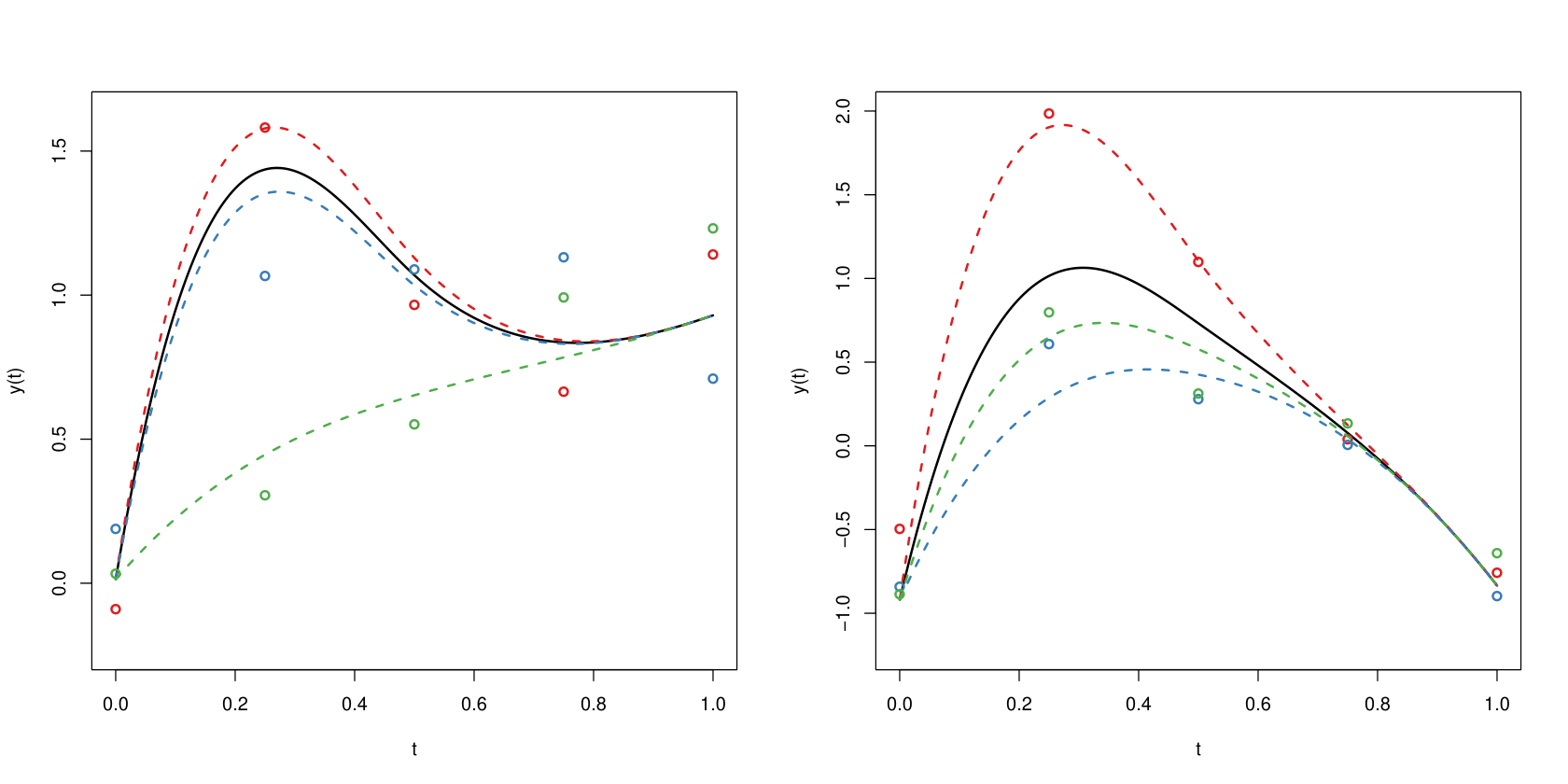
We discovered upon fitting the multi-level reduced-rank FPCA model with the normal assumption to real data that the fits were biologically implausible, an example of which is given on the left hand side of Figure 1. As can be clearly seen, the mean curve for this gene transcript, indicated by the solid line, does an unusually poor job of describing the underlying observations, being flat over the entire range of the time course. However, the replicate-level curves, indicated by the dashed lines, follow the observations much more closely. Upon further investigation, it became clear that this was due to an extreme departure from normality for the principal component loadings at the variable level, as can be seen in histograms of the initalised loadings for two example data sets given in Supplementary Figures 3 and 4, which exhibit heavy tails and varying degrees of skewness. To deal with this issue, we propose to instead adopt the assumption that the variable level loadings follow a skew-$t$-normal distribution, which is flexible enough to account for the heterogenous departures from normality. Formally, we assume that:

while retaining the assumption that $\bm{\beta}_{ij}$ and $\bm{\epsilon}_{ij}$ are multivariate normally distributed. $z\sim StN(\xi,\sigma^{2},\lambda,\nu)$ denotes that the random variable $z$ follows a skew-$t$-normal distribution (Gómez, Venegas and Bolfarine, 2007) where $\xi$ is a location parameter, $\sigma^{2}$ is a scale parameter, $\lambda$ is a skewness parameter and $\nu$ is the degrees of freedom controlling the kurtosis. The density of $z$ is given by

where $t_{\nu}(z;\xi,\sigma^{2})$ denotes the Student-t density with $\nu$ degrees of freedom, location parameter $\xi$ and scale parameter $\sigma^{2}$, and $\Phi$ denotes the normal cumulative distribution function. We note here in passing the closely related skew-t distribution of Azzalini and Capitanio (2003) which is identical in form to (4) except that the the normal cumulative distribution function, which controls the skewness of the density, is replaced by the Student-t cumulative distribution function, and depends not just on the skewness parameter $\lambda$ but also the degrees of freedom $\nu$. As Ho and Lin (2010) point out, evaluating the skew-t-normal density is therefore computationally simpler and the decoupling of the skewness from the degrees of freedom parameter is more conceptually sound.

Note that we have chosen not to use a multivariate skew-t-normal density for the variable-level loadings as this would require a single degrees of freedom parameter to be shared across all components, and we assume that they are independent anyway for the purposes of identifiability. Furthermore, we retain the original assumption that the replicate-level loadings follow a multivariate normal distribution. Judging from Figure 1, which is typical of other variables across multiple data sets, the replicate-level curves remain plausible under this assumption.

As in the Gaussian case, we can estimate the parameters under the assumptions given in (3) by treating the principal component loadings as missing data and employing the EM algorithm. The maximum likelihood estimators of $\bm{\theta}_{\mu}$, $\bm{\Theta}_{\alpha}$, $\bm{\Theta}_{\beta_{i}}$, $\bm{D}_{\beta_{i}}$ and $\sigma_{i}^{2}$ can be derived analytically as illustrated in the Supplementary Material. For the parameters of the skew-$t$-normal distributions, these can be estimated using Newton-Raphson (NR) as in Gómez, Venegas and Bolfarine (2007) or the EM algorithm as in Ho and Lin (2010). However, the NR approach relies on numerical integration and the EM algorithm is known to be slow to converge; alternatively, we have found that a simplex optimisation (Nelder and Mead, 1965) works very well in practice.

The conditional expectations that need to be calculated at the E-step of the EM algorithm based on these MLE estimators are summarised in Supplementary Table 2. However, expressions for these are challenging to obtain given that under the distributional assumptions, the marginal density of $\bm{y}_{i}$, as a sum of skew-t-normal and normal distributed random variables, follows no known form. In these circumstances we can instead turn to the Monte Carlo (MC) EM-algorithm (Wei and Tanner, 1990) which replaces the calculation of intractable expectations at the E-step with approximations based on averaging random samples drawn from the target density. As the target density is itself unknown, it is necessary to resort to stochastic simulation algorithms.

Given that the skew-$t$-normal distribution admits a convenient hierarchical representation, we suggest the use of the Gibbs sampler for drawing samples from the joint conditional distribution $f(\bm{\alpha}_{i},\bm{\beta}_{ij}|\bm{y}_{i})$. Specifically, following Ho and Lin (2010), if $\tau_{ik}\sim\Gamma(\nu_{\alpha_{k}}/2,\nu_{\alpha_{k}}/2)$ then

where $TN(\mu,\sigma^{2};(a,b))$ denotes the truncated normal distribution lying within the interval $(a,b)$. It can then be shown (see Supplementary Material) that

Therefore we introduce additional latent variables, $\bm{\tau}_{i}=[\tau_{i1}\cdots\tau_{iK}]^{T}$ and $\bm{\gamma}_{i}=[\gamma_{i1}\cdots\gamma_{iK}]^{T}$, and the target density for the Monte Carlo E-step becomes the joint conditional distribution $f(\bm{\alpha}_{i},\bm{\beta}_{i},\bm{\tau}_{i},\bm{\gamma}_{i}|\bm{y}_{i})$ whose form is still unknown. However, the conditionals $f(\bm{\alpha}_{i},\bm{\beta}_{i}|\bm{y}_{i},\bm{\tau}_{i},\bm{\gamma}_{i})$, $f(\bm{\tau}_{i}|\bm{y}_{i},\bm{\alpha}_{i},\bm{\beta}_{i},\bm{\gamma}_{i})$ and $f(\bm{\gamma}_{i}|\bm{y}_{i},\bm{\alpha}_{i},\bm{\beta}_{i},\bm{\tau}_{i})$ follow known distributions that are easy to sample from and hence the Gibbs sampler can be used to efficiently generate samples that are approximately distributed according to the target full joint conditional density.

Starting with $f(\bm{\alpha}_{i},\bm{\beta}_{i}|\bm{y}_{i},\bm{\tau}_{i},\bm{\gamma}_{i})$ note that from (5), conditional on $\tau_{ik}$ and $\gamma_{ik}$, $\alpha_{ik}$ is normally distributed with mean $\mu_{\alpha_{k}}=\xi_{\alpha_{k}}+\frac{\sigma_{\alpha_{k}}\lambda_{\alpha_{k}}}{\tau_{ik}+\lambda_{\alpha_{k}}^{2}}\gamma_{\alpha_{k}}$ and variance $v_{\alpha_{k}}=\frac{\sigma_{\alpha_{k}}^{2}}{\tau_{ik}+\lambda_{\alpha_{k}}^{2}}$. Hence we can write

where $\bm{\mu}_{\alpha}=[\mu_{\alpha_{1}}\cdots\mu_{\alpha_{K}}]^{T}$ and $\bm{v}_{\alpha}=[v_{\alpha_{1}}\cdots v_{\alpha_{K}}]^{T}$, $\bm{V}_{y_{i}|\tau_{i},\gamma_{i}}=\sigma^{2}_{i}\bm{I}_{N_{i}\times N_{i}}+\bm{B}_{i}\bm{\Theta}_{\alpha}\mbox{diag}(\bm{v}_{\alpha})\bm{\Theta}_{\alpha}^{T}\bm{B}_{i}^{T}+\widetilde{\bm{B}_{i}}\widetilde{\bm{\Theta}_{\beta_{i}}}\widetilde{\bm{D}_{\beta_{i}}}\widetilde{\bm{\Theta}_{\beta_{i}}^{T}}\widetilde{\bm{B}_{i}^{T}}$ and $\widetilde{\bm{D}_{\beta_{i}}}=\mbox{diag}(\bm{D}_{\beta_{i}},\cdots,\bm{D}_{\beta_{i}})$. Using a standard result from multivariate statistics (Anderson, 1958), we have that $f(\bm{\alpha}_{i},\bm{\beta}_{i}|\bm{y}_{i},\bm{\tau}_{i},\bm{\gamma}_{i})$ is therefore also multivariate normal (see Supplementary Material for specification of the mean and covariance), which is simple to sample from. For $f(\bm{\gamma}_{i}|\bm{y}_{i},\bm{\alpha}_{i},\bm{\beta}_{i},\bm{\tau}_{i})$ and $f(\tau_{i}|\bm{y}_{i},\bm{\alpha}_{i},\bm{\beta}_{i},\bm{\gamma}_{i})$, we use (6) and (7) respectively.

Having derived a process for calculating the required maximum likelihood estimators and conditional expectations, we are now in a position to summarise the complete MCEM algorithm for estimating the model parameters for the skew-$t$-normal multi-level reduced-rank FPCA model.

A procedure for initialisation is described in the Supplementary Material. After initialisation, the algorithm alternates between approximating the conditional expectations by running the Gibbs sampler for each variable at the E-step, and calculating the maximum likelihood estimators with their sufficient statistics replaced by the conditional expectations. Note that the maximum likelihood estimators of $\bm{\theta}_{\mu}$, and the individual columns of $\bm{\Theta}_{\alpha}$ and $\bm{\Theta}_{\beta_{i}}$ are interdependent. Therefore it is necessary to employ an Expectation Conditional Maximisation (ECM) algorithm where each part of the M-step is carried out holding all of the other parameters fixed. In other words, first $\bm{\theta}_{\mu}$ is estimated holding $\bm{\Theta}_{\alpha}$ and $\bm{\Theta}_{\beta_{i}}$ fixed. Next, the first column of $\bm{\Theta}_{\alpha}$ is estimated, holding all other columns of $\bm{\Theta}_{\alpha}$ fixed along with $\bm{\Theta}_{\beta_{i}}$ and $\bm{\theta}_{\mu}$, and so on. This process can be iterated as in James et al. (2000) or performed once per M-step as in Zhou et al. (2010). We have found the latter to work better in practice, in terms of numerical stability.

The maximum likelihood estimates of $\bm{\Theta}_{\alpha}$ and $\bm{\Theta}_{\beta_{i}}$ are not guaranteed to satisfy the constraint that the columns are orthogonal. While it is trivial to orthogonalise them by carrying out an eigen-decomposition, there is a lack of consensus as to whether this should be carried out at every iteration as in Zhou, Huang and Carroll (2008); Zhou et al. (2010) or once the EM algorithm has converged as in James et al. (2000). In the case of the former we sacrifice the monotonicity property of the EM algorithm in order to ensure that the estimates remain within the valid parameter space at each iteration. In the case of the latter the monotonicity property is retained but intuition suggests that the algorithm may converge to parameter values that are far from those which maximise the constrained likelihood once the orthogonalisation is carried out. In fact, in our experience with the model under the assumption of normality, orthogonalising at each iteration results in the algorithm converging to a marginally larger likelihood at the expense of many more iterations required before convergence, possibly due to some of the iterations decreasing the likelihood. Furthermore, we have found that when the full-rank model is fit, such that $K$ and $L_{i}$ are set to the maximum permitted by the choice of spline basis, computational instability can occur when orthogonalising at each iteration. An alternative to either of these approaches is to carry out the maximisation within the constrained parameter space - i.e. all matrices with orthonormal columns - as in Peng and Paul (2009). Such methods are difficult to implement due to their mathematical complexity and the success of James et al. (2000); Zhou, Huang and Carroll (2008); Zhou et al. (2010) suggest that, practically speaking, they are unnecessary.

The complete algorithm is as follows:

1. 1.

   Initialise parameters as described in the Supplementary Material

2. 2.

   E-step: For each variable, run the Gibbs sampler for $S$ iterations, sampling from $f(\bm{\alpha}_{i},\bm{\beta}_{i}|\bm{y}_{i},\bm{\tau}_{i},\bm{\gamma}_{i})$, $f(\bm{\tau}_{i}|\bm{y}_{i},\bm{\alpha}_{i},\bm{\beta}_{i},\bm{\gamma}_{i})$ and $f(\bm{\gamma}_{i}|\bm{y}_{i},\bm{\alpha}_{i},\bm{\beta}_{i},\bm{\tau}_{i})$ in turn

3. 3.

   M-step Step 1: Find the maximum likelihood estimators of the parameters of the skew-$t$-normal distributions using a simplex optimisation

4. 4.

   M-step Step 2: Update $\widehat{\bm{D}_{\beta_{i}}}$, $i=1,\cdots,M$

5. 5.

   M-step Step 3: Update $\widehat{\sigma_{i}^{2}}$, $i=1,\cdots,M$

6. 6.

   M-step Constrained Maximisation Step 1: Update $\widehat{\bm{\theta}}_{\mu}$ while holding $\widehat{\bm{\Theta}_{\alpha}}$ and $\widehat{\bm{\Theta}_{\beta_{i}}}$, $i=1,\cdots,M$ fixed

7. 7.

   M-step Constrained Maximisation Step 2: Update $\widehat{\bm{\Theta}_{\alpha}}$ while holding $\widehat{\bm{\theta}}_{\mu}$ and $\widehat{\bm{\Theta}_{\beta_{i}}}$, $i=1,\cdots,M$ fixed

8. 8.

   M-step Constrained Maximisation Step 3: Update $\widehat{\bm{\Theta}_{\beta_{i}}}$, $i=1,\cdots,M$ while holding $\widehat{\bm{\theta}}_{\mu}$ and $\widehat{\bm{\Theta}_{\alpha}}$ fixed

9. 9.

   Check for convergence. If not converged, return to 3.

10. 10.

    Orthogonalise $\widehat{\bm{\Theta}_{\alpha}}$ and $\widehat{\bm{\Theta}_{\beta_{i}}}$, $i=1,\cdots,M$

Two remaining issues are how to select the number of principal components, both at the variable- and replicate-level, and what spline basis to use. For selecting the number of principal components, two main approaches can be considered. In the first, the proportion of variance explained by each principal component function can be approximated by fitting the full-rank model - such that $K$ and $L_{i}$ (for all $i$) are the maximum permitted by the number of design time points (James et al., 2000). For the second method, cross-validation is used to score each potential value of $K$ and $L_{i}$ (Zhou et al., 2010). Note that both of these approaches require a subjective interpretation. For the proportion of variance explained method, either an arbitrary cutoff for cumulative variance such as $95\%$ or $99\%$ must be used, perhaps aided by an examination of a scree plot and a visualisation of the principal component functions in order to ascertain their interpretability. On the other hand, as Zhou et al. (2010) discuss, when using the cross-validation method on real data the score may simply decrease as the number of principal components increases, which results in always selecting the full-rank model going by the score alone. Therefore they suggest to instead subjectively trade-off between parsimony and cross-validation score, again with the aid of a scree plot. However, in the model of Zhou et al. (2010), the number of principal components at the second-level is not dependent on the first-level and so the cross-validation method is much more tractable in their setting than ours, where the high-dimensional optimisation renders the approach impractical. By necessity therefore, we employ the proportion of variance explained method. On simulated data we have discovered that this works very well at identifying the correct number of principal components at the variable-level, but struggles at the replicate-level, most likely due to the much smaller sample sizes. We therefore suggest that a (much) more conservative criteria be applied at the replicate-level. For instance, we have found that retaining those principal components that explain $99\%$ of the variance at the variable-level and $60\%$ of the variance at the replicate-level worked well on these data sets.

For selecting the spline basis we suggest to use natural cubic splines with a knot placed at each design time point for several reasons. Firstly, this avoids the computational burden of having to select the number of knots. Secondly, many of the data sets provided by our collaborators have unequally spaced time points, and it therefore makes sense to use each time point as a knot in order to adequately capture the temporal dynamics. Thirdly, the reason to countenance against such an approach would be the danger of overfitting. This is accounted for through the use of the reduced-rank model, essentially placing a rank-constraint on the covariance matrix of the spline basis coefficients. Conceptually speaking, this approach to spline basis selection is quite similar to the use of smoothing splines, where a knot is placed at each design time point and overfitting is avoided through the use of a penalty parameter on the likelihood.

We set out to determine whether single-level approaches that assume the variables are independent are adequate when it comes to estimating the true underlying curves, and to quantify the improvement that can be gained through the use of a multi-level model using the following simulation setting.

We generated data under the multi-level reduced-rank FPCA model (2) with normality assumed, as the skew-$t$-normal model is too computationally intensive, with its reliance on MC methods, for large scale simulation studies. We fixed the number of principal components at the variable level to $K=2$ with a single principal component at the replicate level for each variable, so that $L_{i}=1$ for all $i$. We used a B-spline basis with a single knot placed at the centre of the time course. The spline coefficients for the grand mean, $\bm{\theta}_{\mu}$, were fixed to produce the curve that can be seen in Figure 3.

The spline coefficients for the variable-level principal component functions, $\bm{\theta}_{\alpha_{1}}$ and $\bm{\theta}_{\alpha_{2}}$ were chosen in order to produce the simulated curves given in Figure 2. Visualising the grand mean plus and minus each principal component function is a typical way of helping to understand their effect (Ramsay and Silverman, 2005). These plots are given in Figure 3. The solid line is the grand mean. The points denoted by ‘$+$’ are the function $\mu(t)+C\zeta_{k}(t)$ evaluated on a coarse grid of points where $C$ is some constant responsible for scaling the principal component function and subjectively chosen in order to aid clarity of the visualisation. Similarly, the points denoted by ‘$-$’ are the same except for $\mu(t)-C\zeta_{k}(t)$. From these plots it should be clear that the first principal component has the effect of rotating the first half of the time course, which alters both the level at which the time course begins and the level to which it peaks. To a lesser extent the exact time at which the peak occurs is also affected. On the other hand, the second principal component function rotates the second half of the time course, thereby controlling whether the curve levels off, continues to decrease or starts to increase after the peak and the dip.

For the replicate-level principal components, the same principal component function was fixed for all variables. Note that this only serves to simplify the simulation scheme, and the multi-level reduced-rank FPCA model will still estimate the between-replicate variation for each variable independently. By choosing the spline coefficients $\bm{\theta}_{\beta_{1}}$ to produce the profile given on the left hand side of Figure 4, the effect of the principal component function is to scale the height to which the curves peak, as shown on the right hand side of the same Figure.

The remaining parameters to be determined are the variance components $\bm{D}_{\alpha}$, $\bm{D}_{\beta_{i}}$ and $\sigma_{i}^{2}$ for all $i$. We set $\bm{D}_{\alpha}=\mbox{diag}(0.3,0.1)$ so that $75\%$ of the variance at the variable level is explained by the first principal component function. The single element of $\bm{D}_{\beta_{i}}$ was set to $0.075$ for all $i$ so that the level of between-replicate variance is less than that of the between-variable. Similarly, the noise was set to $\sigma_{i}^{2}=0.05$ for all $i$. As before, this only serves to simplify the simulation scheme and separate estimates will be made for $\bm{D}_{\beta_{i}}$ and $\sigma_{i}^{2}$ for each variable. The simulation scheme described here is flexible enough to produce a wide range of believable curves as evidenced by the examples given in Supplementary Figure 5.

In order to compare the single- and multi-level reduced-rank FPCA models under a range of experimental designs and to determine whether standard practice is appropriate, we generated different data sets by varying the number of replicates as either $5$, $10$ or $20$. Roughly speaking, with regards real data sets, these correspond to realistic, less frequent and unrealistic numbers of replicates respectively. The number of time points per data set was fixed to $5$. We focused on evaluating the ability to estimate the variable-level curves and for this reason we also varied the number of variables between $100$, $1,000$ and $10,000$. Although broadly speaking $10,000$ is the only realistic value of the three for ‘omics data sets (unless the variables have been subject to some initial filtering procedure), we were interested in exploring the properties of the multi-level model and determining how many variables are required to adequately assess the between-variable variation.

We generated $1,000$ data sets under each condition. For each data set we fit both the single- and multi-level reduced-rank FPCA models under the assumption of normality. For the purposes of this study we chose not to consider the issue of correctly selecting the number of principal component functions at the variable- and replicate-levels and the number or location of the knots of the spline basis and simply input the correct values to each algorithm. We compared each variable-level curve by discretising it on a fine grid of points and calculating the mean squared error between it and the underlying true curve. We then averaged this error across all variables and all data sets to give a single measure for each model for each condition.

The complete results of the simulation study are presented in Supplementary Tables 3 and 4. In all scenarios the multi-level model substantially improves upon the single-level model. For the multi-level model, doubling the number of replicates roughly halves the estimation error. However, increasing the number of variables has a much less pronounced effect, suggesting the multi-level model still performs well when data sets have been pre-filtered. For the single-level model, doubling the number of replicates similarly roughly halves the estimation error. As expected, increasing the number of variables for this model has no effect on the estimation error as each variable is fit in isolation. The most salient insight to glean from these results is in the comparison between the two tables. Comparing first the case of $5$ replicates and $10,000$ variables for the two models, the multi-level model offers an improvement in estimation error of approximately a factor of ten. Considering the single-level model alone, in order to attain an equivalent improvement in estimation error, the number of replicates needs to quadruple from $5$ to $20$. These results suggest that simply using a more sophisticated model has the potential to dramatically reduce experimental costs.

We fit the skew-$t$-normal multi-level reduced-rank FPCA model to a genomics data set study the genetic response to infection by BCG, the vaccine for tuberculosis, in $9$ human volunteers. We determined that the MCEM algorithm had converged after $1050$ iterations by examining parameter trace plots. On the right hand side of Figure 1 we show the fit obtained under the new model to the CCL20 transcript. As can be clearly seen, the mean curve is much more reasonable, closely following the underlying observations.

The variable-level principal component functions are given in Figure 5. The first principal component – which explains a huge proportion of the variance, $99.998\%$ – is responsible for vertically shifting a given transcript. In this respect, it is the most uninteresting of the principal component functions as it does not control the shape of the curves. We stress that it is not suprising that such a large proportion of the variance is explained by vertical shifts given that very few of the tens of thousands of variables in an ‘omics data set will actually exhibit significant changes over time. It is therefore still instructive to consider the other principal component functions even if the proportion of variance they explain may lead to them being overlooked in more traditional PCA application areas.

The second principal component function accounts for those transcripts which rapidly spike before plateauing at some elevated level of expression or, conversely, are rapidly repressed. The CCL20 transcript is a example of this. The third principal component function describes those transcripts which are induced or repressed more slowly, tailing off at around $7$ or $8$ hours. In Supplementary Figure 6 we give an example of a transcript that exhibits this profile and was found to have the highest positive loading on the third principal component function. More complex profiles can be explained by a combination of these two components. The fourth principal component function is less interpretable but appears to be mainly controlling for variation at the end of the time course. The fifth principal component function is even less interpretable and should probably be discarded when the data is fit for a second time under the reduced-rank model.

References

- Anderson (1958) [author] Anderson, Theodore W.T. W. (1958). Introduction to Multivariate Statistical Analysis. Wiley. \endbibitem
- Angelini, Canditiis and Pensky (2009) [author] Angelini, ClaudiaC., Canditiis, Daniela DeD. D. and Pensky, MariannaM. (2009). Bayesian models for two-sample time-course microarray experiments. Computational Statistics & Data Analysis 53 1547 - 1565. Statistical Genetics & Statistical Genomics: Where Biology, Epistemology, Statistics, and Computation Collide. \endbibitem
- Azzalini and Capitanio (2003) [author] Azzalini, A.A. and Capitanio, A.A. (2003). Distributions generated by perturbation of symmetry with emphasis on a multivariate skew-t distribution. Journal of the Royal Statistical Society, Series B 65 367-389. \endbibitem
- Berk, Ebbels and Montana (2011) [author] Berk, M.M., Ebbels, T.T. and Montana, G.G. (2011). A statistical framework for metabolic profiling using longitudinal data. Bioinformatics 27 1979 - 1985. \endbibitem
- Berk et al. (2010) {binproceedings}[author] Berk, M.M., Montana, G.G., Levin, M.M. and Hemingway, C.C. (2010). Longitudinal analysis of gene expression profiles using functional mixed-effects models. In Studies in Theoretical and Applied Statistics. \endbibitem
- Di et al. (2009) [author] Di, C.C., Crainiceanu, C. M.C. M., Kuechenhoff, H.H. and Peters, A.A. (2009). Multilevel functional principal component analysis. Annals of Applied Statistics 3 458 - 488. \endbibitem
- Forchini (2008) [author] Forchini, G.G. (2008). The distribution of the sum of a normal and a t random variable with arbitrary degrees of freedom. METRON - International Journal of Statistics 2 205-208. \endbibitem
- Gómez, Venegas and Bolfarine (2007) [author] Gómez, Hector W.H. W., Venegas, OsvaldoO. and Bolfarine, HelenoH. (2007). Skew-symmetric distributions generated by the distribution function of the normal distribution. Environmetrics 18 395–407. \endbibitem
- Ho and Lin (2010) [author] Ho, Hsiu J.H. J. and Lin, Tsung-I.T.-I. (2010). Robust linear mixed models using the skew t distribution with application to schizophrenia data. Biometrical Journal 52 449 - 469. \endbibitem
- James, Hastie and Sugar (2000) [author] James, GMG., Hastie, TJT. and Sugar, CAC. (2000). Principal component models for sparse functional data. Biometrika 87 587-602. \endbibitem
- Jara, Quintana and Martin (2008) [author] Jara, AlejandroA., Quintana, FernandoF. and Martin, Ernesto SanE. S. (2008). Linear mixed models with skew-elliptical distributions: A Bayesian approach. Computational Statistics & Data Analysis 52 5033 - 5045. \endbibitem
- Liu and Yang (2009) [author] Liu, XueliX. and Yang, Mark C. K.M. C. K. (2009). Identifying temporally differentially expressed genes through functional principal components analysis. Biostat kxp022. \endbibitem
- Ma et al. (2006) [author] Ma, PingP., Castillo-Davis, Cristian IC. I., Zhong, WenxuanW. and Liu, Jun SJ. S. (2006). A data-driven clustering method for time course gene expression data. Nucleic Acids Res 34 1261–1269. \endbibitem
- Montana, Berk and Ebbels (2011) [author] Montana, G.G., Berk, M.M. and Ebbels, T.T. (2011). Software Tools and Algorithms for Biological Systems Modelling short time series in metabolomics: a functional data analysis approach 307-316. Springer, New York. \endbibitem
- Nelder and Mead (1965) [author] Nelder, J. A.J. A. and Mead, R.R. (1965). A Simplex Method for Function Minimization. The Computer Journal 7 308-313. \endbibitem
- Peng and Paul (2009) [author] Peng, JieJ. and Paul, DebashisD. (2009). A Geometric Approach to Maximum Likelihood Estimation of the Functional Principal Components From Sparse Longitudinal Data. Journal of Computational and Graphical Statistics 18 995-1015. \endbibitem
- Ramsay and Silverman (2005) [author] Ramsay, JimJ. and Silverman, B. W.B. W. (2005). Functional Data Analysis, 2 ed. Springer, New York. \endbibitem
- Storey et al. (2005) [author] Storey, John DJ. D., Xiao, WenzhongW., Leek, Jeffrey TJ. T., Tompkins, Ronald GR. G. and Davis, Ronald WR. W. (2005). Significance analysis of time course microarray experiments. Proc Natl Acad Sci U S A 102 12837–12842. \endbibitem
- Tai and Speed (2009) [author] Tai, Yu ChuanY. C. and Speed, Terence P.T. P. (2009). On Gene Ranking Using Replicated Microarray Time Course Data. Biometrics 65 40-51. \endbibitem
- Tusher, Tibshirani and Chu (2001) [author] Tusher, Virginia GossV. G., Tibshirani, RobertR. and Chu, GilbertG. (2001). Significance analysis of microarrays applied to the ionizing radiation response. Proceedings of the National Academy of Sciences of the United States of America 98 5116-5121. \endbibitem
- Wei and Tanner (1990) [author] Wei, Greg C. G.G. C. G. and Tanner, Martin A.M. A. (1990). A Monte Carlo Implementation of the EM Algorithm and the Poor Man’s Data Augmentation Algorithms. Journal of the American Statistical Association 85 pp. 699-704. \endbibitem
- Yao, Müller and Wang (2005) [author] Yao, FangF., Müller, Hans-GeorgH.-G. and Wang, Jane-LingJ.-L. (2005). Functional Data Analysis for Sparse Longitudinal Data. Journal of the American Statistical Association 100 577-590. \endbibitem
- Zhou, Huang and Carroll (2008) [author] Zhou, LanL., Huang, Jianhua Z.J. Z. and Carroll, Raymond J.R. J. (2008). Joint modelling of paired sparse functional data using principal components. Biometrika 95 601-619. \endbibitem
- Zhou et al. (2010) [author] Zhou, LanL., Huang, Jianhua Z.J. Z., Martinez, Josue G.J. G., Maity, ArnabA., Baladandayuthapani, VeerabhadranV. and Carroll, Raymond J.R. J. (2010). Reduced Rank Mixed Effects Models for Spatially Correlated Hierarchical Functional Data. Journal of the American Statistical Association 105 390-400. \endbibitem
Supplementary Material for “A Skew--Normal Multi-Level Reduced-Rank Functional PCA Model with Applications to Replicated ‘Omics Time Series Data Sets”
1 The Gaussian multi-level reduced-rank FPCA model
For the Gaussian case we take the following distributional assumptions:
- Anderson (1958) T. W. Anderson. Introduction to Multivariate Statistical Analysis. Wiley, 1958.
- James et al. (2000) G. James, T. Hastie, and C. Sugar. Principal component models for sparse functional data. Biometrika, 87(3):587–602, 2000.
- Peng and Paul (2009) J. Peng and D. Paul. A geometric approach to maximum likelihood estimation of the functional principal components from sparse longitudinal data. Journal of Computational and Graphical Statistics, 18(4):995–1015, 2009.
- Zhou et al. (2010) L. Zhou, J. Z. Huang, J. G. Martinez, A. Maity, V. Baladandayuthapani, and R. J. Carroll. Reduced rank mixed effects models for spatially correlated hierarchical functional data. Journal of the American Statistical Association, 105(489):390–400, 2010.