Linear Correction of Mismatched L-values
in BICM receiversThanks: The work was supported by the government of Quebec, under grant #PSR-SIIRI-435. Parts of this work have been submitted to IEEE International Conference on Communications 2012.

The logarithmic likelihood ratios (LLRs, or L-values) calculated at the receiver for the transmitted bits, are a convenient representation of the likelihood of the observations and are often used in all of the processing operations in the receiver (such as “soft” detection, decoding, iterative processing, etc). In this work we consider the so-called mismatched L-values, which only approximate the true L-values and to “correct” the mismatch, that may occur due to many independent reasons, we analyze the linear scaling of the mismatched L-values. Formulating the problem in the context of BICM receivers, we aim at the minimization of the probability of error of the maximum likelihood (ML) decoder that uses the corrected L-values.

The L-value $l_{n}$ of the bit $C_{n}$ (transmitted at time $n$) is a well known way of representing the reliability of the transmitted bit. It is related to the observation $y_{n}$ via

where $p_{Y_{n}|C_{n}}(y_{n}|b)$ is the probability density function (pdf) of the observation $Y_{n}$ conditioned on the sent bit $C_{n}=b$.

The L-values are basic signals/messages exchanged between the processing units. The multiplications of probabilities required in many processing steps transform into addition of corresponding L-values; the numerical simplicity of the resulting operations is the reason behind the popularity of the L-values. For example, in BICM receivers, the L-values are calculated by the front-end detector and then passed to the decoder [1]. In some cases, operations on the L-values are carried out before decoding as it happens when combining the signals obtained in independent transmissions of the same bit [2]. The L-values are also used in binary decoders that operate in an iterative fashion, e.g., turbo-decoders [3] or message passing algorithms used for decoding of LDPC codes [4].

In some situations, however, the L-values are not appropriately calculated, or are mismatched. Ignoring the mismatch when processing the L-values is, in general, suboptimal and to correct it, nonlinear operations on the L-values may be required. To make the correction simple, a linear operation (i.e., multiplication by a correction factor) is often considered. This idea was already studied in the context of BICM receivers [5], turbo-decoding [6][7], or LDPC decoding [4]. However, the correction factor was most often found through a brute-force search, that is, among the results obtained for different correction factors the one ensuring the best performance is deemed optimal. While this is a pragmatic approach when searching for one or two correction factors, it cannot be applied when many correction factors have to be found (the search space becomes too large) and/or when the correction has to be done on-line (i.e., when it depends on many continuously varying parameters).

The works in [6][8][9][10][11] aimed at finding the correction factor using the pdf of the L-value. The method of [6], based on a Gaussian model of the L-value fails to capture properties of non-Gaussian pdfs while [8] draws general conclusions about the suitability of linear correction but relies on simulation to find the correction factor. [9][10][11] rely on the minimization of a functional of the pdf which requires numerical integration as in most cases the analytical solutions are not available. The drawbacks of [9] is that the pdf has to be known or estimated and the functional in the optimization problem is not related to any performance criterion. This disadvantages were recently removed in [10][11], where the correction factor was formally found via maximization of the so-called generalized mutual information (GMI) between the L-values and the corresponding bits. Then, even if the pdf is not known, the Monte-Carlo integration can be implemented. While this approach was (experimentally) shown to improve the performance of BICM receivers operating with the capacity-approaching codes, it does not explicitly address the problem of minimizing the error probability of the optimal maximum-likelihood (ML) decoder.

In this paper we explicitly aim at the minimization of the probability of error in ML decoders, which results in a novel correction principle and provides a new insight into correction of the L-values. Our problem is formulated in the domain of the cumulative generating function (CGF) of the L-values. As their calculation is simpler than finding the pdf, in many cases we will be able to avoid explicit numerical integration. We find a simple correction principle which says that the correction factor should be equal to the twice of the so-called saddlepoint of the CGF, which is the real argument minimizing the CGF. Finding the saddlepoint requires solving a simple non-linear equation which, in many cases, may be even found analytically.

The paper is organized as follows. The definitions and notation are presented in Sec. II and the new correction principle we propose is explained in Sec. III. A detailed illustration of our analysis in shown in Sec. IV on an example of correction of the L-values in the BICM receivers operating in the presence of interference.

We consider a scenario where a codeword of $N$ bits $\boldsymbol{c}=[c_{1},c_{2},\ldots,c_{N}]$ is sent over a binary-input memoryless channel with known transition probability given by the pdf $p_{Y_{n}|C_{n}}(y_{n}|c_{n})$.

Upon reception of $y_{1},\ldots,y_{N}$, in order to minimize the probability of detection error, the decoder decides in favour of the codeword that maximizes the likelihood of the observation, i.e.,

where $\mathcal{C}$ is the code (i.e., set of all codewords).

Using Bayes’ formula $p_{Y_{n}|C_{n}}(y_{n}|c_{n})=P_{C_{n}|Y_{n}}(c_{n}|y_{n})p_{Y_{n}}(y_{n})/P_{C_{n}}(c_{n})$ in (1), and knowing that $P_{C_{n}|Y_{n}}(c_{n}|y_{n})=1-P_{C_{n}|Y_{n}}(1-c_{n}|y_{n})$, we obtain a useful alternative expression of the aposteriori probabability $P_{C_{n}|Y_{n}}(c_{n}|y_{n})=e^{l_{n}\cdot c_{n}}/(1+e^{l_{n}})$. It transforms (2) into the decoding based on the L-values

where the terms independent of $\boldsymbol{c}$ were removed from the maximization in (3).

The L-values $l_{n}$ are modelled as random variables $L_{n}$ and if they are calculated exactly as defined in (1) their pdf satisfies the so-called consistency condition [12, Sec. III]

The so-called symmetry condition [12, Sec. III]

simplifies the analysis and, although it does not have to be always satisfied (it depends on the conditional pdf $p_{Y_{n}|C_{n}}(y_{n}|c_{n})$), it may be forced by a pseudo-random scrambling of the bits $c_{n}$ prior to modulation, followed by the change of the sign of the L-values $l_{n}$ if the bit was negated [13]. Thus, from now on, we assume that this condition is always satisfied.

Rewriting (4) as $p_{L_{n}|C_{n}}(l|1)\textrm{e}^{-l/2}=\textrm{e}^{l/2}p_{L_{n}|C_{n}}(l|0)$ and using (5) yields what we call a consistency-symmetry condition

Now, we want answer the question: how to choose the correction factors $\{\alpha_{n}\}_{n=1}^{N}$ so that the error of the decoder that uses the corrected L-values $\tilde{l}^{\textrm{c}}_{n}=\alpha_{n}\cdot\tilde{l}_{n}$ is minimized?

From the previous discussion we conclude that, in order to improve the performance of the decoder, we should find $\{\alpha_{n}\}_{n=1}^{N}$ to minimizes the $\textrm{PEP}\left(\{\alpha_{n}\}_{n=1}^{N},\hat{\boldsymbol{c}}\right)$ in (18) for any codeword $\hat{\boldsymbol{c}}$. Thus, we have to solve the following optimization problem

and its solution should be independent of $\hat{\boldsymbol{c}}$ because we want to apply the correction factors to all L-values prior to decoding and we do not know which error ($\boldsymbol{c}\rightarrow\hat{\boldsymbol{c}}$) will occur.

At first sight, the problem may appear intractable due to the dependance of the PEP on various $\hat{\boldsymbol{c}}$, each resulting in a different set of L-values indexed by $\{n_{k}\}_{k=1}^{d}$ which are then convolved as per (19).

Consider a BPSK transmission, when the sent symbols $x_{n}=2c_{n}-1$ pass through a channel affected by additive Gaussian noise and a BPSK interference

where $h_{n}\in\mathcal{R}$ is the known gain of the channel, $z_{n}$ is a zero-mean Gaussian signal with known variance $\sigma_{z}^{2}=N_{0}/2$; $d_{n}\in\{-1,1\}$ is the BPSK-modulated interference signal received with the gain $g_{n}\in\mathcal{R}$. We define also the SNR and the signal-to-interference ratio (SIR), respectively, as $SNR=h_{n}^{2}/N_{0}$ and $SIR=h_{n}^{2}/g_{n}^{2}$.

Although using (1) it is relatively simple to calculate the L-values in this case as

for the purpose of our examples, the receiver ignores the interference, thus assumes $g_{n}=0$, and then, from (44) we obtain the L-value

which is mismatched due to assumed absence of interference.

To apply the correction principle we derived, we need to calculate the CGF of $\tilde{L}=\frac{2h_{n}}{\sigma_{z}^{2}}\cdot Y$, conditionned on sending the bit $c_{n}=0$, $\kappa_{\tilde{L}}(s)=\kappa_{Y}(\frac{2h_{n}}{\sigma_{z}^{2}}s)$, where

Then, finding the saddlepoint of $\kappa_{Y}(s)$, as $\kappa_{Y}^{\prime}(\hat{s})=0$, the saddlepoint of $\kappa_{\tilde{L}}(s)$ equals to $\frac{\sigma^{2}_{z}}{2h_{n}}\hat{s}$ thus, the correction factor applied to the $\tilde{l}_{n}$ is given by (37) $\hat{\alpha}=\frac{\sigma_{z}^{2}}{h_{n}}\hat{s}$ and the correction boils down to the calculation

Note that, instead of calculating the saddlepoint of $\kappa_{\tilde{L}}(s)$ and correcting $\tilde{l}_{n}$, we might directly calculate the saddlepoint of $\kappa_{Y}(s)$ and apply it to the observation $y_{n}$. This is possible, of course, because the L-value $\tilde{l}_{n}$ is a scaled version of $y_{n}$, cf. (45).

To find the saddlepoint $\hat{s}$ we differentiate (46) to obtain the following saddlepoint equation

whose graphical interpretation as the intersection of the right-had- and left-hand sides is shown in Fig. 1.

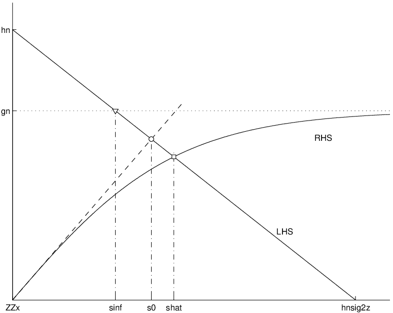
While (48) cannot be solved in a closed-form, we may obtain approximations in particular cases. Namely, for $SNR\rightarrow 0$ (i.e., when $\sigma_{z}^{2}\rightarrow\infty)$, we easily see that $\hat{s}\rightarrow 0$ so, using the linearization $\tanh(x)\approx x$ (shown as a dashed line in Fig. 1), we obtain

where $\sigma_{\textrm{N+I},n}^{2}$ is the variance of the noise and interference. The corresponding correction factor is given by $\alpha^{0}=\frac{\sigma_{z}^{2}}{\sigma_{\textrm{N+I},n}^{2}}$. Note that using $\tilde{\mu}=-\mathds{E}_{\tilde{L}_{n}|C_{n}=0}=\frac{h^{2}_{n}}{\sigma^{2}_{z}}$ and $\tilde{\sigma}^{2}=\textrm{Var}\{\tilde{L}_{n}\}=\frac{4h^{2}_{n}}{\sigma^{4}_{z}}$ in (10) yields exactly the same results $\alpha^{\textrm{Gauss}}=\alpha^{0}$.

This means that for the low SNR, when the noise “dominates” the interference, the effect of noise and the interference can be modelled as a Gaussian variable with variance $\sigma_{\textrm{N+I},n}^{2}$; this is often done in practice [21] and the corrected L-values, in this case, would be calculated as

For high SNR, i.e., when $SNR\rightarrow\infty$ (i.e., $\sigma_{z}^{2}\rightarrow 0$), we observe that $\hat{s}\rightarrow-\infty$ so taking advantage in (48) of the saturation of $\tanh(\infty)=1$, the saddlepoint is given by¹¹ 1 We assume $g_{n}<h_{n}$, i.e., the interference is weaker than the desired signal.

and the corresponding correction factor by

The L-values in this case would be calculated as

that is, the interference-related term decreases the gain of the useful signal. Intuitively, this can be explained as follows: for high SNR, the interference can be “distinguished” from the noise and becomes the part of the transmitted constellation, i.e., sending bit $c_{n}=1$, we will effectively be able to make a difference between $h_{n}-g_{n}$ or $h_{n}+g_{n}$. Moreover, for high SNR the symbol that is the most likely to provoke the error is the one closest to the origin, that is $h_{n}-g_{n}$. This leads to assuming that BPSK symbols are sent over a channel with gain $h_{n}-g_{n}$, cf. (53).

For $0<SNR<\infty$, the saddlepoint can be obtained numerically solving (48). For example, we might use the Newton-Raphson method

where

and $\hat{s}(0)$ is the appropriately chosen starting point for the recursion, e.g., $\hat{s}(0)=\max\{\hat{s}^{\infty},\hat{s}^{0}\}$. In this work, we used $I_{\textrm{max}}=2$ so a small computation load in incurred due to the on-line calculation of the the correction factors; alternatively, the correction factors might be interpolated using a table precalculated for different values of $SNR$ and $SIR$.

Since $\frac{h_{n}}{\sigma_{z}^{2}}>\hat{s}$ (cf. Fig. 1) we can also immediately conclude that the correction factor always satisfies $\hat{\alpha}=\frac{\sigma_{z}^{2}}{h_{n}}\hat{s}<1$, that is, ignoring the interference, our reliability metric is too “optimistic” and must be scaled down. On the other hand, since $\hat{s}>\hat{s}^{0}$, if the mismatched L-value is calculated using the Gaussian approximation of the interference, that is using (50), the correction would be $\hat{\alpha}>1$. That is, the Gaussian approximation is too “pessimistic”.

We show in Fig. 2 the values of the optimal correction factors for different values of SNR and SIR. For high SNR, as predicted by (52), $\hat{\alpha}=\hat{\alpha}^{\infty}=1-g_{n}=1-10^{-SIR/20}$; for example, when $SIR=6$ dB, $\hat{\alpha}=0.5$. We also show the value of $\hat{\alpha}^{\textrm{GMI}}$, cf. (12) and we see that it is quite close to $\hat{\alpha}$. Both factors are increasing with SINR as the case $SINR\rightarrow\infty$ corresponds to the assumed absence of the interference, that is, $\hat{\alpha}\rightarrow 1$.

References

- [1] E. Zehavi, “8-PSK trellis codes for a Rayleigh channel,” IEEE Trans. Commun., vol. 40, no. 3, pp. 873–884, May 1992.
- [2] C. Wengerter, A. von Elbwart, E. Seidel, G. Velev, and M. Schmitt, “Advanced hybrid ARQ technique employing a signal constellation rearrangement,” in IEEE Vehicular Technology Conference 2002, VTC-2002 Fall, Sep. 2002, pp. 2002–2006.
- [3] S. Benedetto, D. Divsalar, G. Montorsi, and F. Pollara, “A soft-input soft-output APP module for iterative decoding of concatenated codes,” IEEE Commun. Lett., vol. 1, no. 1, pp. 22–24, Jan. 1997.
- [4] J. Chen and M. Fossorier, “Near optimum universasl belief propagation based decoding of low-density parity check codes,” IEEE Trans. Commun., vol. 50, no. 3, pp. 406–414, 2002.
- [5] B. Classon, K. Blankenship, and V. Desai, “Channel coding for 4G systems with adaptive modulation and coding,” IEEE Wireless Commun. Mag., vol. 9, no. 2, pp. 8–13, Apr. 2002.
- [6] L. Papke, P. Robertson, and E. Villebrun, “Improved decoding with the SOVA in a parallel concatenated (turbo-code) scheme,” in International Conference on Communications, ICC 96, vol. 1, Jun 1996, pp. 102–106.
- [7] J. Vogt and A. Finger, “Improving the max-log-map turbo decoder,” IEEE Electronic Letters, vol. 36, no. 23, pp. 1937–1939, Nov. 2000.
- [8] M. van Dijk, A. Janssen, and A. Koppelaar, “Correcting systematic mismatches in computed log-likelihood ratios,” Eur. Trans. on Telecommun., vol. 14, no. 3, pp. 227–224, 2003.
- [9] G. Lechner and J. Sayir, “Improved sum-min decoding for irregular LDPC codes,” in International Symposium on Turbo Codes & Related Topics, Apr. 2006.
- [10] T. Nguyen and L. Lampe, “Bit-interleaved coded modulation with mismatched decoding metrics,” IEEE Trans. Commun., vol. 59, no. 2, pp. 437–447, Feb. 2011.
- [11] R. Yazdani and M. Ardakani, “Efficient LLR calculation for non-binary modulations over fading channels,” IEEE Trans. Commun., vol. 59, no. 5, pp. 1236 –1241, May 2011.
- [12] M. Tüchler, “Design of serially concatenated systems depending on the block length,” IEEE Trans. Commun., vol. 52, no. 2, pp. 209–218, Feb. 2004.
- [13] G. Caire, G. Taricco, and E. Biglieri, “Bit-interleaved coded modulation,” IEEE Trans. Inf. Theory, vol. 44, no. 3, pp. 927–946, May 1998.
- [14] A. Martinez, A. Guillén i Fàbregas, and G. Caire, “Bit-interleaved coded modulation revisited: A mismatched decoding perspective,” IEEE Trans. Inf. Theory, vol. 55, no. 6, pp. 2756–2765, Jun. 2009.
- [15] A. Alvarado, V. Núñez, L. Szczecinski, and E. Agrell, “Correcting suboptimal metrics in iterative decoders,” in IEEE International Conference on Communications, ICC 2009, Dresden, Germany, Jun. 2009.
- [16] G. Lechner, “Efficient decoding techniques for LDPC codes,” Ph.D. dissertation, Vienna University of Technology, Austria, Jul. 2007.
- [17] A. Martinez, A. Guillén i Fàbregas, and G. Caire, “A closed-form approximation for the error probability of BPSK fading channels,” IEEE Trans. Wireless Commun., vol. 6, no. 6, pp. 2051–2054, Jun. 2007.
- [18] ——, “Error probability analysis of bit-interleaved coded modulation,” IEEE Trans. Inf. Theory, vol. 52, no. 1, pp. 262–271, Jan. 2006.
- [19] L. Szczecinski, A. Alvarado, and R. Feick, “Distribution of max-log metrics for QAM-based BICM in fading channels,” IEEE Trans. Commun., vol. 57, no. 9, pp. 2558–2563, Sep. 2009.
- [20] A. Kenarsari-Anhari and L. Lampe, “An analytical approach for performance evaluation of BICM transmission over Nakagami-m fading channels,” IEEE Trans. Commun., vol. 58, no. 4, pp. 1090 –1101, april 2010.
- [21] M. Sellathurai and S. Haykin, “Turbo-BLAST for wireless communications: theory and experiments,” IEEE Trans. Signal Process., vol. 50, no. 10, pp. 2538 –2546, Oct. 2002.
- [22] P. Frenger, P. Orten, and T. Ottosson, “Convolutional codes with optimum distance spectrum,” IEEE Trans. Commun., vol. 3, no. 11, pp. 317–319, Nov. 1999.