An Optimal Controller Architecture for Poset-Causal Systems
Abstract
We propose a novel and natural architecture for decentralized control that is applicable whenever the underlying system has the structure of a partially ordered set (poset). This controller architecture is based on the concept of Möbius inversion for posets, and enjoys simple and appealing separation properties, since the closed-loop dynamics can be analyzed in terms of decoupled subsystems. The controller structure provides rich and interesting connections between concepts from order theory such as Möbius inversion and control-theoretic concepts such as state prediction, correction, and separability. In addition, using our earlier results on -optimal decentralized control for arbitrary posets, we prove that the -optimal controller in fact possesses the proposed structure, thereby establishing the optimality of the new controller architecture.
I Introduction
The prevalence of large-scale complex systems in many areas of engineering has emphasized the need for a systematic study of decentralized control. While the problem of decentralized control in full generality remains a challenging task, certain classes of problems have been shown to be more tractable than others [11, 8, 12, 13].
Motivated by the intuition that acyclic structures within the context of decentralized control should be tractable, the authors began a systematic study of a class of systems known as poset-causal systems in [11]. In follow-up work [9, 14] we showed that the problem of computing -optimal controllers using state-space techniques over this class of systems was tractable, with efficient solutions in terms of uncoupled Riccati equations. We also provided several intuitive explanations of the controller structure, though a detailed analysis of the same was not presented.
In this paper we are concerned with the following questions: “What is a sensible architecture of controllers for poset-causal systems? What should be the role of controller states, and what computations should be involved in the controller?” This paper focuses on answering this architectural question. Our main contributions in this paper are:
- •
We propose a controller architecture that involves natural concepts from order theory and control theory as building blocks.
- •
We show that a natural coordinate transformation of the state variables yields a novel separation principle.
- •
We show that the optimal controller (with state-feedback) studied in [14] has precisely the proposed controller structure.
- •
We establish novel connections that tie together three well-known concepts: (a) Youla parameterization in control, (b) the concept of purified output feedback in robust optimization and (c) Möbius inversion on posets.

The controller structure that we propose in this paper is as follows. At each subsystem of the overall system, the partial ordering of the information structure allows one to decompose the global state into “upstream” states (i.e. states that are available), “downstream” (these are unavailable) and “off-stream” states (corresponding to uncomparable elements of the poset). The downstream and off-stream states are (partially) predicted using available upstream information using a “simulator” (see Fig. 1), this prediction is the role of the controller states. The best available information of the global state at each subsystem is then described using a matrix ; each column of corresponds to the best local guess or estimate of the overall state at a particular subsystem.
Having computed these local partial estimates, the controller then performs certain natural local operations on that preserve the structure of the poset. These local operations are the well-known and operations in Möbius inversion. These operations, which are intimately related to the inclusion-exclusion formula and its generalizations, have a rich and interesting theory, and appear in a variety of mathematical contexts [7]. The control inputs are of the form . As we will see later, the operators and can be interpreted as generalized notions of differentiation and integration on the poset so that may be interpreted as the differential improvement in the prediction of the local state. Here are feedback gain matrices corresponding to the different subsystems. The quantity may therefore be interpreted as a local “differential contribution” to the overall control signal. The overall control law then aggregates all these local contributions by “integration” along the poset using . This architecture has been shown diagrammatically in Fig. 1.
Computational and architectural issues in decentralized control have been important areas of study; we mention some related works below. From a computational standpoint, the problem of computing -optimal controllers for quadratically invariant systems was studied in [8], however that approach does not provide much insight into the structure of the optimal controller. In the context of decentralized control, the computational and architectural issues for the “Two-Player Case” were studied in [16]. This work was extended to arbitrary posets in [14] (similar results were obtained in [15]), and some hints regarding the structure of the optimal controller were provided in our previous work. Another important related work is the simpler but related team-theory problem over posets studied in [6] which provides us with an interesting starting point in this paper. We mention the work of Witsenhausen [17, 18] who provided important insight regarding different types of information constraints in control problems. Finally, team theory and decentralized control have also been studied in [4].
The rest of this paper is organized as follows: In Section II we introduce the necessary order-theoretic and control-theoretic preliminaries. In Section III we present the basic building blocks involved in the controller architecture. In Section IV we describe in detail the proposed architecture, establish the separability principle and explain its optimality property with respect to the norm. In Section V, we discuss a block diagram perspective to interpret our results. In Section VI, we discuss connections to the Youla parameterization and the literature on purified output feedback.
II Preliminaries
In this section we introduce some concepts from order theory. Most of these concepts are well-studied and fairly standard, we refer the reader to [1], [3] for details.
II-A Posets
Definition 1
A partially ordered set (or poset) consists of a set along with a binary relation which is reflexive, anti-symmetric and transitive [1].
We will sometimes use the notation to denote the strict order relation but .
An important related concept is that of a product of two posets.
Definition 2
Let and be two posets. We define their product poset to be the set equipped with the order relation satisfying
It may be easily verified that as defined above constitutes a partial order relation.
Most of this paper we will deal with finite posets (i.e. is finite). It is possible to represent a poset graphically via a Hasse diagram by representing the transitive reduction of the poset as a graph [1].
Example 1
An example of a poset with three elements (i.e., ) with order relations and is shown in Figure 2(b).
Let be a poset and let . We define (we call this the downstream set). Let . Similarly, let (called a upstream set), and . We define (called the off-stream set); this is the set of uncomparable elements that have no order relation with respect to . Define an interval . A minimal element of the poset is an element such that if for some then . (A maximal element is defined analogously).
In the poset shown in Figure 2(d), , whereas . Similarly , , and . The set .
Definition 3
Let be a poset. Let be a ring. The set of all functions with the property that if is called the incidence algebra of over . It is denoted by . 11 1 Standard definitions of the incidence algebra use the opposite convention, namely if so their matrix representation typically has upper triangular structure. We reverse the convention so that they are lower-triangular, and thus in a control-theoretic setting one may interpret them as representing poset-causal maps. This reversal of convention entails transposing other standard objects like the zeta and the Möbius operators. For the same reason, we also reverse the convention of drawing Hasse diagrams so that minimal elements appear at the top of the poset.
When the poset is finite, the elements in the incidence algebra may be thought of as matrices with a specific sparsity pattern given by the order relations of the poset in the following way. An example of an element of for the poset from Example 1 (Fig. 2(b)) is:
Given two functions , their sum and scalar multiplication are defined as usual. The product is defined by . Note that the above definition of function multiplication is made so that it is consistent with standard matrix multiplication. It is well-known that the incidence algebra is an associative algebra [1, 11].
II-B Control Theoretic Preliminaries
II-B1 Poset-causal systems
We consider the following state-space system in continuous time:
| (1) |
In this paper we present the continuous time case only, however, we wish to emphasize that analogous results hold in discrete time in a straightforward manner. In this paper we consider what we will call poset-causal systems. We think of the system matrices to be partitioned into blocks in the following natural way. Let be a poset with . We think of this system as being divided into subsystems, with subsystem having some states , and we let be the total degree of the system. The control inputs at the subsystems are for . The external output is . The signal is a disturbance signal. The states and inputs are partitioned in the natural way such that the subsystems correspond to elements of the poset with , and . This naturally partitions the matrices into appropriate blocks so that , , (partitioned into columns), . (We will throughout deal with matrices at this block-matrix level, so that will unambiguously mean the block of the matrix .) Using these block partitions, one can define the incidence algebra at the block matrix level in the natural way. The block sizes will be obvious from the context and we denote by the block incidence algebra.
In this paper, for notational simplicity we will assume , and . We emphasize that this is only done to simplify the presentation; the results hold for arbitrary block sizes and by interpreting the formulas “block-wise” in the obvious way.
We call such systems poset-causal due to the following causality-like property among the subsystems. If an input is applied to subsystem via at some time , the effect of the input is seen by the downstream states for all subsystems (at or after time ). Thus may be seen as the cone of influence of input . We refer to this causality-like property as poset-causality. This notion of causality enforces (in addition to causality with respect to time), a causality relation between the subsystems with respect to a poset.
II-B2 Information Constraints on Controller
In this paper, we will be interested in the design of poset-causal controllers of the form:
| (2) |
We will require that the controller also be poset-causal, i.e. that . In later sections we will present a general architecture for controllers with this structure with some elegant properties.
A control law (2) with is said to be poset-causal since depends only on for (i.e. upstream information) thereby enforcing poset-causality constraints also on the controller.
II-C Notation
Since we are dealing with poset-causal systems (with respect to the poset , most vectors and matrices will be naturally indexed with respect to the set (at the block level). Recall that every poset has a linear extension (i.e. a total order on which is consistent with the partial order ). For convenience, we fix such a linear extension of , and all indexing of our matrices throughout the paper will be consistent with this linear extension (so that elements of the incidence algebra are lower triangular).
Given a matrix , will as usual denote the entry. The column will be denoted by . If M is a block matrix, we will denote to be the sub-matrix of whose rows and columns are in . We will also need to deal with the inverse operation: we will be given an matrix (indexed by some subset ) and we will wish to embed it into a matrix by zero-padding the locations corresponding to row and column locations in . We will denote this embedded matrix by .
III Ingredients of the Architecture
The controller architecture that we propose is composed of three main ingredients:
- •
The notion of local variables,
- •
A notion of a local product, denoted by “”,
- •
A pair of operators that operate on the local variables in a way that is consistent with the order-theoretic structure of the poset. These operators, called the zeta operator and the Möbius operator respectively, are classical objects and play a central role in much of order theory, number theory and combinatorics [7].
III-A Local Variables and Local Products
We begin with the notion of global variables.
Definition 4
A function is called a local variable. A function is called a global variable. The local variable is said to be consistent with the global variable if for all .
When the set is finite it is convenient to think of local variables as matrices in and global variables as vectors in . The local variable is consistent with the global variable if . Typical global variables that we encounter will be the overall state and the input . Note that the overall system is composed of subsystems. Subsystem has access to components of the global variable corresponding to , and components corresponding to are unavailable. One can imagine each subsystem maintaining a local prediction of the global variable. This notion is captured by the following. The column of , denoted by is to be thought of as a local prediction of at subsystem . The components corresponding to correspond to the predictions of the unknown (downstream) components of . Note that so that at subsystem the component of the global variable is available.
We will use the indexing , so that denotes the local prediction of at subsystem . We will sometimes also denote by . While local variables in general are full matrices, an important class of local variables that we will encounter will have the property that they are in . The two important local variables we will encounter are (local state variables) and (local input variables).
Example 2
We illustrate the concepts of global variables and local variables with an example. Consider the poset shown in Fig. 2(d). Then we can define the global variable and a corresponding local variable as follows:
We define the following important product:
Definition 5
Let be a collection of maps (viewed as matrices). Let be a local variable. We define the local product columnwise via
| (3) |
Note that if and , then it is easy to verify that . We call the matrices the local gains. Local products give rise to decoupled local relationships in the following natural way. Let be local variables. If they are related via then the relationship between and is said to be decoupled. This is because, by definition,
Thus the maps relating the pairs are decoupled across all (i.e. depends only on and not on for any other ).
Example 3
Definition 6
Let be a matrix. Define
Thus the matrix can be decomposed as
The component simply corresponds to the “downstream component”, and is the projection of the matrix onto the incidence algebra viewed as a subspace of matrices. The component corresponds to the “upstream and offstream elements” and is the projection onto the orthogonal complement.
III-B The Möbius and zeta operators
We first remind the reader of two important order-theoretic notions, namely the zeta and Möbius operators. These are well-known concepts in order theory that generalize discrete integration and finite differences (i.e. discrete differentiation) to posets.
Definition 7
Let . The zeta matrix is defined to be the matrix such that whenever and zeroes elsewhere. The Möbius matrix is its inverse, .
These matrices may be viewed as operators acting on functions on the poset (the functions being expressed as row vectors). The matrices , which are members of the incidence algebra, act as linear transformations on in the following way:
Note that is also a function on the poset given by
| (4) |
This may be naturally interpreted as a discrete integral of the function over the poset.
The role of the Möbius operator is the opposite: it is a generalized finite difference (i.e. a discrete form of differentiation over the poset). If is a local variable then the function may be computed recursively by:
| (5) |
Example 4

We now define modified versions of the zeta and Möbius operators that extend the actions of and from global variables to local variables . Let and be matrices as defined in Definition 7.
Definition 8
Let be a local variable. Define the operators and acting via
| (6) |
Lemma 1
The operators and may be written more explicitly as
| (7) |
for and otherwise.
Proof:
The proofs follow in a straightforward fashion from (4) and (5). ∎Note that if then is a local variable in . The operator has the natural interpretation of aggregating or integrating the local variables for , whereas performs the inverse operation of differentiation of the local variables.
Example 5
We illustrate the action of acting on a local variable. Consider the local variable from Example 2. It is easy to verify that
Lemma 2
The operators satisfy the following properties:
- 1.
are invertible restricted to and are inverses of each other so that for all local variables ,
- 2.
and .
- 3.
Let . Then , and .
Proof:
- 1.
- 2.
For , . Using Lemma 1, for , it is routine to check inductively that depends only on the values of for . Hence . The proof that is similar.
- 3.
Note that , hence , and hence for . Now note that , so that for ,
The proof that is similar.
∎Note that if then . The second part of the preceding lemma says that and depend only on the components of that lie in , i.e. on .
Since and may be interpreted as integration and differentiation operators, the first part of the above lemma may be viewed as a “poset” version of the fundamental theorem of calculus.
IV Proposed Architecture
IV-A Local States and Local Inputs
Having defined local and global variables, we now specialize these concepts to our state-space system (1). We will denote to be the true state at subsystem . We denote to be a prediction of state at subsystem . The information constraints at subsystem can be decoupled into three distinct cases:
- •
Information about : At subsystem the state information for unavailable, so a (possibly partial) prediction of for is formed. We denote this prediction by . Computing these partial predictions is the role of the controller states. The state is known at subsystem . In the following discussion we will call the downstream predictions (as well as the true state ) at subystem the “free variables in the architecture”.
- •
Information about : Complete state information about for is available, so that . Moreover, the predictions from upstream for all and are also available.
- •
Information about : At subsystem , state information about for not comparable to is unavailable. The prediction of is computed using for .
Analogous information constraints hold also for the inputs. At a particular subsystem, information about downstream inputs is not available. Consequently, we introduce the notion of prediction of unknown inputs, with similar notation as that for the states. These ideas can be formalized by defining local variables that capture the best available information at the subsystems. We introduce two local variables:
- 1.
The local state associated with the system state ,
- 2.
The local input associated with the controller input .
Definition 9
The local state is a local variable that is consistent with the global state (i.e. for all ) and satisfies the following additional properties.
- 1.
are free variables
- 2.
The local variable and its component are determined from via
(8)
Note that the second equation in (8) follows from the first and the fact that . This can be seen by noting that
We have an analogous definition for the local input:
Definition 10
The local input is a local variable that is consistent with the global input (i.e. for all ) and satisfies the following additional properties.
- 1.
are free variables
- 2.
The local variable and its component are determined from via
(9)
Definition 9 has been carefully made so that the local variable enjoys some desirable properties. At any subsystem, the local state can be decomposed into the downstream and the upstream/offstream components. We mention the properties below:
- •
The collection of downstream components of are the free variables .
- •
The upstream and offstream components of are determined from the free variables . Indeed, the reader may verify that as a consequence of (8), if then (this is intuitive since at subsystem , is known if ). The predictions of offstream states are also computed using . Equation (8) implies that for offstream states (i.e. and uncomparable) .
- •
Our setup also ensures that if or if and are incomparable. (This is because from Lemma 2, ). We will later see that this has a natural interpretation.
Example 6
Consider the poset shown in Fig. 2(d). The matrix shown in Example 2 is a local state variable. The predicted partial states are . The plant states are . These collectively are the free variables . The components and are given by
The reader may verify that satisfies (8). Note that since subsystems and have the same information about subsystem ( and are unrelated in the poset), the best estimate of at subsystem is .
IV-B Role of
We now give a natural interpretation of the operator in terms of the differential improvement in predicted states with the help of an example.
Example 7
Consider the poset shown in Fig. 4, and let us inspect the predictions of the state at the various subsystems.
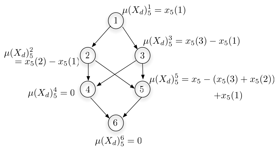
The prediction of at subsystem is and the prediction of at subsystem is . The differential improvement in the prediction of at subsystem regarding the state is . At subsystems the formula for the differential improvement is similar. The differential improvement in at subsystem is zero (since is offstream with respect to ). The differential improvement for at subsystem is zero (since is downstream with respect to ). These differential improvements are depicted in Fig. 4. Capturing these differential improvements is precisely the role of the Möbius operator.
We can now understand the role of (8) better. Let be a local state and let denote the row of . The entry of (i.e. ) corresponds to the prediction of at subsystem , so that the row vector summarizes the predictions of the state at the different subsystems.
Recalling (8), we have
Restricting to the row and rewriting we have that
The natural interpretation here is that in our architecture the “atoms” for state prediction are the differential improvements (or increments) . To compute the state prediction at subsystem one simply “integrates” (via ) the increments corresponding to upstream subsystems . This is depicted in Fig. 5.
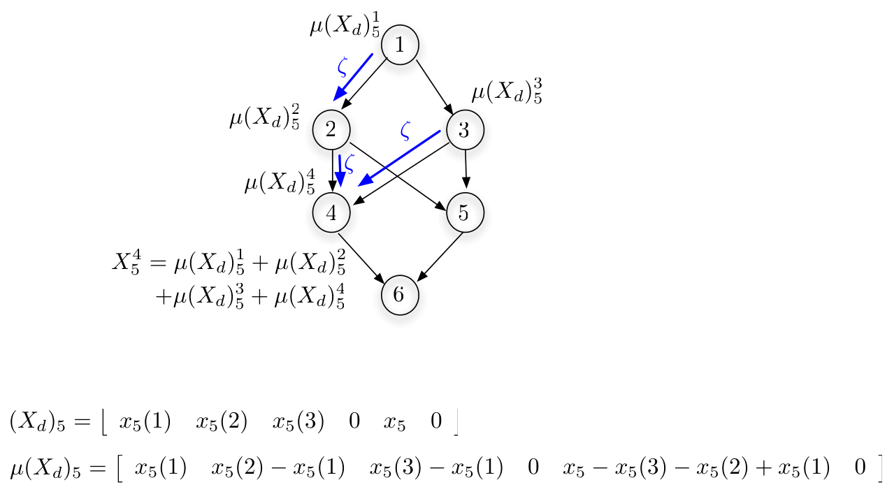
As remarked earlier, our setup ensures that the increment for or if and are not comparable. We briefly explain the intuition behind this. If is upstream of , both subsystem and have access to the full state and hence there is no differential improvement in the state prediction. Furthermore, if and are unrelated, then carries no additional information about and again it is natural to have the differential improvement be zero.
Before we proceed we clarify that the entries of correspond to partial predictions. We clarify the notion of a partial prediction with an example.
Example 8
Consider the system composed of three subsystems with with and (see Fig. 6):

Note that subsystem has no information about the state of subsystem . Moreover, the state or input does not affect the dynamics of (their respective dynamics are uncoupled). Hence the only sensible prediction of at subsystem is (the situation for is identical). However, both the states , and inputs , affect and . Since and are unknown, the state can at best be a partial prediction of (i.e. is the prediction of the component of that is affected by subsystem ). Similarly is only a partial prediction of . Indeed, one can show that is a more accurate prediction of the state , and when suitably designed, their sum converges to the true state .
IV-C Control Law
We now formally propose the following control law:
| (10) |
We make the following remarks about this control law.
- 1.
We note that (10) specifies which amounts to specifying the input for all . It also specifies for which is the prediction of the input at an downstream subsystem .
- 2.
Since is non-zero only on rows and columns in , the controller respects the information constraints. Thus for any choice of gains , the resulting controller respects the information constraints. In this sense (10) may be viewed as a parameterization of controllers.
- 3.
The control law (10) may be alternatively written as . The control law has the following interpretation. If is a minimal element of the poset , then , the vector of partial predictions of the state at . The local control law uses these partial predictions with the gain . If is a non-minimal element it aggregates all the control laws from and adds a correction term based on the differential improvement in the global state-prediction . This correction term is precisely .
Example 9
Consider a poset causal system where the underlying poset is shown in Fig 2(d). The controller architecture described above is of the form (where is a vector containing the predictions of the global input at subsystem ). Noting that , we write out the control law explicitly to obtain:
IV-D State Prediction
Recall that at subsystem the states for are unavailable and must be predicted. Typically, one would predict those states via an observer. However, those states are unobservable; only the state for are observable, and are in fact directly available. In this situation, rather than using an observer one constructs a predictor to predict the unobservable states. These predictions are computed by the controller via prediction dynamics, which we now specify.
Since the dynamics of the true state evolve according to , each subsystem can simulate these dynamics using the local states and inputs. Locally each subsystem implements the dynamics . This can be compactly written as
| (11) |
We remind the reader that , and that (consisting of upstream and offstream components) is determined from via (8). Consequently, the components in are not free variables and one needs to check that (11) constitutes a consistent set of differential equations. Projecting (11) onto orthogonal components using and we obtain
Before checking consistency, we simplify the differential equation for (the “free variables”). The off-diagonal terms in correspond to the predictions of the downstream states, so that this is precisely the equation that governs the prediction or simulation component prescribed in Fig. 1. Simplifying using we get
| (12) |
We think of as the influence of the upstream components (and also the unrelated components) in predicting . The dynamics (12) correspond to the closed-loop dynamics.
IV-E Separation Principle
As a consequence of Lemma 2, we see that and also . Applying to (12) we obtain the following modified closed-loop dynamics in the new variables :
| (13) |
Let us define From (10), and the fact that we will momentarily see that the modified closed-loop dynamics are:
| (14) |
These dynamics describe how the differential improvements in the state evolve. If one picks such that stabilizes , the differential improvements are all stabilized. Thus converges to zero, the state predictions become accurate asymptotically and the closed-loop is also stabilized. We show that (10) achieves this with an appropriate choice of local gains.
Theorem 1
Proof:
Since it follows that
The last equality follows from Lemma 2 and the fact that . As a consequence, for all . Hence the closed-loop dynamics (13) become: ˙ μ(X) ^i(t)=(A+B ^ F (i))μ(X)^i(t).
Recalling that is a local variable so that (viewed as a vector) is non-zero only on it is easy to see that these dynamics are stabilized exactly when are picked such that are stable.
∎
The dynamics of the different subsystems are decoupled, so that the gains may be picked independent of each other. This may be viewed as a separation principle. Henceforth, we will assume that the gains have been picked in this manner. Since the closed loop dynamics of the states are related by an invertible transformation (i.e. ), if the modified closed-loop dynamics (14) are stable, so are the closed-loop dynamics (12).
IV-F Controller Realization
We now describe two explicit controller realizations. The natural controller realization arises from the closed-loop dynamics (12) along with the control law (10) to give:
While the above corresponds to a natural description of the controller, it is possible to specify an alternate realization. This is motivated from the following observation. The control input depends only on . Hence, rather than implementing controller states that track the state predictions , it is natural to implement controller states that compute directly. Hence an equivalent realization of the controller is:
| (15) |
IV-G Structure of the Optimal Controller
Consider again the poset-causal system considered in (16). Recall that the system (1) may be viewed as a map from the inputs to outputs via
where
| (16) |
(We refer the reader to [19] as a reminder of standard LFT notation used above). In this paper we will assume that and . Indeed, this assumption ensures that the plant .
Consider the optimal control problem:
| (17) | ||||||
The solution is the -optimal controller that obeys the poset-causality information constraints described in Section II. The solution to this optimization problem was presented in [10, Theorem 3]. The main idea behind the solution procedure is as follows. Using the fact that are square and invertible (due to the availability of state feedback) it is possible to reparametrize the above problem via . Indeed, this relationship is invertible and the incidence algebra structure ensures that if and only if . Using this the above optimization problem may be rewritten as:
| (18) | ||||||
Using the fact that the norm is column-separable, it is possible to decouple this optimization problem into a set of optimization problems. Each optimization problem involves the solution to a standard Riccati equation. The solution to each yields the columns of , from which the optimal controller may be recovered. An explicit formula for the optimal controller and other details may be found in [9, 14].
In [10], we obtain matrices by solving a system of decoupled Riccati equations via (we use slightly different notation and reversed conventions in that paper, see [10] for details). The optimal solution to (17) is related to the proposed architecture as described below in Theorem 2. Its proof is provided in the appendix.
Theorem 2
Theorem 2 establishes that the controller architecture proposed in this paper is also optimal in the sense of the norm.
V A Block-Diagram Interpretation
We now interpret the separation principle described in Theorem 1 from a block-diagram perspective. We introduce some additional notation to be used in this section. If is a matrix, we denote by to be its standard vectorization via column concatenation. Given matrices and , denotes their Kronecker product, and we recall the standard identity:
Recall the definition of in Definition 6 as being the projection of a matrix onto the incidence algebra. We will abuse notation and also define to be the linear operator that acts on the vectorization and zeroes components whose indices do not belong to the incidence algebra (the usage will be clear from the context).
The elementary blocks that appear in our block-diagram representation are the following:
- •
The plant , which maps the inputs to the states ,
- •
The transfer functions which play the role of predicting the local state variables from the states and inputs for via (12). We call all these transfer functions collectively the “simulator”, because their role may be interpreted as that of simulating upstream states,
- •
The map which takes as input and computes ,
- •
The local gains ,
- •
The map which takes as input and computes .
In the closed-loop system all these transfer functions are interconnected as shown in Fig. 1.
We define the opertators and as follows:
| (19) |
Since , note that (this clarifies the role of inFig. 1). Similarly, . As one might expect, and are invertible restricted to .
Lemma 3
For and as defined in (19)
Proof:
This follows simply by vectorizing the first and second parts of Lemma 2. ∎
Figure 1 explains the closed-loop at block diagram level. The role of the simulator is to form predictions of downstream states from the available states and inputs. These predictions are then processed by , to produce . These are then composed with the local gains to produce . Finally, acts on to produce . Internally within the simulator one can map the downstream components to the local input (using (9)) via
It may be easily verified using (9) that . The overall composition of the plant and the simulator can be combined to give a transfer function which we denote by as shown in Fig 7. It has an explicit formula given by:
| (20) |
Thus is the overall tranfer function that maps (the true and predicted downstream inputs) to (the local states). We illustrate this with an example.
Example 10
As indicated in Fig. 1, the collective map from to (which collects the plant , , and the simulation block into a single transfer function) is simply given by . Thus the block-diagram in Fig. 1 can be simplified to Fig. 7.

The matrix satisfies the following:
Theorem 3
The matrix is block diagonal.
Proof:
Using (20), we have
The last expression is clearly block-diagonal. ∎In terms of this block-diagram approach, the role of and become very transparent: it is simply to diagonalize the map . Once this diagonalization occurs, the controller simply applies a set of diagonal gains to stabilize the closed-loop. This also illustrates the separation principle at the block-diagram level. As mentioned in the preceding discussion, the architecture illustrated in block-diagram Fig 7 is also optimal, in that appropriate choice of the gains yield optimal controllers.
VI Connections to the Youla parameterization
The Youla parameterization (and the related work on purified output feedback [2, 5]) is intimately related to Möbius inversion. We examine their relationship in this section. We begin with a brief review of the Youla parameterization. We will examine the relationship in a discrete-time setting as this will make the presentation much simpler. Consider the system:
| (21) |
For simplicity, we will assume that is stable (this can be easily achieved by choosing a static which is diagonal by picking such that is stable, without affecting the set of achievable closed-loop maps). The Youla parametrization [19, pp. 221-231] exploits the observation that while the set of achievable closed-loop maps is linear-fractional with respect to the controller variable, it is affine in terms of the parameter .
In the case of state-feedback with a stable plant, the Youla parameterization reduces to a particularly simple form, which we now describe. At time , using the information of the state , the controller implements a simulation of the plant to compute a prediction of the state at time via:
| (22) |
Note that the simulation does not have access to the disturbances and hence simply sets it to zero. It then uses the output of the plant (state-feedback) and then computes the difference . It then processes using an arbitrary causal filter and sets the input . This can be summarized using a block diagram as shown in Fig. 8(a).

We point out that the policy is a disturbance feed-forward policy. It has been observed in various papers in the literature that while state-feedback policies may yield a complicated dependence between the closed-loop map and the controller variable, an equivalent reparametrization using disturbance feed-forward policies yields an affine dependence. For example, this observation was made in the context of robust optimization for linear systems in the framework of “purified output-feedback” [2] and also in [4, Chapter 6].
The key step in reformulating a feedback problem into a disturbance feed-forward problem is the explicit reconstruction of the disturbance using the output of the plant and the simulator. This computation may be naturally viewed as a Möbius inversion operation. To the dynamic evolution of the discrete-time system (21) one can naturally associate the poset , i.e. the time-axis indexed by the natural numbers (equipped with the standard ordering). This poset is simply the linear poset indexed by the integers (see Fig. 8(b)), and the system-theoretic notion of causality is simply the specialization of our notion of poset-causality specialized to this poset.
Consider the variable (i.e. the state of the system (21)) as a function on this poset. For elements such that , is available and for elements such that , it is unavailable. Indeed at the element a prediction of may be computed via (this is precisely the role of the simulator described above). Using the Möbius inversion formula for the linear poset we have Hence the disturbance computation may be viewed simply as a Möbius inversion on .
It is possible to extend this interpretation to poset-causal systems with multiple subsystems. In this case, the system of interest is of the form (21), where . The poset associated to the dynamic evolution of this system is then the product poset . An example of product of this is shown in Fig.
9(a).

As explained in earlier sections, subsystems maintain local states which are summarized by the local variable . Using information available at time , the prediction of may be computed as:
| (23) |
However, due to the disturbance, the value of is given by
| (24) |
where . The local state variable may be viewed as a function on the poset , and hence one may define its Möbius inverse with respect to this poset. As a consequence of the product structure of the underlying poset, we have the following important lemma.
Lemma 4
Suppose satisfies (24). Let denote the Möbius operator of the poset . Then
Proof:
We will use to denote the Möbius inversion of the local variable with respect to the poset as defined in Definition 8. It is well-known [7, Proposition 5] that the Möbius operator factorizes for product posets as:
∎Thus the role of the Möbius operator is to compute the local disturbance . Once these disturbances are computed, one may process it using a filter that is causal with respect to to obtain the input . This is depicted in Fig. 9(b).
VII Conclusions
In this paper we considered the problem of designing decentralized poset-causal controllers for poset-causal systems. We studied the architectural aspects of controller design, addressing issues such as the role of the controller states, and how the structure of the poset should affect the architecture. We proposed a novel architecture in which the role of the controller states was to locally predict the unknown “downstream” states. Within this architecture the controller itself performs certain natural local operations on the known and predicted states. These natural operations are the well-known zeta and Möbius operations on posets.
Having proposed an architecture, we proved two of its important structural properties. The first was a separation principle that enabled a decoupled choice of gains for each of the local subsystems. The second was establishing the optimality properties of this architecture with respect to the -optimal decentralized control problem. The proposed Möbius-based architecture is quite natural, has very appealing interpretations, and can be easily extended to more complicated. These extensions will be the subject of future work.
References
- [1] M. Aigner. Combinatorial theory. Springer-Verlag, 1979.
- [2] Aharon Ben-Tal, Stephen Boyd, and Arkadi Nemirovski. Extending scope of robust optimization: Comprehensive robust counterparts of uncertain problems. Math. Program., 107:63–89, June 2006.
- [3] B. A. Davey and H. A. Priestley. Introduction to Lattices and Order. Cambridge University Press, Cambridge, 1990.
- [4] A. Gattami. Optimal Decisions with Limited Information. PhD thesis, Lund University, 2007.
- [5] Paul J. Goulart, Eric C. Kerrigan, and Jan M. Maciejowski. Optimization over state feedback policies for robust control with constraints. automatica, 2006.
- [6] Y.-C. Ho and K.-C. Chu. Team decision theory and information structures in optimal control problems-part I. IEEE Transactions on Automatic Control, 17(1):15–22, 1972.
- [7] G.-C. Rota. On the foundations of combinatorial theory I. Theory of Möbius functions. Probability theory and related fields, 2(4):340–368, 1964.
- [8] M. Rotkowitz and S. Lall. A characterization of convex problems in decentralized control. IEEE Transactions on Automatic Control, 51(2):274–286, 2006.
- [9] P. Shah. A Partial Order Approach to Decentralized Control. PhD thesis, Massachusetts Institute of Technology, (available at http://www.mit.edu/˜pari), 2011.
- [10] P. Shah and P. A. Parrilo. -optimal decentralized control over posets: A state-space solution for state-feedback. Submitted IEEE Transactions on Automatic Control.
- [11] P. Shah and P. A. Parrilo. A partial order approach to decentralized control. In Proceedings of the 47th IEEE Conference on Decision and Control, 2008.
- [12] P. Shah and P. A. Parrilo. A partial order approach to decentralized control of spatially invariant systems. In Forty-Sixth Annual Allerton Conference on Communication, Control, and Computing, 2008.
- [13] P. Shah and P. A. Parrilo. A poset framework to model decentralized control problems. In Proceedings of the 48th IEEE Conference on Decision and Control, 2009.
- [14] P. Shah and P. A. Parrilo. -optimal decentralized control over posets: A state-space solution for state-feedback. In Proceedings of the 49th IEEE Conference on Decision and Control, 2010.
- [15] J. Swigart. Optimal Controller Synthesis for Decentralized Systems. PhD thesis, Stanford University, 2010.
- [16] J. Swigart and S. Lall. Optimal synthesis and explicit state-space solution for a decentralized two-player linear-quadratic regulator. In Proceedings of the 49th IEEE Conference on Decision and Control, 2010.
- [17] H.S. Witsenhausen. A counterexample in stochastic optimum control. SIAM J. Control, 6(1):131–147, 1968.
- [18] H.S. Witsenhausen. Separation of estimation and control for discrete time systems. Proceedings of the IEEE, 59(11):1557 – 1566, 1971.
- [19] K. Zhou and J. C. Doyle. Essentials of Robust Control. Prentice Hall, 1998.
The required optimal solution was derived in [10][Theorem 3] and we first develop some notation and concepts that have been used therein. Let us define (so that the vector has only those components of such that ), and . Note also that from (7). Let us define . The closed-loop dynamics (14) at subsystem reduce to:
| (25) |
Note that from (10) (keeping in mind that if , and that ), the control law assumes the form:
(Recall that is the row of the matrix ). Thus the subsystems need to compute , (the differential improvements in the state predictions at subsystem ) to implement the control law. This is an important feature of the control law: the controller states correspond to the differential improvements rather than the state itself.
It may be verified from (25) and (10) that the explicit controller for subsystem assumes the following form:
| (26) |
Furthermore, note that at subsystem , for . Hence, only the states for need to be computed. Let .
Proof:
As mentioned, the optimal controller is given by [10, Theorem 3]. We will show that when we pick in (15), we recover this controller. In [10], the matrices , , , , , and were defined. It is straightforward to verify that:
Letting be the vectorization of for via , we may rewrite the dynamics in (26) as
| (27) |
Further, note that the vectorization of the control law equation in (26) yields u= [ ∑_k ⪯j K^(j)(↑k, ↑k) [ x_k-∑_l ≺kq_k(l) q(k) ] ]_j ∈P=C_QΠ_2 q+C_Q Π_1(x-C_Φq). Combining the above with (27), we obtain that which is precisely the same expression as the controller described in [10][Theorem 3]. Since this corresponds to the optimal controller, we have the required result. ∎