On the Calogero-Moser solution by root-type Lax pair
Abstract.
The ‘root type Lax pair’ for the rational Calogero-Moser system for any simply-laced root system yields not a solution for the path , but for the values of the inner products , where ranges over all roots of the root system. It does not, however, tell us which value of the inner product corresponds to which root. In the present paper, we show that the solution is indeed uniquely determined by these values (up to root system automorphisms) at almost all times. We show by counterexample that it is possible for two different values of to yield the same set of values for the inner products .
The indeterminacy introduced by the root system automorphisms introduces the interesting question when the path crosses from one fundamental domain into another. We present an algebraic approach for constructing an indicator function containing this information.
1. Introduction
The rational Calogero-Moser system is a system of a finite number of particles on a line, whose pairwise interaction potential at distance is given by . Given certain initial values for positions and momenta , one is interested in finding the coordinates at later times. There is a remarkable way of solving this: it turns out that the coordinates at time are given by the eigenvalues of the matrix
| (1.1) |
where and are constructed from the initial values by
The particles’ paths cannot cross because their interaction potential is infinite when they meet; so at a given time, the unordered set of eigenvalues can be ordered from smallest to greatest to obtain the positions of each particle.
It was observed by Olshanetsky and Perelomov [3] that this method of solution depends crucially on the property that the set of linear maps forms a root system (namely the root system in the case of particles), and that similar methods of solution work for systems whose interaction potential is given by
for other root systems . In [1] and [4], Bordner, Corrigan, Sasaki and Takasaki introduce a a Lax pair that works for all irreducible simply-laced root systems. Their matrices are much bigger, having a row and column for each root in the root system, and are given by
Again defining , the set of eigenvalues of turns out to be equal to the multi-set11 1 By a multi-set, we mean a set together with a map , where we interpret the value of as a multiplicity. When it is clear from the context, we may drop the “multi” prefix. of real numbers
| (1.4) |
where is the path of the position coordinates, and is the inner product in the ambient Euclidean space of . Therefore, once these eigenvalues are known (step 1), and once we know which eigenvalue corresponds to which root (step 2), all that is left is to solve a system of linear equations for (step 3). It is the second of these steps that presently interests us.
First of all, it is clear that the set can only determine up to isometries of that leave invariant; that is, up to root system automorphisms. Therefore, we immediately see that the correspondence is not uniquely defined. Our first task is to show that this is the only indeterminacy. It turns out that this is true only generically; we will show, by a counterexample in the case, that there can be points in that are in distinct automorphism orbits, but that nevertheless have
Our next objective is the following. Since we can solve for only up to the group action, one could say that the natural domain for is instead of . However, for a physical system of particles, this is quite unsatisfactory, as we in general do distinguish initial values even when they are in the same -orbit. (For instance, in the case, we do want to distinguish a solution from its mirror image.) Therefore, we should divide into fundamental domains, and we should find out, for a given initial value, at what time the path will cross the boundary of the fundamental domains. This, together with the initial value, allows us to resolve the ambiguity and reconstruct the path in its entirety.
This task becomes more interesting when we require the following. Note that finding the eigenvalues of a given matrix involves finding the zeroes of a polynomial, which cannot, in general, be done in closed form. We therefore require that we formulate our answer in terms of the coefficients of the characteristic polynomial for (for which we do have explicit formulae) and not in terms of the eigenvalues of
2. Example: The case

Let us discuss the problem that we are trying to solve in the case where is the root system associated to . This root system is most naturally descibed in the Euclidean subspace satisfying . The root system is given by the set of vectors , , in , and the interaction term in the Hamiltonian is
The Weyl group is and it acts by permuting the coordinates (which clearly leaves the Hamiltonian invariant), and the nontrivial Dynkin diagram automorphism acts by sending . Together, they generate the root system automorphisms . Note that a Weyl chamber is a fundamental domain for the action of the Weyl group, whereas either half of the Weyl chamber is a fundamental domain for the action of the entire .
Figure 2.1 depicts a path in and the other paths in its orbit. The orbit consists of six paths because of the group action alone, and this number is doubled by the Dynkin diagram automorphism. It is clear that at a given time , all these values for yield the same set for . In the case, it is easy to see that conversely, two values giving the same set are in the same -orbit: after choosing a Weyl chamber, the maximal value in must be associated to the maximal root. After this, there are only two positive values left, which can be assigned in exactly two ways to the two positive roots. In larger root systems, this converse is not so obvious – in fact, it is false in general. We will discuss this issue in section 3.
The shaded area is a Weyl chamber, given by . It is easy to distinguish paths in different Weyl chambers, because the Hamiltonian is infinite along the borders; if the initial value of a path is in a particular Weyl chamber, the path will stay there for all time. However, this does not allow us to distinguish the two paths in the same Weyl chamber, related by . We will tackle this problem as follows. First, we identify a hyperplane that separates one fundamental domain from the other. In the case, this hyperplane is just the line of fixed points, but in general, the fixed points are only contained in this hyperplane22 2 Here, we restrict to root systems having exactly 2 Dynkin diagram automorphisms. The case of only a single automorphism is trivial, so we only exclude the case.. Next, we try to identify the times at which the paths cross this hyperplane. (In general, the paths do not need to intersect each other as they do in the case.) The result obtained in section 5 will be a real polynomial with zeroes exactly where this happens. Assuming these are simple zeroes, this means that this polynomial takes positive values at times where we should take one fundamental domain, and negative values when we should take the other.
3. Indeterminacy of the solution
Let be an irreducible, simply-laced root system in a Euclidean space . Simply-laced means that all roots have ; it can be shown that this implies the following relations that we will use:
- •
if , then ;
- •
if , then ;
- •
otherwise (i.e. if ), we have .
Suppose that we are given a multi-set of real numbers, and we know that it is equal to some of the form (1.4) (we will drop the time-dependence in our notation in this section). Another way to say this is that there is a bijection such that
| (3.1) |
Here, the word ‘bijection’ should be interpreted as: is a map from to the underlying set of , such that the size of the preimage of each point is equal to its multiplicity in . Given such a bijection, we can solve for . In fact, is already determined by its inner products with the simple roots , since these are linear equations for unknowns.
It is clear that if is a root system automorphism, then will be another bijection that satisfies (3.1). The converse needs proof:
Proposition 3.1.
The following statement is true for generic : If and are two bijections satisfying (3.1), then there is an automorphism such that .
Note that in the case where has multiple values, the condition does not even fix as a bijection, so it is not an entirely trivial matter to find a suitable . The proof will need the following definition and lemma.
Definition 3.2.
Let be any map. We call additive if it satisfies these conditions:
for any value of such that is a root, and
for any .
It is important to realize that is not a group under addition. In particular, this means that the second condition does not follow from the first.
Lemma 3.3.
The following statement is true for generic . Suppose is a bijection such that . Then is additive.
Proof.
First of all, note that from (3.1), it follows in particular that the are additive, in the sense that and . However, this does not imply that is additive: it is possible that
even if is not a root. In this case, cannot equal .
We write for the free abelian group with a set of generators indexed by . There is a canonical map to the root lattice, whose kernel contains exactly the additivity relations. The map induces a map . It is easy to see that is additive if and only if maps to itself, in other words, if and only if
Now let us consider the . We see that each extends linearly to a map (we use their additivity here). The statement that implies that we have the following commutative diagram:
The dotted arrow is a map that exists if and only if is additive.
We see from the diagram that
This means that
so it is sufficient if we can prove that is trivial.
Note that is generated by linear combinations of at most 3 generators. This means that it is actually sufficient to show that does not contain elements that small. In fact, preserves norms and only makes them smaller, so it is sufficient if does not contain elements of length smaller than .
Now, is a hyperplane of codimension 1 in the ambient space of the root lattice . For generic values of ’s coefficients , this hyperplane has trivial intersection with
This means that
for generic . This implies that is additive. ∎
Proof of proposition 3.1.
Choose any that satisfies , and choose a a base for the root system. There is a unique linear map that extends on . Because is additive, we see that actually extends on all of . We will now show that is an isometry. We can check this on because these roots span . Because extends a permutation of the roots, it is clear that if and only if . But in light of the relations above, this means that
so is an isometry and is an automorphism of . ∎
Now remember that the Hamiltonian has a pole along for every root , that is, along the boundaries of the Weyl chambers. This means that if the initial value for is in a certain Weyl chamber, then it will stay there for all . This means that we can fix a set of positive roots corresponding to the Weyl chamber, and use an element of the Weyl group to make sure our bijection sends positive roots to positive values of . This will make sure that the corresponding solution for is in the right Weyl chamber. This proves the following
Proposition 3.4.
For generic , there are exactly possibilities for the solutions for . They are related by the action of the Dynkin diagram automorphisms on .
4. A non-generic counter example
The question remains whether the proof of lemma 3.3 can be made to work for all, instead of just generic, . The answer to this question is negative, at least for the case . In this case, consider the vectors
which are not mirror-images and therefore not related by a Dynkin diagram automorphism. Then we can check that
For reference, both are equal to the multi-set
| (4.1) |
This counter-example was produced by computer-search33 3 The search was conducted using the open-source software Sage [5]. Source code for the search program is available from the author’s website.. A non-exhaustive search for counterexamples in other small root systems ,, and did not yield any other examples.
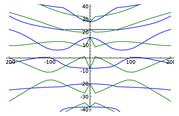
A natural question is how the path evolves when we take these two points as initial values. The two different are diagonal matrices that have the numbers (4.1) as eigenvalues, but on different rows. There is no similar relation between the two different , because the map on induced by the correspondence does not respect additivity relations. Therefore, there is no reason to suspect that the two solutions remain related in any way. This is illustrated in figure 4.1.
5. Fundamental domain crossings
Let us now exclude the cases (which only have the trivial diagram automorphism) and the case (which has 6 automorphisms) so that we have exactly 2 solutions for at every time . In other words, we have a path in the quotient space
We would like to separate the two “lifted” paths in the Weyl chamber. One way of doing this is to split the Weyl chamber into two fundamental domains, and finding out at what time passes the boundary from one fundamental domain to another. The Dynkin diagram automorphism corresponds to a linear isometry of order 2, so we can choose the fundamental domains as being the two sides of any codimension 1 hyperplane containing its fixed points44 4 To see this: if two points are on the same side of the hyperplane and are mapped to each other, then their sum is also on the same side of the hyperplane, but it is a fixed point.. In fact, we can always take the hyperplane to be the equidistant hyperplane between two simple roots forming an orbit. For example, in the case, we can choose the boundary of the fundamental domains to be the dotted line in figure 2.1. We then want to find the times at which the paths cross the boundary. We have seen in the case that they must cross each other because the boundary is actually fixed by the automorphism. In general, however, the boundary need only be mapped into itself, so the paths can cross the boundary at distinct points.
We would like to express the fact that is on the boundary by looking at the values of . Then because the boundary is an equidistant hyperplane, we see that there must be double values. The converse is false, however: there are several more equidistant hyperplanes, but not all of them are between roots in an orbit, and from those that are, we have only chosen one as the boundary of the fundamental domain. Also remember that we want to find a condition on the coefficients of the characteristic polynomial of ; that is, on the symmetric functions of the , and not on the themselves.
5.1. An algebraic condition for the crossing
There is a standard way of expressing certain conditions on the zeroes of a polynomial as conditions on coefficients. Let us illustrate this method by recalling the definition of the discriminant of a polynomial. Consider a polynomial
We can express the condition that this polynomial has a double zero (that is, there is with ) by requiring the vanishing of the following expression
which is symmetric in the and can therefore also be expressed in the . This expression is just a power of the determinant.
Let us apply this to the the condition that is at the boundary of a fundamental domain. This is a condition on the zeroes of the form:
There is a way of assigning the to roots such that (1) the satisfy the additivity properties of the roots and (2) they have the same value on two specified roots.
For example, in the case, we want the simultaneous vanishing of these expressions:
| (5.1) | (one root is the sum of two other roots) | ||||
| (those two other roots have the same value) | |||||
| (the roots have mirror images) | |||||
| (idem) | |||||
| (idem) |
The second of these corresponds to (2), and the others correspond to (1). Of course, vanishing of a simultaneous permutation is also allowed, since that corresponds to a different way of assigning roots to the . The simultaneous vanishing of any simultaneous permutation can be encoded in the vanishing of the following expression:
identically in the helper variables . Taking the product over all permutations makes that the condition is symmetric in the , allowing us the express it in the . Note that the identical vanishing will give one condition for every monomial in .
Now in general, suppose the additivity relations (such as (5.1) in the case) take the form for in some index set , and suppose that the boundary hyperplane is equidistant to . Then we are interested in the vanishing of the following expression:
| (5.2) |
identically in the helper variables . Again, this condition can be expressed in the , and we obtain one condition for every monomial in the . In our case, the coefficients are the coefficients of the characteristic polynomial of . That means that we have explicit formulae . These are polynomials in with coefficients in , where and are the initial values.
Since is a unique factorization domain, there is a well-defined greatest common divisor of all the . This greatest common divisor vanishes exactly when is on the boundary of the fundamental domain at time . This is a real polynomial with zeroes exactly at boundary crossings. Assuming the zeroes are simple, we can interpret it as an indicator function that is positive at times where the path is in one fundamental domain, and negative when it is in the other.
5.2. Feasibility of the computation
The computation just described is unfeasible, even for the smallest of root systems. In the case , we have roots, so the expression (5.2) is a homogeneous polynomial of degree in the 6 -variables, which means it has summands, a 13 digit number.
A polynomial whose computation is a lot closer to being within reach is the discriminant of the characteristic polynomial of . It is zero exactly at times when has double values. In particular, it is zero when crosses a boundary. We find that is a factor in . Furthermore, because we have just shown that is a polynomial in , we can obtain by factoring over . When we fix rational values for the initial values and , this is a factorization over and so it is a finite computation.
As an example of this procedure, let and let the initial values be given by and . Because these are rational values, is just equal to . The charateristic polynomial of with these initial conditions can be computed to be equal to
The discriminant of this polynomial is equal to
for some large constant . A numerical approximation of the solution shows that we expect that the fundamental domain border is crossed three times. This allows us to identify the factor of degree 3 as the indicator function that is positive when the solution is in one fundamental domain, and negative when it is in the other. This is a less rigorous way because it involves comparison of an exact result with a numerical approximation, but it is at least feasible.
6. Conclusion
We have shown that the solution to the Calogero-Moser system by root-type Lax pair is complete up to root system automorphism, in the sense that the data it yields determines the solution at almost all times (and therefore by continuity at all times); however we have shown by example that ambiguity can occur at isolated points.
Next, in the cases where there are exactly two different Dynkin diagram automorphisms (so in all cases different from ), we have given a way of distinguishing the two paths in the Weyl chamber by means of an indicator function, whose construction is entirely algebraic. However, its computation is infeasible even for tiny examples, but we have also indicated a less rigorous way of obtaining it in a much less computationally expensive way.
It is known that in cases different from , an alternative Lax pair is available (called the minimal Lax pair in [1]) that yields not values for , but for where runs over the fundamental weights. It would be interesting to see if similar steps are necessary to ensure that the resulting data completely fix the solution.
7. Acknowledgements
This research was helped by computer exploration using the open-source mathematical software Sage [5] and its algebraic combinatorics features developed by the Sage-Combinat [2] community. In particular, the work by Mike Hansen, Justin Walker and Nicolas M. Thiery on root systems was very helpful.
Source code for an implementation of the above algorithm in Sage is available from the author’s website55 5 This website can be found at www.staff.science.uu.nl/~kluck103/.
This research was supported by the Utrecht University program ‘Foundations of Science’.
References
- [1] A. J. Bordner, E. Corrigan, and R. Sasaki, Calogero-Moser Models I. A New Formulation, Progress of Theoretical Physics 100 (1998), no. 6, 1107–1129.
- [2] The Sage-Combinat community, Sage-Combinat (Version 4.6.2): enhancing Sage as a toolbox for computer exploration in algebraic combinatorics, 2011, http://combinat.sagemath.org.
- [3] M. A. Olshanetsky and A. M. Perelomov, Classical integrable finite-dimensional systems related to Lie algebras, Physics Reports 71 (1981), no. 5, 313–400.
- [4] R. Sasaki and K. Takasaki, Explicit solutions of the classical Calogero and Sutherland systems for any root system, Journal of mathematical physics 47 (2006), 012701.
- [5] W. A. Stein et al., Sage Mathematics Software (Version 4.6.2), 2011, The Sage Development Team, http://www.sagemath.org.