Wavepacket approach to particle diffraction by thin
targets:
quantum trajectories and arrival times
Abstract
We develop a wavepacket approach to the diffraction of charged particles by a thin material target and we use the de Broglie-Bohm quantum trajectories to study various phenomena in this context. We construct a particle wave function model given as the sum of two terms , each having a wavepacket form with longitudinal and transverse quantum coherence lengths both finite. We find the form of the separator, i.e.the limit between the domains of prevalence of the ingoing and outgoing quantum flow. The structure of the quantum-mechanical currents in the neighborhood of the separator implies the formation of an array of quantum vortices (nodal point - X point complexes). The X point gives rise to stable and unstable manifolds, whose directions determine the scattering of the de Broglie - Bohm trajectories. We show how the deformation of the separatior near Bragg angles explains the emergence of a diffraction pattern by the de Broglie - Bohm trajectories. We calculate the arrival time distributions for particles scattered at different angles. A main prediction is that the arrival time distributions have a dispersion proportional to the largest of the longitudinal and transverse coherence lengths, where is the mean velocity of incident particles. We also calculate time-of-flight differences for particles scattered in different angles. The predictions of the de Broglie - Bohm theory for turn to be different from estimates of the same quantity using other theories on time observables like the sum-over-histories or the Kijowski approach. We propose an experimental setup aiming to test such predictions. Finally, we explore the semiclassical limit of short wavelength and short quantum coherence lengths, and demonstrate how, in this case, results with the de Broglie - Bohm trajectories are similar to the classical results of Rutherford scattering.
Keywords:
Particle diffraction; de Broglie - Bohm trajectories1 Introduction
The de Broglie - Bohm quantum trajectories [1] [2][3][4] have been considered as an interpretational tool in a number of recent applications (see [5][6][7] for reviews), since they can offer new insight into a variety of complex quantum phenomena. According to the de Broglie-Bohm theory, to any wavefunction describing a particle system, we can associate a set of ‘quantum trajectories’. One trajectory is defined by the initial conditions and by the ‘pilot wave’ equations of motion
| (1) |
where are the particle masses and is Planck’s constant. The equations of motion (1) imply the continuity equation for the probability density . In particular, in a one-particle system we can choose many different initial conditions corresponding to an initial density . Then, the pilot-wave equations guarantee the preservation of Born’s rule at all subsequent times . Furthermore, the de Broglie - Bohm trajectories are equivalent to the stream lines of the quantum probability current . Thus, the Bohmian approach yields practically equivalent results to Madelung’s quantum hydrodynamics [8].
The de Broglie - Bohm theory has been discussed extensively from the point of view of its relevance as a consistent interpretation of quantum mechanics (e.g. [4], [9]; see [10] for an extended list of references). However, the employment of the de Broglie - Bohm trajectories has been proven useful also in many practical aspects of the study of quantum systems. Some modern applications are:
i) Visualization of quantum processes: examples are barrier penetration or the quantum tunneling effect [11] [12][13][14], the (particle) two-slit experiment [15], ballistic transport through ‘quantum wires’ [16][17], molecular dynamics [18], dynamics in nonlinear systems with classical focal points or caustics [19], and rotational or atom-surface scattering [20] [21][22].
ii) Lagrangian solvers of Schrödinger equation via swarms of evolving Bohmian trajectories (see [5] for a comprehensive review, as well as [23] [21][22][24]). The interest in this method lies in that, instead of solving Schrödinger’s equation first, one uses a step-by-step procedure to calculate the trajectories via Newton’s second order equations of motion in a potential
| (2) |
where is the ‘quantum potential’, caused by the wavefunction :
| (3) |
Using the information of the initial value of the wavefunction as well as the evolution of the quantum trajectories, the wavefunction can then be determined at any subsequent time step.
iii) Dynamical origin of the quantum relaxation [25] [26][27][28][29]. The de Broglie - Bohm theory offers a justification of Born’s rule , since it predicts that, under some conditions, the quantum trajectories lead to an asymptotic (in time) approach towards this rule even if it was initially allowed that . It should be noted that not all choices of are guaranteed to lead to quantum relaxation, and counter-examples can be found, for reasons explained in [26]. The arguments used in that paper to explain the suppression of the quantum relaxation effect in the two-slit experiment apply also to many other cases (see e.g. [30]). In particular, a necessary condition for quantum relaxation to take place is that the trajectories should exhibit chaotic behavior (see [25] [26]); however, even this condition is not sufficient (see [31]). The problem of chaos in the de Broglie - Bohm theory has been studied extensively (indicative references are [32][33][34][35] [36][37][38][39] [40][41][42][43] [44][45][46][47]). We have worked on this problem in [26][48] [49][50][51]. Our main result was that chaos is due to the presence of moving quantum vortices forming ‘nodal point - X-point complexes’ ([48][49][50]; see also [45][46]). Quantitative studies of chaos and of the effects of vortices are presented in [38][47][50]. In particular, in [50] we made a theoretical analysis of the dependence of Lyapunov exponents of the quantum trajectories on the size and speed of the quantum vortices, thus explaining numerical results found in [48] and [49]. Furthermore, in [26] we gave examples of systems which do or do not exhibit quantum relaxation, depending on whether or not their underlying trajectories are chaotic. It should be emphasized that, besides chaos, the quantum vortices play a key role in a variety of quantum dynamical phenomena (e.g. [52][11] [53][21][22]).
iv) Arrival times and times of flight. In the traditional formulation of quantum mechanics time is only a parameter in Schrödinger’s equation, since by a theorem of Pauli [54] no definition of a self-adjoint time-operator consistent with all axioms of quantum mechanics can be given in a system with energy spectrum bounded from below. Time, however, is an experimental observable. Various approaches in the literature, reviewed in [55][56], have addressed the question of a consistent definition of quantum probability distributions for time observables. Besides the Bohmian approach, two other approaches are: a) the ‘sum-over-histories’ approach [57][58] based on Feynman paths, and b) the approach of Kijowski [59], based on the definition of quantum states acted upon by the so-called ’Bohm-Aharonov operator’ (see [55]). On the other hand, the de Broglie - Bohm approach gives a straightforward answer to this problem, since the time needed to connect any two points along a quantum trajectory is a well defined quantity (see [60] [61]).
Regarding this latter point, a key remark that will concern us in the sequel is that a consistent definition of the arrival times, that would allow in principle for a comparison of the various approaches in specific quantum systems, is only possible provided that the initial wavefunction is localized in space, i.e. it is described by a wavepacket model.
Being motivated by the latter remark, in the present paper we present a study of the de Broglie - Bohm trajectories in a wavepacket model referring to a quantum phenomenon that has played a fundamental role in the development of quantum mechanics, namely the diffraction of charged particles (e.g. electrons or ions) by a thin material target.
A theoretical study on the quantum scattering problem in the framework of the de Broglie - Bohm approach has been presented in the series of works [62][63][64] [65][66]. These studies refer to the establishment of the rules of scattering probabilities using the ‘flux across surfaces’ theorem adapted to the concept of quantum trajectories. However, they do not deal with the form of the quantum trajectories or the emergence of diffraction patterns under specific scattering potentials. A numerical simulation of Rutherford scattering by a single nucleus has been presented in [67], while in [23] the phenomena of atom-surface scattering as well as neutron diffraction by slits are considered, which share some common features, but also important differences, with our problem.
In the present paper we make a detailed study of the de Broglie - Bohm trajectories in the context of a wavepacket model of charged particle diffraction, by first investigating the form of the quantum currents corresponding to various cases of this model. These cases are diversified one from the other by the different quantitative relations characterizing the so-called quantum coherence lengths in the longitudinal and transverse directions of the charged particle beam. This is necessary in order to be able to compare the results corresponding to possibly different experimental realizations of a charged particle beam, as e.g. in the case of electrons produced either by thermionic or by a cold-field emission processes.
Our present study completes in a substantial way the study initiated in a previous paper of ours [51], in which we implemented the de Broglie - Bohm approach in the case of electron diffraction through a thin crystal. In that study, however, we assumed a planar wave model for the propagation of the electron wavefunction in the longitudinal direction. In contrast, in the present paper we assume instead a finite longitudinal quantum coherence length. This assumption leads to a number of crucial new elements with respect to [51]. In fact, in order to achieve our goal we derive a wavefunction model by a refined implementation of basic scattering theory, so as to account for a fully-localized in space description of scattering. The derivation of this model presents its own interest, and it is exposed in detail in section 2.

The structure of the paper is as follows: after the derivation of the basic wavefunction model in section 2, we pass to a study of the quantum trajectories in section 3. Here the emphasis is on the influence upon the trajectories of quantum vortices, whose appearance and role in this problem are explicitly discussed. In fact, we show that the quantum vortices appear in the transition zone from a domain of predominance of the ingoing wavefunction to a domain of predominance of the outgoing wavefunction. Inside this zone we can define a locus called separator, which plays a key role in the interpretation of the scattering process via the quantum trajectories. In section 4 we study the arrival times of diffracted particles to detectors placed in various scattering angles. A main outcome of this study is that it is possible to propose a feasible experimental test probing the predictions of the Bohmian theory about the particles’ arrival times. In section 5 we discuss separately the ‘semi-classical’ case of particles with a large mass and and a small de Broglie wavelength, applicable e.g. to particle or ion scattering, since this case exhibits some special features in comparison to the case of electron diffraction. Finally, section 6 summarizes the main conclusions of the present study.
2 Modelling of the wavefunction
We consider a cylindrical beam of particles of mass and charge incident on a thin material target. We set the center of the target as the origin of our coordinate system of reference, and use both cylindrical coordinates and spherical coordinates . The axis is the beam’s main axis, denotes cylindrical radius transversally to , is the azimuth, and (see Figure 1, schematic).
A basic form of diffraction theory for charged particles, reviewed e.g. in [68], assumes that the incident waves are planar. As explained in the introduction, here instead we are interested in a wavepacket approach. Focusing only on elastic scattering phenomena, the latter approach can be obtained by a refinement of the basic theory as follows:
The potential felt by a charged particle approaching the target can be considered as the sum of the individual potential terms generated by every atom in the target:
| (4) |
where denotes the position of j-th atom in the lattice of the target (this position exhibits some statistical fluctuations due to thermal oscillations etc; the effect of these fluctuations is discussed later in this section). As a model for the function , we can adopt a screened Coulomb potential
| (5) |
( = vacuum dielectric constant), where is the
nuclear charge, and is a constant representing a charge
screening range within the atoms, whose value is of the order
of the atomic size.
Particles being scattered by the target can be described by a wavefunction given as a superposition of eigenfunctions
| (6) |
where are Fourier coefficients, and are scattering eigenfunctions, i.e. solutions of the time-independent Schrödinger’s equation
| (7) |
with chosen as in (4) and . The different solutions are labeled by their wavevectors of modulus , where is the energy associated with one eigenstate. Born’s approximation can be used to obtain an approximative formula for . We thus write
| (8) |
where is the solution of Eq.(7) for the free particle problem , while , etc (assuming that small compared to the particles’ energies). The above series are meaningful at all points of space excluding a set of balls of radius a few times around every one of the atoms in the target. Spherical harmonic expansions (see e.g. [69]) provide a more accurate representation of the solution inside such balls, but their use is cumbersome while practically unnecessary in the context of the present study.
A step by step determination of the series terms in (8) can be obtained via the recursive formula
| (9) |
All essential phenomena discussed below are present already in the solutions including just the two first terms . From Eq.(9) for we find:
| (10) |
The integral in (10) can be estimated using standard approximations of scattering theory. We then find
| (11) |
where denotes the angle between the vectors and .
Substituting Eq.(11) into Eq.(6) we have
| (12) | |||||
The problem of defining is now restricted to making an appropriate choice for the coefficients . The latter are determined by the Fourier transform of the initial wavefunction . In the wavepacket approach, the initial wavefunction is localized around the source, i.e. far from the target. Hence we can set , where represents a wavepacket moving in the z-direction towards the target with some velocity . A Gaussian wavepacket of this form corresponds (in momentum space) to the choice
| (13) |
In (13), are the Cartesian components of , is the initial position of the center of the wavepacket along the z-axis, and . The quantities , are the longitudinal and transverse dispersions of the wavepacket in momentum space. These correspond to dispersions in position space given by and . The quantities and are hereafter called the longitudinal and transverse quantum coherence length respectively. Eq.(12) now takes the form
| (14) |
where
| (15) |
with
The function corresponds to the second integral in (12). An explicit expression for this function can only be found by adopting some further approximations. First, we consider fast-moving wavepackets, for which as well as . Then, in the denominator of the second integrand in (12): i) the term can be ignored, and ii) we use the approximation . Second, at all distances we have that the angles are approximately equal one to the other and to the angle (which is equal to the angle between the vectors and . Finally, we set in the exponential argument of (12), where (this is necessary in order to retain all terms whose phase has a substantially non-zero value), while we set in the denominator of the integrands in (12). Using these approximations, we find
| (16) | |||||
where represents the mean velocity of a particle with wavenumber .
At distances closer to the target than the maximum of the two coherence lengths , the prefactor in Eq.(16) is no longer accurate. In order to be able to perform some numerical calculations of de Broglie - Bohm trajectories, after numerically simulating the sums appearing in (12) we found by trial a fitting model that represents reasonably well the modifications of close to the target. This reads:
| (17) |
where and are fitting constants determined by comparison of Eq.(17) to the results of the numerical simulation of (in all simulations below we set , ). It is to be stressed that Eq.(17) correctly recovers the asymptotic form when is large.
The outgoing wavefunction now takes the form
| (18) |
where the quantity is called hereafter the ‘effective Fraunhoffer function’ (in analogy with the ‘far field’ diffraction limit in wave optics, see [70]). This is given by
| (19) | |||||
The physical significance of the function is that it sums the contributions of all the atoms in the target which act as sources of partial outgoing waves, whose superposition forms . Furthermore, the function accounts for the formation of a diffraction pattern, which, for given , , arises by the coherent contributions of all atoms in the target whose phasors are nearly parallel one to the other. As in [51], we consider the simplest example of a cubic lattice structure of the target
where i) is the lattice constant (equal to the length of one side of the primitive cell) ii) is the amplitude of some random oscillations (due to thermal or recoil motions; is taken equal to a small fraction of ) and are random variables with a uniform distribution in the intervals (the random oscillations introduce a so-called Debye-Waller effect, analyzed in [51]; here, for simplicity, we ignore modifications on the wavefunction due to this effect). iii) The number of atoms in the z-direction is , where is the target thickness, and iv) the value of is of order , due to the Gaussian factor in Eq.(19) which can be approximated by for all and , and by for or (for typical magnitudes of the inequality holds for all times of interest in our study, see below). We now distinguish the following cases:
2.1
When the longitudinal coherence length is larger than the transverse coherence length , a simple modeling of the sum in Eq.(19) becomes possible at all distances . Ignoring first the random fluctuations in (2) (i.e. setting ), we have whereby it follows that
| (21) | |||||
For a random choice of , the total number of contributing atoms in the sums of Eq.(21) is of the order . Furthermore, the phasors have an effectively random phase. Thus, the total sum is of order , and we are lead to the simple estimate
called, hereafter, the ‘diffuse term’ of the effective Fraunhofer function. Using this term we have
| (22) |
where is the number density of the atoms in the target.
The model (22) is used in a number of numerical simulations below. It describes a radial pulse propagating outwards with speed , which emerges from the center at the time . It should be stressed, however, that Eq.(22) requires modifications close to particular angles where the phasors in the sums of (21) are added coherently. This will be examined in subsection 3.3. Further modifications are required when and become comparable or smaller than the inter-atomic distance in the target. This case is examined in section 5.
2.2
The modeling of is a more subtle problem if the transverse coherence length is larger than the longitudinal coherence length. Without loss of generality, we can consider a fixed meridian plane defined e.g. by the angle . We set and we make the change of variables , . Considering now a random choice of , and ignoring the quantity , for a given value of the sum over the variables in Eq.(19) can by approximated by a sum over a domain of values of such that belongs to a ball of radius around . The total number of contributing atoms is then of order . If i) we consider the sum over the phasors as a sum of random numbers (yielding a total magnitude ), and ii) we substitute the second exponential in (19) by a delta function around , we find , where
| (23) |
and is the determinant of the Jacobian matrix of the transformation . We find
| (24) |
where , . Eq.(24) yields non-zero values of the integral below a cut-off radius . However, the asymptotic behavior of when is large is found by noticing that and in this limit. We then find
| (25) |
The essential point to retain is that the profile of the radial outgoing pulse in the case is a Gaussian whose dispersion is of order . Thus, the conclusion is that, in both cases or , the outgoing wavefunction has always the form of a packet with dispersion of the same order as the largest of the two quantum coherence lengths, i.e. .
Furthermore, we notice that in the case the dispersion depends also on . A detailed investigation of the Bohmian trajectories in this case is, however, not possible from a numerical point of view, because the asymptotic formulae (24) and (25) are not valid at distances , where the scattering effects take place. Thus in the sequel we limit ourselves to a detailed investigation of the Bohmian trajectories in the case , while a qualitative discussion of the case will be made in section 4, referring to the issue of the particles’ arrival time distribution.
3 Quantum trajectories
We now discuss the main features of the de Broglie - Bohm quantum trajectories focusing on the case .
3.1 Separator and quantum vortices
The form of the trajectories can be found by carefully examining the structure of the quantum currents . The main remark is that, due to Eqs.(15) and (22), the ingoing wavefunction term (which has a Gaussian form both in the and directions) has a falling exponential profile at large distances from the center of the Gaussian, while the outgoing wavefunction has a more complex form falling asymptotically as a power-law due to the factor . Thus, there is an inner domain of the quantum flow where prevails, and an outer domain where prevails. We call separator the boundary delimiting the two domains. Formally, the separator is defined as the (time-evolving) geometric locus where
| (26) |
In the case where the outgoing wavefunction is given by Eq.(22), the condition (26) takes the form:
| (27) |
where we use the approximations and . We note that these approximations hold within a range of parameter values relevant to concrete experimental setups. For example, assuming that incident particles have velocities of order m/s, the time required to travel a distance of order – m (which is the typical size of an experimental setup) is of the order of – s. On the other hand, the typical coherence lengths in experiments e.g. for electrons are of order 1m or larger. Hence, is much smaller than or .

The time evolution of the separator in the plane depends now on the time evolution of the relative amplitude of the ingoing compared to the outgoing wave at any point of the configuration space. We note first that according to Eq.(22), the outgoing wave corresponds to a wavepacket with dispersion which emerges from the center in the time interval , with , , which is the interval during which the support of the ingoing wavepacket (moving from left to right in Figs.1 and 2) essentially overlaps with the spatial domain occupied by the atoms in the target (see [69] for an introductory description of this phenomenon in a simple Rutherford scattering case). As indicated by Eq.(22), after its emergence the outgoing wave moves in all radial directions maintaining essentially its Gaussian profile, while its overall amplitude drops like . As the outgoing wave moves outwards, it first encounters the ingoing wavepacket at times close to . In Fig.2a, this encounter results in a gradual approach of the separator towards the z-axis (the indicated times are , , ). As, however, the ingoing packet moves from left to right in Fig.1, its center crosses the target at the time . Afterwards, the ingoing wave emerges from the right side of the target, and its support lies nearly completely in the semi-plane . At a still longer time (), the center of the outgoing wavepacket has traveled a distance apart, and there is no longer any overlapping between the ingoing and outgoing wavepackets. As observed in Fig.2a, a transition takes place at some time between and , such that, before the transition, the separator is formed by a a pair of open curves on either side of the axis , while after the transition there is only one closed curve intersecting twice the axis both for and . Taking into account the cylindrical symmetry around the z-axis, the form of the separator in space before the transition is a cylindrical-like surface of rotation, while after the transition it becomes a prolate spheroidal-like surface. In fact, this time-changing surface marks a sharp limit between the domains of prevalence of the axial ingoing flow and the radial outgoing flow, as shown in Fig.2b for the time .
If Eq.(27) is supplemented by an equation for the phases of the ingoing and outgoing waves, which, for takes the form
| (28) |
a simultaneous solution of Eqs.(27) and (28) defines the set of all points of the configuration space where the total wavefunction (Eq.(14)) becomes equal to zero. Such points are called ‘nodal points’.
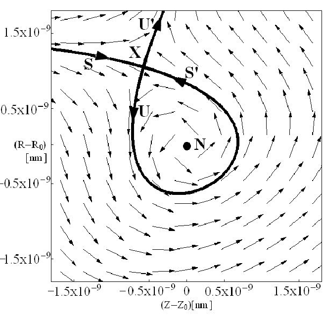
Around the nodal points, the quantum flow forms quantum vortices (Figure 3). The local form of the quantum currents in a vortex domain is very different from the general flow shown in Fig.2. If we ‘freeze’ the time , the instantaneous pattern formed by the vector field of quantum probability current corresponds to a characteristic structure called quantum vortex, or nodal point - X-point complex [48][49][50]. That is, close to a nodal point we find a second critical point of the flow, where one has . This is called an ‘X-point’, since it can be shown that it is always simply unstable, i.e. there are two real eigenvalues of the matrix of the linearized flow around X, which are one positive and one negative. Accordingly, there are two opposite branches of unstable (U,U’) and stable (S,S’) manifolds emanating from X. On the other hand, the nodal point can be an attractor, center, or repellor. This determines the local form of the invariant manifolds U and S. It has been established theoretically [48] that, except for a set of very small measure, most quantum trajectories avoid the nodal point, being instead scattered along the asymptotic directions of the manifolds of the X-point, leading to large distances from the nodal point - X-point complex. Furthermore, while, in general, the motion of the nodal point - X-point complexes introduces chaos ([38][45] [48][50]), in the present problem this effect is negligible because i) the speed of vortices is extremely small (of order ), and ii) the quantum trajectories exhibit only a small number of encounters with nodal point - X-point complexes, as will be shown with numerical examples below. In conclusion, the effect of the nodal point - X-point complexes on the trajectories can be described as a scattering process without recurrences.
For the model parameters used in Fig.3, the size of the quantum vortex, estimated by the distance from the nodal point to the X-point, is of the order of m. The size of vortices in the present model is in fact time dependent. However, in the time interval when there is essential overlapping of the ingoing and outgoing wavefunction terms, is approximately constant and it is given by the same estimate as in the second of the equations (25) of ref.[51], namely
| (29) |
The above estimate is obtained by expanding the wavefunction around a nodal point up to terms of second degree in and , where are the coordinates of the nodal point, and by applying general formulae derived in [50] regarding the dependence of on the coefficients of this local expansion.
3.2 Trajectories

The deflection of an orbit happens at the crossing of the separator, and it is due to the orbit necessarily following the flow imposed by the asymptotic manifolds of the X-points that exist along the separator. Figure 4a shows a swarm of quantum trajectories in the model with same parameters as in Fig.2. The initial conditions are taken on a regular grid with (where ) and .
An important test of the correctness of the numerical calculations is by checking whether the probabilities associated with the chosen initial conditions of the quantum trajectories respect the continuity equation. To this end, setting at , a volume of initial conditions centered around the point has an associated probability . Let be the mapping from initial conditions to a trajectory’ s coordinates at . We want to estimate the mapping of the probabilities from the volume to the image of this volume under the mapping . This is obtained numerically, by quadratically interpolating first the functions and from the data available by the integration of the orbits with initial conditions on the grid of points described in the previous paragraph. The quadratic interpolation allows to obtain local approximations to the functions and by formulae of the form , , where the coefficients change values at every grid point. These formulae, in turn, allow to numerically compute the Jacobian determinant . Finally, we compute the probability function , where are functions of and is a normalization constant.
Figure 4b shows as function of for 16 different values of in the interval . The fact that all curves nearly coincide implies that the numerically computed Bohmian trajectories respect the continuity equation of the quantum flow.

In the analysis of the arrival times or the times of flight in section 4, use is made of the following information: we seek to determine, as a function of the scattering angle , the locus of all initial conditions on the plane, whereby the trajectories are eventually scattered close to the angle .
The determination of these loci follows by approximating all the quantum trajectories as piecewise straight lines. Namely, from Fig.4, it is evident that any trajectory can be considered as a nearly perfect horizontal line up to the point (in space and time) where the trajectory encounters the separator. In fact, as we can see in Fig.2, the general motion of the separator itself, as increases, is downwards. That is, if we consider a ray from the center outwards along any fixed value of the angle , the separator intersects this ray at a continually decreasing value of , denoted by . Since all trajectories are horizontal before the encounter, we have that for the z-coordinate of a trajectory with initial conditions . Then, the encounter takes place at the time when . The last condition determines the time , which is given by
| (30) |
Substituting Eq.(30) in the separator equation (27), with we find:
| (31) |
where and . The last equation allows to determine as a function of . In the limit , we find an approximative formula by replacing the r.h.s. of Eq.(31) by a constant average value, i.e.
| (32) |
where we take equal to the root for of Eq.(31) when . Eq.(32) is an analytical expression which gives the locus of initial conditions of trajectories that are scattered close to the angle . Figure 5 shows lines of this form for two angles , along with the loci, at , formed by the final points of the trajectories scattered in a bin around these two angles.

3.3 Emergence of the diffraction pattern
As mentioned in subsection 2.1, Eq.(22) provides an approximation to the outgoing wavefunction for nearly all sets of values except very close to combinations resulting in the appearance of a diffraction pattern. For specific values of this pattern can be non-axisymmetric. Here, however, we examine for simplicity only the appearance of Bragg angles for which the resulting diffraction pattern is axisymmetric. This implies considering the double sum over , in Eq.(21) as a sum of random phasors, while allowing for a coherent addition of the phasors in the second sum of (21). Eq.(19) takes the form
| (33) |
In order to estimate the sum in the r.h.s. of (33), we first note that coherent contributions come only from atoms whose z-position satisfies the condition . The coherent terms appear at the Bragg angles
| (34) |
Expanding the terms in the phase of depending on around one Bragg angle we find
| (35) |
where . Exploiting the foil’s symmetry in the direction we approximate the sum in (35) as
| (36) |
where . An explicit formula for the above integral can be given in terms of error functions. However, a qualitative understanding of its behavior is offered by the approximation , whereby it follows that and . Substituting the above expressions in (36) we find
| (37) |
Taking into account also the diffuse term, the final form of the outgoing wavefunction is
| (38) |
where the sum is considered with respect to all Bragg angles, while the following estimates hold for the functions and :
and
| (39) |
sufficiently far from the target. The last equation implies that at angular distances , the particles’ Bohmian trajectories acquire a transverse velocity pointing towards the direction of the straight line with inclination equal to , while exactly at . Furthermore, the presence of the coherent terms in causes a local deformation of the separator around the Bragg angles, as shown in Fig.6a. We note that the separator comes locally closer to the center at the directions corresponding to the Bragg angles, since the magnitude of is locally enhanced due to the local peaks of the functions .
The effect of this deformation on the Bohmian trajectories is analogous to the one described in [51]. Namely, this deformation results in the formation of local channels of radial flow, whereby the Bohmian trajectories are preferentially scattered around the Bragg angles. An example of this concentration is shown in Fig.6b. Clearly, the inclusion of the coherent terms causes a variation of the angular distribution of the Bohmian trajectories, by creating local maxima of the density around the Bragg angles (, in Fig.6b). Figure 6c shows this concentration in a larger scale, while Fig.6d shows the angular distribution corresponding to the trajectories of Fig.6c. This distribution exhibit clear peaks at all the angles (the first local maximum around is not due to a concentration at a Bragg angle, but it is only caused by the trajectories moving nearly horizontally, i.e. within the support of the ingoing wavepacket). We note that plots of the quantum trajectories in a different scattering problem (atom surface scattering), appearing in [21][22], show a similar qualitative picture as in Fig.6b, a fact which was identified in that case too as a dynamical effect of the quantum vortices. We may thus conjecture that the quantum vortices play an important role in a wide context of different quantum-mechanical diffraction problems.
Finally, it should be stressed that the modification of the outgoing wavefunction according to Eq.(38) only influences the Bohmian velocity field in the transverse direction, while the radial flow of all Bohmian trajectories (as in Fig.6) takes place at a constant speed . Thus, the emergence of a diffraction pattern does not influence estimates on times of arrival or the times of flight of the particles to detectors placed at the same distance from the center, independently of the angle . This subject is now discussed in section 4.
4 Arrival times and times of flight
An important practical utility of the quantum trajectory approach regards the possibility to unambiguously determine the probability distributions of the so-called arrival times, or of the times of flight of the scattered particles. This question is of particular interest, because it is related to the well known ‘problem of time’ in quantum theory (see [55, 56] for reviews). This problem stems from a theorem of Pauli [54], according to which it is not possible to properly define a self-adjoint time operator consistent with all axioms of quantum mechanics. This implies that the usual (Copenhagen) formalism based on state vectors or density matrices is not applicable to a quantum-theoretical calculation of probabilities related to time observables. In fact, in both Schrödinger’s and Heisenberg’s pictures, time is considered only as a parameter of the quantum equations of motion.
Among various proposals in the literature aiming to remedy this gap of standard quantum theory ([55]), the Bohmian formalism offers a straightforward solution. This is in principle subject to experimental testing, as will be proposed below. Furthermore, as was mentioned in the introduction, the use of a wavepacket approach allows for a comparison of the Bohmian approach with two other main approaches to the same subject, namely the ‘history approach’ (based on Feynman paths) [57][58], and the Kijowski approach, based on so-called ‘Bohm-Aharonov operators [59]. We should emphasize, however, that so far in the literature the latter approaches were given a consistent formulation only in the case of asymptotically free wavepacket motion [55], while their implementation in the case of scattered wavepackets is an open issue. This will be discussed in a future work. In the present paper, on the other hand, we focus on results regarding the time observables as defined in the Bohmian approach, and only provide a rough comparison of what should be expected by other theories of time observables.
Any definition of a time observable in quantum mechanics (and also in classical physics) requires the occurrence of two events serving as the ‘start’ and the ‘stop’ event in the process of timing.
In the definition of the arrival times of particles to detectors, we take as start event the preparation of the whole initial wavefunction at a certain moment , which can be conveniently set equal to . The stop event is the detection of the particle at a time . The arrival time of the particle to the detector is .
The above definition of arrival times is independent of the adopted picture of quantum mechanics, since its only requirement is to assume that the preparation of an initial quantum state can be controllable in time (see [71]), i.e. that replicas of the same state can be prepared at any given time (a technique realizing this experimentally will be proposed below). However, a consistent calculation of the arrival time probabilities by the various pictures is still an open theoretical issue (see [55]).
On the other hand, the definition of a time of flight for a particle depends on the adopted picture of quantum mechanics, since it requires the use of some notion of spacetime paths that the particles presumably follow within the picture’s framework. In fact, the time of flight is defined as the time elapsing between the crossing by the particle of two surfaces and in the configuration space. Thus, this time is different from the arrival time, and the difference depends on where exactly the particle lies within the support of the initial wavefunction.
In the case of particle diffraction, it is convenient to choose the two surfaces as shown in Fig.1: is taken normal to the z-axis at a point , while is a spherical surface surrounding the target at the radial distance . The time of flight depends on the scattering angle , and the quantity of interest is the difference for two angles , . This difference is independent of , provided that is such that both and are sufficiently far from the target.
We now discuss separately the arrival time and the time-of-flight probabilities in the setup of Fig.1.
4.1 Arrival times
The motion of all scattered particles (like in Fig.4) in the domain beyond a sphere of radius around the center can be considered as a radially outward motion with constant speed, since, by taking (where is given by Eq.(16)), the Bohmian equations of motion in spherical coordinates read , . The last equation is modified when the diffraction terms in are taken into account. This modification, however, does not influence the motions in the radial direction, which, as shown now, are the only ones affecting the distribution of arrival times to a detector placed at a distance and at any fixed angle . By definition, the latter distribution is given by
| (40) |
where denotes the number of particles within the (assumed fixed) detector conic aperture around the angle arriving to the detector between the times and . Since in the Bohmian approach all the particles move with constant speed, we have
In the case , substituting Eq.(22) and making the usual approximations , results in
| (41) |
where is a normalization constant. On the other hand, in the case (via Eq.(25) we find
| (42) |
The main result can be summarized as follows: in either case or , the arrival time distribution is a localized distribution (Gaussian, around the mean time ), whose dispersion is always of the order of the maximum of the transverse and longitudinal coherence lengths.
The latter property implies that the trajectory approach makes predictions regarding the arrival time distribution which depend on two main beam parameters, and are thus testable in principle by concrete experimental setups. One possible proposal in this direction is the use of the so-called laser-induced cold field emission technique (see [72]). In this technique, a cold-field electron source (nanotip) is exposed to well separated in time focused weak laser pulses of time width –fs. The photo-emitted electrons are accelerated towards the anode, whereby their initial state can be effectively described by an ingoing wavefunction of the form (15). The scattered particles pass through detector placed at fixed angles as indicated in Fig.1. The key point to notice is that time measurements in such a setup conform with the definition of the arrival times, since a detection of the triggering laser pulse can serve as a start event marking the initial time when the whole state was prepared, while a later detection of a scattered particle serves as the stop time . We propose that by monitoring the electron beam one can achieve different values of and , thus probing quantitatively the predictions for as given by the quantum trajectory approach.
4.2 Times-of-flight
The total time of flight from a point on to a point on is a function of the initial conditions . Using the information from the swarm of numerical Bohmian trajectories of Fig.4, this function can also be quadratically interpolated by the numerical data on grid points. The mean time for all initial conditions leading to the same is then found numerically. Since the choice of surfaces and in Fig.1 is arbitrary, the invariant quantity of interest is the difference , where is a fixed reference angle. Figure 7 shows this difference for the numerical trajectories of Fig.4a.
To estimate theoretically, we make use of Eq.(32), yielding the locus of all initial conditions leading to a scattering close to the angle . Using also the separator equation (Eq.27), we also find the point where the moving separator encounters an orbit moving horizontally from at , with speed . Thus, we set and . The time of flight of this trajectory from to is then . The mean time of flight can then be approximated by . We thus find:
| (43) |
where , with .

Due to Eq.(43), the time difference has an dependence on . In fact, it is noticeable that Eq.(43), which gives the difference of the mean times of flight in the wavepacket approach, turns to be identical to the estimate of [51] (their Eq.(26)), referring to the plane wave approximation. This is expected, since the plane wave approximation can be considered as a limiting case of the wavepacket approach with , corresponding to the limit .
One more interesting remark concerning the times of flight found by the Bohmian approach is that the difference predicted in Eq.(43) has a completely different behavior from analogous quantities calculated in the framework of other theories of quantum time observables. While we defer a detailed reference to this problem to a future work, here we give some rough estimates concerning the sum-over-histories and the Kijowski approaches referred to in the introduction. We find
| (44) | |||
| (in sum-over-histories formalization, semiclassical approximation) |
and
| (45) |
An outline of the derivation of these formulae is given in Appendix I.
A comparison of all three approaches yields that (i) the sum-over-histories approach (which, using a semiclassical approximation yields essentially the same result as in classical scattering theory), predicts a mean time difference depending on the particle velocity , by the scaling law . (ii) The Kijowski formalism predicts no time difference. (iii) The Bohmian formalism predicts a time difference depending on as well as on the transverse quantum coherence length . The scaling sec holds.
As a final conclusion, we propose that experiments aiming to measure time observables in setups of particle diffraction may provide new insight into fundamental problems such as the role of time in quantum mechanics. In particular, the predictions of the de Broglie Bohm theory are within the possibilities of present day experimental techniques.
5 Semiclassical limit (Rutherford scattering)
So far we have considered charged particles with quantum coherence lengths much larger than the distance between nearest neighbors in the target. However, this study does not cover the so-called short wavelength limit, as e.g. in the case of particle or ion scattering. In this case, the quantum coherence length becomes comparable to or smaller than the distance between nearest neighbors in the target. As a result, such particles ‘see’ each of the atoms in the target as an individual scattering center and they do not interact with the target lattice as a whole. Furthermore, both and become comparable to a classical ‘impact parameter’ (of the order of a few fermi) which is relevant to the classical description of Rutherford scattering.
The incorporation of in the wavefunction model can be done essentially as described in [69], assuming a Gaussian form of his wavepacket, referred to by the notation , and aligning his vector denoted by along the x-axis of our coordinate system we have:
| (46) |
with
| (47) |
and
| (48) |
After the calculation of the above Gaussian integrals we are led to the following wavefunction model:
| (49) |
where
| (50) |
| (51) | |||||
where
| (52) |
is a nearly constant quantity, not affecting the Bohmian trajectories, and . The time in the above formulae is taken so that, in the absence of scattering, the center of the ingoing wavepacket crosses the plane at the moment . Furthermore, we consider the Bohmian trajectories at positive or negative times satisfying , i.e. smaller than the decoherence time of the packet.
The outgoing term is modulated by the Gaussian factor
This factor implies that a replica of the ingoing wavepacket propagates from the center outwards as a spherical wavefront of the outgoing wave, albeit by a phase difference with respect to the ingoing wavepacket. This new factor is the most important for the analysis of Bohmian trajectories, because it implies that the form of the latter depends crucially on the choice of the value of the parameter , which actually changes the form of the wavefunction.

A careful inspection of Eqs.(50) and (51) shows that the spherical wavefront emanating from encounters the ingoing wavepacket at a time which decreases as decreases. As a result, the Bohmian trajectories, which are forced to follow the motion of the radial wavefront after the collision, are scattered to angles which are larger on the average for smaller . Thus, the Bohmian trajectories recover on the average the behavior of the classical Rutherford trajectories. An example of this behavior is given in Fig.8, showing three Bohmian trajectories corresponding to an initial condition taken at the center of the wavepacket defined by Eq.(50) at the time , ensuring that the packet’s spreading does not change appreciably in time up to the moment of collision with the outgoing wavefront. The three Bohmian trajectories cross each other, yielding a larger scattering angle for a smaller initial distance from the z-axis, i.e. they are close to the familiar classical picture. It should be noted, however, that this closeness is only in an average sense, since the exact form of a Bohmian trajectory guided by a wavepacket depends on where exactly the initial condition of the trajectory lies with respect to the center of mass of the initial packet. In fact, for one fixed value of b one obtains a swarm of de Broglie - Bohm trajectories (with initial conditions around this value of ). These trajectories are scattered in various directions and they do not cross each other, while they can define (in a statistical sense) a most probable scattering angle. However, this angle increases as decreases. Hence, we conclude that when we consider the ‘semiclassical limit’ of small wavelengths as well as small quantum coherence lengths, the Bohmian trajectories yield results which agree on the average with the classical theory of Rutherford scattering.
6 Conclusions
We developed a wavefuntion model providing a wavepacket approach to the phenomenon of charged particle diffraction from thin material targets, and we employed the method of the de Broglie - Bohm quantum trajectories in order to interpret the emergence of diffraction patterns as well as to calculate arrival time probabilities for scattered particles detected at various scattering angles . Our main conclusions are the following:
1) In both cases when the longitudinal wavepacket coherence length is larger than the transverse wavepacket coherence length , or vice versa, the outgoing wavepacket has the form of a pulse propagating outwards in all possible radial directions, with a dispersion which is of the order of the maximum of and . Furthermore, in the case (applying e.g. to cold-field emitted electrons), depends on as .
2) We study the structure of the quantum currents in the above model. We provide theoretical estimates regarding the form and time evolution of a locus called separator, i.e. the border between the domains of prevalence of the ingoing and ourgoing quantum flow. We show how the separator forms channels of radial flow close to every Bragg angle, and leading to a concentration of the quantum trajectories to particular directions giving rise to a diffraction pattern.
3) The deflection of quantum trajectories is due to their interaction with an array of quantum vortices formed around a large number of nodal points located on the separator. We show examples of the quantum flow structure forming a ‘nodal point - X-point complex’ around any nodal point, and we calculate the form of the stable and unstable manifolds yielding the local directions of approach to or recession from an X-point. In view of the similar role played by quantum vortices in different examples of diffraction problems [21] [22], it can be anticipated that the mechanism of emergence of the diffraction pattern described in section 3 is quite general.
4) We compute arrival time probability distributions for both cases and using the de Broglie - Bohm trajectories of particles detected at a fixed distance and various scattering angles with respect to the target. In all cases, the dispersion of the arrival time distribution turns to be , where is the mean particles’ velocity. We propose a realistic experimental setup aiming to test this prediction for electrons. We also calculate time-of-flight differences, where the time of flight is defined as the time interval separating the crossing by a de Broglie - Bohm particle of two fixed surfaces located in the directions of asymptotically free motion before and after the target. We discuss the ambiguity of the definition of the times of flight when using different approaches besides de Broglie - Bohm, and provide a rough calculation in the framework of the sum-over-histories approach and the Kijowski approach.
5) We finally examine how the de Broglie - Bohm trajectories
recover (in a statistical sense) the semiclassical limit of
Rutherford scattering, by examining the form of the quantum
trajectories when the packet mean wavelength, as well as
and become smaller than the inter-atomic distance in the
target. In particular, we incorporate an impact parameter
in the wavefunction model and demonstrate that the de Broglie
Bohm trajectories are scattered on the average at larger angles
as decreases.
Acknowledgments: C. Delis was supported by the State Scholarship
Foundation of Greece (IKY) and by the Hellenic Center of Metals
Research. C.E. has worked in the framework of the COST Action
MP1006 - Fundamental Problems of Quantum Physics. He also acknowledges
suggestions by H. Batelaan regarding the possibility to use the
laser-induced field emission technique for arrival time measurements
in the quantum regime.
References
- [1] de Broglie, L.: 1928, in: J. Bordet (ed) Electrons et Photons: Rapports et Discussions du Cinquième Conseil de Physique, Gauthier-Villars, Paris.
- [2]
Bohm, D.: 1952,Phys. Rev. 85, 166.
Bohm, D.: 1952,Phys. Rev. 85 194. - [3] Bohm, D and Hiley, B.J.: 1993, The Undivided Universe, Routhledge, London.
- [4] Holland, P: 1993, The Quantum Theory of Motion, Cambridge University Press, Cambridge.
- [5] Wyatt, R.: 2005,Quantum Dynamics with Trajectories, Springer, New York.
- [6] Dürr, D and Teufel, S: 2009, Bohmian mechanics: the physics and mathematics of quantum theory, Springer
- [7] Chattaraj, P.L.: 2010, Qyantum Trajectories, CRC Press, Taylor and Francis.
- [8] Madelung, E: 1926,Z. Phys. 40, 332.
- [9] Bacciagaluppi, G. and Valentini, A.: Quantum theory at the crossroads: reconsidering the 1927 Solvay Conference, Cambridge University Press, Cambridge, 2009.
- [10] Towler, M.: 2011, De Broglie-Bohm pilot-wave theory and the foundations of quantum mechanics, webpage of a graduate course at the University of Cambridge,
- [11] Hirschfelder, J., Christoph, A.C. and Palke, W.E.: 1974, J. Chem. Phys. 61, 5435.
- [12] Dewdney, C., and Hiley, B.J.: 1982, Found. Phys. 12, 27.
- [13] Skodje, R.T., Rohrs, H.W., and VanBuskirk, J., 1989: Phys. Rev. A 40, 2894.
- [14] Lopreore, C.L. and Wyatt, R.E.: 1999, Phys. Rev. Lett. 82, 5190.
- [15] Philippidis, C., Dewdney, C. and Hiley, B.: 1979, Nuovo Cimento B 52, 15.
- [16] Beenakker, C.W., and van Houten, H.: 1991, Solid State Phys. 44, 1.
- [17] Berggren, K.F., Sadreev, A.F., and Starikov A.A.:2001, Nanotechnology 12, 562.
- [18] Gindensperger, E.: 2003, Ph.D Dissertation, Université Toulouse III.
- [19] Zhao, Y., and Makri, N.: 2003, J. Chem. Phys. 119, 60.
- [20] Gindensperger, E., Meier, C., and Beswick, J.A.: 2002, J. Chem. Phys. 116, 10051.
- [21] Sanz,A.S., Borondo, F., and Miret-Artés, S: 2004, J. Chem. Phys. 120, 8794.
- [22] Sanz,A.S., Borondo, F., and Miret-Artés, S: 2004, Phys. Rev. B. 69, 115413.
- [23] Sanz, A.S., Borondo, F., and Miret-Artés, S: 2002, J. Phys.: Condens. Matter 14, 6109.
- [24] Oriols, X: 2007, Phys. Rev. Lett. 98, 066803.
- [25] Valentini, A and Westman, H: 2005, Proc. R. Soc. A 461 253.
- [26] Efthymiopoulos C., and Contopoulos, G.: 2006, J. Phys. A 39, 1819.
- [27] Bennett, A.: 2010, J. Phys. A 43, 5304.
- [28] Colin, S., and Struyve, W.: 2010, New J. Phys. 12, 3008.
- [29] Towler, M.D., Russell, N.J., and Valentini, A: 2011, arXiv1103.1589T.
- [30] Sanz, A.S., Borondo, F., and Miret-Artés, S.: 2000, Phys. Rev. B 61, 7743.
- [31] Contopoulos, G., Delis, N., and Efthymiopoulos, C.: 2011, “Order in de Broglie - Bohm Mechanics”, in preparation.
- [32] Durr, D., Goldstein, S. and Zanghi, N.: 1992, J. Stat. Phys. 68, 259.
- [33] Faisal, F.H.M., and Schwengelbeck, U.: 1995, Phys. Lett. A 207, 31.
- [34] Parmenter, R.B., and Valentine, R.W.: 1995, Phys. Lett. A 201, 1.
- [35] Garcia de Polavieja, G.: 1996, Phys. Rev. A 53, 2059.
- [36] Dewdney, C., and Malik, Z.: 1996, Phys. Lett. A 220, 183.
- [37] Iacomelli, G., and Pettini, M.: 1996, Phys. Lett. A 212, 29.
- [38] Frisk, H.: 1997, Phys. Lett. A 227, 139.
- [39] Konkel, S., and Makowski, A.J.: 1998, Phys. Lett. A 238, 95.
- [40] Wu, H., and Sprung, D.W.L.: 1999, Phys. Lett. A 261, 150.
- [41] Makowski, A.J., Peplowski, P., and Dembinski, S.T.: 2000, Phys. Lett. A 266, 241.
- [42] Cushing, J.T.: 2000, Philos. Sci. 67, S432.
- [43] de Sales, J.A., and Florencio, J.: 2003, Phys. Rev. E 67, 016216.
- [44] Falsaperla, P. and Fonte, G.: 2003, Phys. Lett. A 316, 382.
- [45] Wisniacki, D.A., and Pujals, E.R.: 2005, Europhys. Lett. 71, 159.
- [46] Wisniacki, D.A., Pujals, E.R., and Borondo, F.: 2007, J. Phys. A 40,14353.
- [47] Schlegel, K.G., and Forster, S.: 2008, Phys. Lett. A 372, 3620.
- [48] Efthymiopoulos, C., Kalapotharakos, C., and Contopoulos, G.: 2007, J. Phys. A 40, 12945.
- [49] Contopoulos, G., and Efthymiopoulos, C.:2008, Celest. Mech. Dyn. Astron. 102, 219.
- [50] Efthymiopoulos, C., Kalapotharakos, C., and Contopoulos, G.: 2009, Phys. Rev. E 79, 036203.
- [51] Delis, N., Efthymiopoulos, C., and Contopoulos, G: 2011, “Quantum vortices and trajectories in particle diffraction”, Int. J. Bifurcations and Chaos (in press), arXiv1103.2621D
- [52] McCullough, E.A., and Wyatt, R.E.: 1971, J. Chem. Phys. 54, 3578.
- [53] Hirschfelder, J., Goebel, C.J., and Bruch, L.W.: 1974, J. Chem. Phys. 61, 5456.
- [54] Pauli, W: 1926, Hanbuch der Physik 22, 1-278, Springer, Berlin.
- [55] Muga, J.G., and Leavens, C.R.: 2000, Phys. Rep. 338, 353.
- [56] Muga, J.G., Sala Mayato, R., and Egusquiza I.L.: 2002, Lect. Notes Phys. 72, 1.
- [57] Hartle, J.B.: 1988, Phys. Rev. D37, 2818.
- [58] Yamada N. and Takagi, S.: 1993, Prog. Theor. Phys 86, 599 (1991); Vistas in Astronomy 37, 337.
- [59] Kijowski, J.: Rev. Mod. Phys. 6, 361 (1974);
- [60] Leavens, C.R.: 1990, Solid State Commun. 74, 923.
- [61] Leavens, C.R.: 1990, Solid State Commun. 76, 253.
- [62] Daumer, M.: 1996, in Cushing, J.T., Fine, A. and Goldstein, S. (Eds) “Bohmian Mechanics and Quantum Theory: An Apraisal”, Boston Study Phil. Sci. 84.
- [63] Daumer, M., Dürr, D., Goldstein, S., and Zanghi, N: 1996, Lett. Math. Phys. 38, 103.
- [64] Daumer, M., Dürr, D., Goldstein, S., and Zanghi, N: 1996, J. Stat. Phys. 88, 967.
- [65] Dürr, D., Goldstein, S., Teufel, S., and Zanghi, N: 2000, Physica A 279, 416.
- [66] Dürr, D., Goldstein, S., Moser, T., and Zanghi, N: 2000, Comm. Math. Phys. 266, 665.
- [67] Meisinger, M: (2006), Coulomb Scattering in Bohmian Mechanics, Diploma Thesis, University of Innsbruck.
- [68] Peng, L.M.: 2005, J. El. Micr. 54, 199.
- [69] Messiah, A.: 1961, Quantum Mechanics, Dover Edition 1999, Chapter X, sect.5.
- [70] Ersoy, O.K.: 2007, Diffraction, Fourier Optics and Imaging, J. Willey and Sons, New Jersey.
- [71] Ballentine, L.: 2008, Quantum Mechanics. A Modern Development., 7th Edition, World Scientific, Singapore, pp.238-241.
- [72] Barwick, B., Corder, C., Strohaber, J., Chandler-Smith, N., Uiterwaal, C., & Batelaan, H. 2007, New Journal of Physics, 9, 142
Appendix A Time-of-Flight differences outside the Bohmian formalism
We hereby outline the derivation of Eqs. (44) and (45) estimating the time-of-flight differences by the sum-over-histories and the Kijowski approach respectively.
i) Sum-over-histories approach. Neglecting the question of consistency (see [55]), a rough calculation of the difference in the sum-over-histories approach can be made in the framework of the method developed in [58]. Denoting by a fixed space-time volume with time support within the interval from two fixed times to , the probability of a particle crossing is
| (53) |
where , while is the sum over all Feynman paths with fixed ends and passing through . The quantity is identified as the probability that an electron being anywhere in space at reaches a volume at by passing first through . Let be a fixed surface normal to the beam’s central axis (Fig.1) at . We choose by the conditions that belongs to an area element on , around the point , while , where . Let now be a spherical surface or radius around , and a point on in the plane of Fig.1. Setting , where is an area element on around , the mean time of flight from to becomes a function of only, given by where . To estimate we extend results of Hartle [57] and Yamada and Takagi [58] in our case. For we adopt a 3D extension of a formula proposed in [58]:
| (54) |
where is approximated by a free Feynman propagator, (with as in Eq.(11)), while , is approximated by a 3D analog of Hartle’s approach [57]
| (55) | |||||
where are points on and . An exact calculation of all integrals is untractable. Through a stationary phase approximation, however, one obtains for fixed and , that is peaked essentially around a mean ‘classical’ time of flight for a trajectory starting from the center of the wavepacket , scattered by an atom at O, and arriving to a point on . For two angles , , the mean time of flight difference can be estimated as
| (56) |
i.e. we find Eq.(44).
ii) Kijowski approach. The Kijowski approach [59], assuming one-dimensional wave-packet propagation along some direction , we set
| (57) |
to be the probability that the particle arrives on a normal surface at a point between times and ( is the wavefunction in momentum space). If is a narrow packet (), neglecting exponentially small negative component terms of , we find
| (58) |
i.e. practically coincides with the flux function . We apply Kijowski’s formalism in the setup of Fig.1 for the asymptotically free wavepacket motions at times long before or after . The mean time-of-flight from to a point of fixed on can be written as , where are the arrival times to and . Applying (58) we find , . Thus, independently of the scattering direction, i.e.
| (59) |
i.e. we find Eq.(45).