Causal Dynamical Triangulations in Four Dimensions
Jagiellonian University
Faculty of Physics, Astronomy and Applied Computer Science
![[Uncaptioned image]](1111.6938v1/herbuj1.png)
Causal Dynamical Triangulations
in Four Dimensions
by
Andrzej Görlich
Thesis written under the supervision of Prof. Jerzy Jurkiewicz,
presented to the Jagiellonian University
for the PhD degree in Physics
Krakow 2010
Preface
To reconcile classical theory of gravity with quantum mechanics is one of the most challenging problems in theoretical physics. Einstein’s General Theory of Relativity, which supersedes the Newton’s law of universal gravitation, known since 17 century, is a geometric theory perfectly describing gravitational interactions observed in the macroscopic world. On the other hand Quantum Mechanics is indispensable for a description of microscopic physics. At the energy scales corresponding to the Planck length , due to the uncertainty principle, both quantum effects and gravitational interactions must be taken into account enforcing the necessity of quantizing also the gravitational field11 1 The Planck length where is the speed of light in vacuum, is the gravitational constant, and is the reduced Planck constant..
The efforts to quantize directly the theory of gravitation using perturbative expansion meet serious theoretical problems, if such a theory is to be viewed as a fundamental theory and not only an effective theory. General relativity without matter field is perturbatively non-renormalizable at two loops [1, 2]. Newton’s constant , which plays a role of the coupling constant of gravity, has a dimension in mass units and thus, as argued by Heisenberg, makes the theory power-counting non-renormalizable. Modification of the theory by adding higher derivative terms to the action can make it renormalizable but spoils the unitarity or the spacetime diffeomorphism invariance.
A way to deal with this problem is to go beyond a conventional quantum field theory. String Theory attempts to unify all known interactions, the strong, weak, electromagnetic and also gravitation, treating general relativity as an effective low-energy limit of some fundamental theory [3].
Another set of theories postulate that quantum theory of gravitation has to be treated non-perturbatively. Loop Quantum Gravity is an approach to quantum gravity, which introduces new ways of treating gravity at the Planck scale by implementing the Dirac’s procedure of canonical quantization to general relativity [4, 5, 6]. Spin Foams [7] may be viewed as path integral formulation of Loop Quantum Gravity thus gaining some similarities with the model of Causal Dynamical Triangulations (CDT), which is the subject of this thesis.
From Loop Quantum Gravity originates a reduced model called Loop Quantum Cosmology [8]. In the simplest case of isotropic geometries the model describes for example evolution of the scale factor using the effective Hamiltonian. Although in Causal Dynamical Triangulations we look at the same observable, there is a significant difference between the two approaches. In CDT we analyze the full quantum geometry and at the end we integrate out all degrees of freedom except the scale factor rather than introducing a reduction.
The class of lattice approaches to quantum gravity may be divided into two groups. The first is based on fixed triangulations, containing the Regge-Calculus with edge-lengths as the dynamical variables [9, 10, 11]. The second is using random triangulations, and includes Causal Dynamical Triangulations with fixed link lengths. The approach of Dynamical Triangulations started with two-dimensional Dynamical Triangulations, a model of discrete random surfaces which appeared in various aspects. Let us mention only a small number of them. Its history begins with a combinatorial approach studied by Tutte[12]. By ’t Hooft it was put in the context of two-dimensional Random Matrix Models in the large -limit and Quantum Chromodynamics [13]. This allowed to make a connection with a two-dimensional Euclidean quantum gravity [14, 15], also coupled to matter fields [16, 17]. Although analytical tools proved to be very powerful, there was still a problem with the definition of time which appeared to have a different scaling than the space. This inspired Ambjørn and Loll to impose the causality condition which led to a formulation of the two-dimensional Causal Dynamical Triangulations [18]. The continuum limit of this model predicted the same two-loop amplitude as in the two-dimensional pure gravity theory obtained in the proper-time gauge in the continuum formulation [19]. However, even in two dimensions incorporation of matter fields was possible only by the use of numerical methods. The three-dimensional generalization was also widely studied [20, 21], such models reveal a phase diagram with two phases similar to phases and of the four-dimensional model.
In this dissertation we discuss the four-dimensional model of Causal Dynamical Triangulations without matter fields. It is a mundane lattice approach to quantum gravity using only standard quantum field theory and piecewise linear manifolds as a regularization, refraining from invoking exotic ingredients or excessive fine-tuning. There are premises based on the Renormalization Group (RG) approach that the asymptotic safety scenario, first justified by Weinberg [22], postulating the existence of a non-Gaussian ultra-violet fixed point is realized [23, 24, 25, 26]. The presented model attempts to define a non-perturbative quantum field theory which has as its infrared limit general relativity and on the other hand a nontrivial ultraviolet limit, which is in the spirit of the renormalization group approach, although the tools used by CDT are distinct from RG techniques. This indicates that lattice gravity theory may play the same role for quantum gravity as lattice field theory plays for quantum field theory.
Subject of the thesis. The purpose of this thesis is to present recent results obtained in the framework of four-dimensional model of Causal Dynamical Triangulations. In particular we give answers to questions like : how does a background geometry emerge dynamically, what does it correspond to and how to describe quantum fluctuations around the average geometry.
Structure of the thesis. The thesis is organized as follows.
In Chapter 1 we introduce methods of four-dimensional Causal Dynamical Triangulations and derive the foundations needed for further numerical and analytical computations. At the end of the Introduction, the author presents a list of results, where he participated during the preparation of this thesis.
The logic of issues presented in the next four Chapters corresponds to a structure from top to bottom: we begin with a discussion of global macroscopic four-dimensional properties at long distances, and end with short-range fractal structure of slices.
After reviewing in Chapter 2 the phase diagram of the theory we demonstrate the relation with Hořava-Lifshitz gravity and the physical importance of the de Sitter space.
In Chapter 3 we prove that a background geometry which emerges dynamically corresponds to the maximally symmetric solution of the minisuperspace model, namely the Euclidean de Sitter space. We study in detail the emerged geometry and show that it is genuinely four-dimensional and that in terms of lattice spacing it resembles an elongated spheroid.
The work presented in Chapter 4 aims to reconstruct the effective action describing quantum fluctuations of the scale factor around the semiclassical average. The resulted action is shown to agree with the discretization of the minisuperspace action.
Chapter 5 contains results of measurements of Hausdorff dimension and spectral dimension limited to hypersurfaces of constant time. Here we give a direct evidence for a fractal geometry of spatial slices.
In the last Chapter 6 we describe in detail the Monte Carlo algorithm, used to obtain results presented in this work, and its implementation.
Finally, in Conclusions we briefly discuss the main features of the four-dimensional model of Causal Dynamical Triangulations.
Chapter 1 Introduction to Causal Dynamical Triangulations
The method of Causal Dynamical Triangulations (CDT) is a non-perturbative and background independent approach to quantum theory of gravity. This model was proposed some years ago by J. Ambjørn, J. Jurkiewicz and R. Loll with the aim of defining a lattice formulation of quantum gravity from first principles [28, 30, 29, 33]. The foundation of the model reviewed in this dissertation is the formalism of path-integrals applied to quantize a theory of gravitation. The standard way to define the quantum mechanical Feynman’s path integral consist in introducing a discreteness of the time coordinate (for ) along non-classical trajectories of a particle which allows to express the path integral by means of ordinary integrals over particle positions and finally taking the continuum limit [34, 35].
The Causal Dynamical Triangulations method is a natural generalization of this discretization procedure to higher dimensions. In the path integral formulation of quantum gravity, the role of a particle trajectory plays the geometry of four-dimensional spacetime. Causal Dynamical Triangulations provide an explicit recipe of calculating the path integral and specify the class of virtual geometries which should be superimposed in the path integral. K. Wilson highlighted the significance of lattice field theory as an underlying non-perturbative definition of continuum quantum field theory [36]. Following this route, we hope that the lattice technique using causal dynamical triangulations as a regularization has the potential to play the same role in quantum gravity. Let us emphasize that no ad hoc discreetness of spacetime is assumed from the outset, and the discretization appears only as a regularization, which is intended to be removed in the continuum limit. The presented approach, has the virtue that it allows quantum gravity to be relatively easily represented and studied by computer simulations.
The action. Classical theory of gravitation, General Relativity, in contrast with other known interactions describes the dynamics of spacetime geometry where the considered degree of freedom is the metric field . The nonvanishing curvature of the underlying spacetime geometry is interpreted as a gravitational field. The starting point for construction of the quantum theory of gravitation is the classical Einstein-Hilbert action ( signature and sign convention as in [37, 38])
| (1.1) |
where and are respectively the Newton’s gravitational constant and the cosmological constant, is the spacetime manifold equipped with a pseudo-Riemannian metric with Minkowskian signature and denotes the associated Ricci scalar curvature [39, 40]. Throughout this thesis we will use the natural Planck units , whereas the dependence on Newton’s gravitational constant will be kept explicit. We shall consider only closed manifolds, or more specifically, assume that the topology of is , and thus we pass over the Gibbons-Hawking-York boundary term.
Partition function. Path-integrals are one of the most important tools used for the quantization of classical field theories. The path integral or partition function of quantum gravity is defined as a formal integral over all spacetime geometries, also called histories,
| (1.2) |
In this expression we should integrate over geometries , i.e. equivalence classes of spacetime metrics with respect to the diffeomorphism group on . When integrating over metrics, one needs to divide out the volume of ,
| (1.3) |
The partition function (1.2) has a hidden dependence on coupling constants and . Knowledge of the generating function of a quantum field theory, after inclusion of the source terms, allows to calculate all correlation functions, i.e. vacuum expectation values of products of field operators, and provides the complete information about the theory.
Causality. The underlying assumption of CDT is causality condition, which as we shall see, will have a significant impact on desirable properties of the theory. In [41, 42] Teitelboim advocated the requirement of causality by demanding that only those histories for which the final three-geometry lies wholly in the future of the initial one should contribute to the path integral (1.2). The approach of Causal Dynamical Triangulations originates from this doctrine. In a gravitational path integral with the correct, Lorentzian signature of spacetime one should sum over causal geometries only. As an implication of causality, we will consider only globally hyperbolic pseudo-Riemannian manifolds, which allow introducing a global proper-time foliation. The leaves of the foliation are spatial three-dimensional Cauchy surfaces . Because topology changes of the spatial slices are often associated with causality violation, we forbid the topology of the leaves to alter in time. Fig 1.1 illustrates a triangulation with imposed foliation which violates the causality condition. The spacetime topology may be written as a product , where denotes an interval. For simplicity, we chose the spatial slices to have a fixed topology , that of a three-sphere. Moreover, we establish periodic boundary conditions in the time direction. Therefore, we assume spacetime topology to be , where corresponds to time and to space. Such selection of obviates the discussion of boundary conditions for the Universe.

1.1 Causal triangulations
The functional integration in (1.2) is somewhat formal. To make sense of the gravitational path integral, the Causal Dynamical Triangulations model uses a standard method of regularization, and replaces the path integral over geometries by a sum over a discrete set of all causal triangulations . In other words Causal Dynamical Triangulations serve as a regularization of smooth spacetime histories present in the formal path integral (1.2) with piecewise linear manifolds. Let us now define in greater detail, what we understand as a causal triangulation.
The building blocks of four dimensional Causal Dynamical Triangulations are four-simplices. A simplex is a generalization of a triangle, which itself is a two-dimensional simplex, to higher dimensions. An -simplex is an -dimensional polytope with vertices. Concerning a -simplex, sub-simplices of dimension are called faces, while dimensional sub-simplices are called hinges or bones. Each four-dimensional simplex is composed of five vertices (0-dimensional simplices), all of them connected to each other. It consists of 10 links (1-dimensional simplices) and of 10 triangles. The boundary of a simplex is built of five tetrahedral faces (3-dimensional simplices). Each four-simplex is taken to be a subset of a four-dimensional Minkowski spacetime together with its inherent light-cone structure thus the metric inside every simplex is flat. Fig. 1.2 presents a visualization of four-simplices together with a light-cone sketch. As will be explained later, there are two types of simplices.
A -dimensional simplicial manifold, with a given topology, is obtained by properly gluing pairwise -simplices along common faces. The neighborhood of each vertex (i.e. set of simplices sharing this vertex) should be homeomorphic to a -dimensional ball. In this thesis we only consider four-dimensional simplicial manifolds topologically isomorphic with . A simplicial manifold takes over a metric from simplices of which it is built and which are equipped with a flat Minkowski metric. A simplicial manifold armed with a metric is called a piecewise linear space. In general such -dimensional complex can not be embedded in which signifies a nonvanishing curvature. The curvature is singular and localized only at hinges, which in the four dimensional case correspond to triangles.
As a consequence of the causality requirement we consider only globally hyperbolic manifolds with a proper-time foliation structure. In the Causal Dynamical Triangulations approach the spatial leaves of the foliation are called slices and are enumerated by a discrete time coordinate . At each integer proper-time step , a spatial slice itself forms a closed three-dimensional piecewise linear manifold with a fixed topology of a three-sphere and induced metric which has a Euclidean signature. It is represented by a triangulation of , made up of equilateral tetrahedra with a side length .

Two successive slices, e.g. at time steps and , given respectively by triangulations and , are connected with four-simplices. The simplices are joined to create a four-dimensional piecewise linear geometry. Such object takes a form of a four-dimensional slab with a topology of and has and as the three-dimensional boundaries. A set of slabs glued one after another builds the whole simplicial complex. Such connection of two consecutive slices, by interpolating the ”space” between them with properly glued four-simplices, does not spoil the causal structure. Null rays originating from tetrahedra in a slice and propagating through successive flat simplices with Minkowski metric, always finally reach a slice directly (without crossing other slices). This is true even for very twisted slabs. The triangulation of the later slice wholly lies in the future of the earlier one.
Each vertex of a four-dimensional triangulation is assigned a discrete time coordinate corresponding to the slice it belongs to. Because each simplex connects two consecutive spatial slices and contains vertices lying in both of them, there are four kinds of simplices: type with four vertices lying in a spatial slice and one in the next slice , type obtained by interchanging the role of and , i.e. with one vertex in the earlier slice and four in the next slice. type with three vertices lying in a spatial slice and two in the next slice , type , analogically, defined by interchanging and . The tetrahedra of are bases of four-simplices of type and . Sometimes we will not distinguish between types or , and treat them as a common type , the same concerns and . Fig. 1.2 illustrates four-simplices of type and connecting slices and . The simplices, as a subset of the flat Minkowski space, are equipped with the light-cone structure.
Similarly, due to the causal structure, we distinguish two types of edges. The space-like links connect two vertices in the same slice, they have length . The time-like links connect two vertices in adjacent slices and have length . There occur no other types of links. In Causal Dynamical Triangulations, the lengths and are constant but not necessarily equal to each other. Two different triangulations, indeed, correspond to two inequivalent geometries. By contrast, in the original Regge’s model [43, 11], the lengths of individual edges may vary, however, the gauge freedom in the edge lengths may result in an over counting of some triangulations. Let us denote the asymmetry factor between the two lengths by
| (1.4) |
In the Lorentzian case . The volumes and angles of simplices are functions of and and differ for the two types and . Because no coordinates are introduced, the CDT model is manifestly diffeomorphism-invariant. Such a formulation involves only geometric invariants like lengths and angles. The exact relations are derived in the Appendix A.
Besides the slices with integer time coordinate, which are built only of equilateral tetrahedra, we may also introduce slices with half-integer index . A horizontal section of a simplex with a three-dimensional hyperplane at half of its height is a tetrahedron. Similarly, by cutting with a hyperplane, we get a triangular prism as a boundary surface. The dotted lines shown on Fig. 1.2 illustrate the horizontal section for both kinds of simplices. A half-integer slice constructed of the two types of solids is also a closed three-dimensional piecewise linear manifolds and has a topology of three-sphere .
1.2 The Regge action and the Wick rotation
The Einstein-Hilbert action (1.1) has a natural realization on piecewise linear manifolds called the Regge action. Hereafter, we will denote the number of -dimensional sub-simplices by . Similarly, let mean the number of simplices of type , and the number of simplices of type . Because we distinguish only two types of simplices, they have to sum up to the total number of simplices,
The total physical four-volume of a simplicial manifold , is given by
where is a volume of a -simplex and is a volume of a -simplex. Both quantities are purely geometric and are proportional to and depend on . Similarly, it can be shown that the global curvature
can be expressed using the angle deficits which are localized at triangles, and is a linear function of total volumes , and the total number of vertices . Based on the above arguments, the Regge action, calculated for a causal triangulation , can be written in a very simple form,
| (1.5) |
where , and are bare coupling constants, and naively they are functions of and . plays a similar role as a cosmological constant, it controls the total volume. may be viewed as inverse of the gravitational coupling constant . is related to the asymmetry factor between lengths time-like and spatial-like links. It is zero when and does not occur in the Euclidean Dynamical Triangulations. will play an important role as it will allow to observe new phases. The derivation of the Regge action and explicit expressions for the coupling constants is comprised in the Appendix A.
Discrete partition function. Causal Dynamical Triangulations provide a regularization method of histories appearing in the formal gravitational path integral (1.2). The integral is now discretized by replacing it with a sum over the set of all causal triangulations weighted with the Regge action (1.5), providing a meaningful definition of the partition function,
| (1.6) |
Symmetry factor. The fraction is a symmetry factor, given by the order of the automorphism group of a triangulation . It might be viewed as the remnant of the division by the volume of the diffeomorphism group present in a formal gauge-fixed continuous expression (1.2) for the partition function . The factor introduces the measure on the set of geometries, in the same way as does (1.3) in the continuous case. In fact, we do not even have a mathematical characterization which geometries should contribute to the path integral. Therefore, the measure in (1.6) is an attempt to define the quantum theory of gravitation. The next assumption is that piecewise linear geometries appearing in CDT are a dense subset in the set of geometries relevant for the path integral. There is no straightforward method to calculate for a general triangulation. However, we can easily deal with the factor by replacing the sum over unlabeled triangulations in (1.6) with a sum over labeled triangulations . To each vertex of a triangulation is assigned a unique label (e.g. an element of a set }). A triangulation is completely defined by the adjacency relations of simplices and all sub-simplices in terms of the vertex labels, preserving topological restrictions. Two triangulations defined by the same set of vertex labels , are isomorphic if there exists a bijective map , which maps neighbors into neighbors. The factor is defined as the number of such maps - among all permutations, they generate the same set of neighbors, i.e. the same labeled triangulation. The number of labeled triangulations isomorphic with an unlabeled triangulation (we may dress it with labels in a random way and apply the above definition of isomorphism class) is denoted as , in other words it is the number of different labelings of . From the definition of and follows,
The partition function (1.6) can be written as a sum over labeled causal triangulations,
| (1.7) |
The division by the number of vertex labels permutations ensures that we effectively sum over inequivalent parametrizations. Also from the numerical point of view it is much easier to consider labeled triangulations. The computer algorithm, described in Chapter 6, works on labeled triangulations and takes the symmetry factor into account automatically [29, 44].
Wick rotation So far, it was impossible to evaluate the four-dimensional partition function (1.2) or even its discrete counterpart (1.7) using purely analytical methods. We may however resort to numerical methods, namely to Monte Carlo techniques which allow to calculate expectation values of observables defined on piecewise linear manifolds. The advantage of the Causal Dynamical Triangulations approach, is that for a fixed size of triangulations understood as the number of simplices , the number of combinations is finite, which in general allows to apply numerical calculations. Nonetheless, this number grows exponentially with the size, and the critical exponent coincides with the critical value of the bare coupling constant . Because of the oscillatory behavior of the integrand (1.2) or (1.7), we are still led into problems in defining the path integral, also the mentioned numerical techniques are not useful. We may evade this problem by applying a trick called Wick rotation, which, roughly, is based on the analytical continuation of the time coordinate to imaginary values, and results in the change of the spacetime signature from Lorentzian to Euclidean and a substitution of the complex amplitudes by real probabilities,
| (1.8) |
In Causal Dynamical Triangulations, due to the global proper-time foliation, the Wick rotation is well defined. It can be simply implemented by analytical continuation of the lengths of all time-like edges, ,
This procedure is possible, because we have a distinction between time-like and space-like links. The Regge action rotated to the Euclidean sector, after redefinition applied in (1.8), , has exactly the same simple form as its original Lorentzian version (1.5). An exact derivation of the Wick rotated Regge action is to be found in the Appendix A.
Unboundedness of the Euclidean action. It is formally easy to perform the Wick rotation of the continuous Einstein-Hilbert action (1.1). However, the corresponding Euclidean action is unbounded from below, which is a consequence of the wrong sign of the kinetic term for the conformal mode. There are configurations with arbitrarily large negative value of the action, thus the Wick rotated contributions (1.8) to the path integral make it ill-defined. Also in the discretized model some triangulations may have very large negative values of the Regge action, but still finite due to the UV lattice regularization. The problem of infinities is revived when taking the continuum limit. Fortunately, in the non-perturbative approaches, like CDT, the partition function emerges as a subtle interplay of the entropic nature of triangulations, determined by the measure independent of bare coupling constants, and the bare action. The entropy factor may suppress the unbounded contributions coming from the conformal factor. This is exactly what happens in CDT. Together with a convergence of the coupling constants to their critical values, if such a point exists, the entropic and action terms should be balanced, and one hopes to obtain the proper continuum behavior.
Let us note the importance of the causality assumption. The Causal Dynamical Triangulations approach arose as a modification of Euclidean Dynamical Triangulations, where no global foliation was imposed. This resulted in several problems. As proved by the computer simulations [65], at each point of the spacetime, the Universe could branch off creating a baby Universe. Inclusion of such degenerate geometries to the path integral, does not allow for a well-defined continuum theory. Because the Euclidean simplicial manifolds are bereft of the light-cone structure, one does not know how to rotate back to the Lorentzian signature and recover causality in a full quantum theory. Therefore in CDT we ab initio deal with the Lorentzian simplicial spacetimes in four-dimensions and insist that only causal well-behaved geometries appear in the regularized path integral.
Expectation values. As a consequence of the regularization procedure and Wick rotation to the Euclidean signature, the partition function (1.2) is finally written as a real sum over the set of all causal triangulations (or labeled triangulations ),
| (1.9) |
We should keep in mind, that the Euclidean Regge action , as well as the partition function depend on bare coupling constants , and . With the partition function (1.9) is associated a probability distribution on the space of triangulations which defines the quantum expectation value
| (1.10) |
where denotes some observable. The above partition function defines a statistical mechanical problem which is free of oscillations and may be tackled in an approximate manner using Monte Carlo methods. Equation (1.9) is a starting point for computer simulations, which further allow to measure expectation values defined by (1.10) and to obtain physically relevant information.
1.3 The author’s contribution to the field
First, let us briefly summarize earlier results obtained within the CDT framework in four-dimensions. In the publication [30], the phase structure of the model was examined and three phases were found and characterized, namely phases , and . They are also reported in the Chapter 2. Phase became especially interesting from physical point of view. It was indirectly shown that a semiclassical background is generated dynamically. This background geometry corresponds to a four-dimensional de Sitter spacetime [30, 32]. For that reason phase is called also a de Sitter phase. Among others the spectral dimension, Hausdorff dimension and scaling properties were measured [31]. The repeated measurements are described in the Section 3.3.
Further, the author would like to depict his contribution to the development of four-dimensional Causal Dynamical Triangulations. The research described in this dissertation may be divided into two parts. The first part consisted of developing a computer software package allowing to perform numerical calculations within the CDT framework. The author has created a set of programming tools allowing to carry out simulations and data analysis. The main component of the package is the code generating statistically independent spacetime configurations according to a probability distribution (1.10) using Monte Carlo techniques. In general, simulations enable to measure the expectation values defined by (1.10). The algorithm is based on a program written in FORTRAN by Prof. Jerzy Jurkiewicz in collaboration with Prof. Jan Ambjørn and Prof. Renate Loll [29]. It was critically examined and fully rewritten in C by the author. As a part of the implementation of the Monte Carlo method the author has introduced and customized efficient algorithms and data structures, which are the domain of computer science. The used solutions, improvements and code optimization led to important acceleration of the code (ca. 7 times). Details of the implementation of the Monte Carlo algorithm and of the simulation process will be given in the Chapter 6. All numerical results presented in this work have been obtained by the author using computer programs written by himself. Here the author would like to pay tribute to the tools he used to complete the research. A vast majority of simulations presented in this work was carried out on a cluster at the Institute of Physics of Jagiellonian University. Parallel computations were performed on up to 64 cores. Some measurements required in total many CPU years of simulations. The author used the GNU Compiler Collection (gcc) and the Intel C++ Compiler (icc) to compile his source code. Wolfram Mathematica and Gnutplot allowed him to perform data analysis and create plots printed in this thesis. Some of the pictures were obtained with the help of Open Graphics Library (OpenGL) and CorelDRAW.
Before performing measurements, one has to propose procedures determining what and how to measure. A construction of suitable observables which give physically relevant information is a highly non-trivial task. For instance, in quantum gravity one cannot speak about the absolute position of a point on the superposition of spacetimes. Moreover, they required specific numerical tools necessary to their measurement.
The second part consisted of analysis and physical interpretation of results. The key element introduced by the author was a procedure eliminating the time-translational freedom, which allows to superimpose configurations in an unambiguous way. The method is based on a unique designation of the triangulation center and is described in detail in Section 3.1. Breaking of the time-translational symmetry opened the door to further, more detailed analysis of the de Sitter phase. It allowed to introduce a new observable, namely the spatial volume at specific absolute time coordinate. Previously one could deal only with relative time positions. The crucial achievement was to directly show that the background four-dimensional de Sitter spacetime geometry emerges dynamically. In Section 3.1 the author proves this statement. Examining the distribution of spatial volume for a specific slice, the author determined which region of the configurations is dominated by discrete effects and which can be treated as continuous. As shown in Section 3.2, the background geometry corresponds to the classical solution of a reduced minisuperspace model. The implementation of the Monte Carlo algorithm written by the author, allowed to repeat the measurements, e.g. of the spectral dimension, on larger configurations with higher accuracy. In Section 3.3 the author presents the measured values of Hausdorff and spectral dimension, and based on the scaling properties shows that indeed the background spacetime is a well-defined four-dimensional Universe. Furthermore the author modified the method of measuring the spectral dimension consisting in performing the diffusion process to determine the propagator of scalar fields defined on a triangulation. This method is more efficient and accurate than the previously used heat-bath method. The results of these studies will be presented in a separate publication. In addition, improved numerical tools allowed to investigate phase transitions with increased accuracy and to note the correspondence between the phase diagram of CDT and Lifshitz models, which form the basis for so called Hořava-Lifshitz gravity. Details of the correspondence will be given in the Chapter 2.
In Section 3.4 the author examined in greater detail the global geometry of spacetime in de Sitter phase. It was shown, that background geometry resembles a four-dimensional spheroid, prolate in time direction, whose elongation in terms of lattice spacings depends on values of coupling constants. The author tested that it is possible to reach a spherical shape. Even for an individual configuration the appropriate volume functions did not deviate substantially from the average, suggesting finite volume fluctuations around background geometry. Also almost no fractal structure was observed with respect to the four-dimensional definition of distance.
Another consequence of the elimination of the translational mode and the existence of background geometry is the possibility to perform a semiclassical expansion of the spatial volume around the mean value. This allowed for the determination of the effective action describing fluctuations of the three-volume. It should be noted here that we did not make any reduction of degrees of freedom, as is the case of cosmological models and minisuperspace model, but we integrated out all degrees of freedom except the scale factor. Moreover, the presented semiclassical expansion is truly non-perturbative and takes into account both the entropy factor and the bare action. However, it turned out that the resulting effective action shows a remarkable consistency with minisuperspace model. The author describes these results in Chapter 4.
In Chapter 5 the author conducted an in-depth analysis of three-dimensional slices - the surfaces of constant time with respect to the imposed foliation. He repeated the measurements of Hausdorff dimension and spectral dimension. In particular, he directly demonstrated the fractal nature of these slices.
Chapter 2 Phase diagram
This chapter is based on the following publications: (i) J. Ambjørn, A. Görlich, S. Jordan, J. Jurkiewicz and R. Loll, ”CDT meets Hořava–Lifshitz gravity”, Phys. Lett. B 690, 413 (2010); (ii) J. Ambjørn, A. Görlich, J. Jurkiewicz and R. Loll, ”CDT - an Entropic Theory of Quantum Gravity”, [arXiv:1007.2560].

The Causal Dynamical Triangulations model is described by the Regge action (1.5) which depends on a set of three bare coupling constants , and . All three coupling constants are nonlinear functions of parameters appearing in the continuous Einstein-Hilbert action, namely and , and the asymmetry factor which is a regularization parameter. Explicit relations are derived in the Appendix A. Parameters have following interpretations: is proportional to the inverse bare gravitational coupling constant . is related to the asymmetry factor between lengths of time-like links and space-like links . It is zero when and thus is not present in Euclidean Dynamical Triangulations (EDT). Here, plays an important role as it allows to observe new phases. Finally, acts as a cosmological constant , it controls the total volume. For simulation technical reasons it is preferable to keep the total four-volume fluctuating around some finite prescribed value during Monte Carlo simulations. Thus needs to be tuned to its critical value, and effectively does not appear as a coupling constant. The two remaining bare coupling constants and can be freely adjusted and depending on their values we observe three qualitatively different behaviors of a typical configuration. The phase structure was first qualitatively described in a comprehensive publication [30] where three phases were labeled , and . The first real phase diagram obtained due to large-scale computer simulations was described in [50]. The phase diagram, based on Monte Carlo measurements, is presented in Fig. 2.1. The solid lines denote observed phase transition points for configurations of size simplices, while the dotted lines represent an interpolation.
In the remainder of this Section we describe the properties of the phases, and discuss the phase transitions.
![[Uncaptioned image]](1111.6938v1/PhaseAN.png)
![[Uncaptioned image]](1111.6938v1/PhaseA-Wh2S.png)
Phase A. On the left: Snapshot of spatial volume for a typical configuration of phase . The picture on the right presents a two-dimensional visualization of a corresponding triangulation. The time axis is set horizontally.
Phase A. For large values of (cf. Fig. 2.1) the universe disintegrates into uncorrelated irregular sequences of maxima and minima with time extent of few steps. As an example of a configuration in this phase, the spatial volume distribution , defined as the number of tetrahedra in a spatial slice labeled by a discrete time index , is shown in the above figure (on the left). The picture on the right illustrates a two-dimensional causal triangulation, embedded in , with the time axis being horizontal. In this visualization, slices consist of cyclically connected edges and their circumferences correspond to spatial volumes. When looking along the time direction, we observe a number of small universes. The geometry appears to be oscillating in the time direction. They can merge and split with the passing of the Monte Carlo time. These universes are connected by necks, corresponding to minima, i.e. spatial slices not much larger than the smallest possible, which consists of five tetrahedra glued together. In the computer algorithm we do not allow these necks to vanish such that the configuration becomes disconnected. This phase is related to so-called branched polymers phase present in Euclidean Dynamical Triangulations (EDT)[27]. No spatially nor time extended universe, like the Universe we see in reality, is observed and the phase is regarded as non-physical.
![[Uncaptioned image]](1111.6938v1/PhaseBN.png)
![[Uncaptioned image]](1111.6938v1/PhaseB-Wh2S.png)
Phase B. Snapshot of a spatial volume for an individual configuration in phase and a two-dimensional visualization of a corresponding triangulation.
Phase B. For small values of nearly all simplices are localized on one spatial slice. Although we have a large three-volume collected at one spatial hypersurface of a topology of a three-sphere , the corresponding slice has almost no spatial extent. In very few steps it is possible to get from any tetrahedron to any other tetrahedron - along a path joining centers of neighboring tetrahedra. This is possible because many vertices, belonging to the largest slice, have extremely high coordination number, counted as the number of tetrahedra sharing a given vertex. The Hausdorff dimension is very high, if not infinite. In the case of infinite Hausdorff dimension the universe has neither time extent nor spatial extent, there is no geometry in a traditional sense. This phase corresponds to so-called crumpled phase also known from EDT. Phase is also regarded as non-physical.
![[Uncaptioned image]](1111.6938v1/PhaseCN.png)
![[Uncaptioned image]](1111.6938v1/PhaseC-Wh2S.png)
Phase C. Snapshot of a spatial volume for an individual configuration in phase and a two-dimensional visualization of a corresponding triangulation. A typical configuration is bell-shaped with well-defined spatial and time extent.
Phase C. For larger values of we observe the third, physically most interesting, phase. In this range of bare coupling constants, a typical configuration is bell-shaped and behaves like a well defined four-dimensional manifold (cf. above figure). The measurements of the Hausdorff dimensions confirm that at large scales the universe is genuinely four-dimensional [30]. Most results presented in this paper were obtained for a total volume of simplices, and for . This point is firmly placed in the third phase (cf. Fig. 2.1). A typical configuration has a finite time extent and spatial extent which scales as expected for a four-dimensional object. The averaged distribution of a spatial volume coincides with the distribution of Euclidean de Sitter space and thus this phase is also called a de Sitter phase.
2.1 Phase transitions
In this Section we will try to determine the order of the phase transitions. So far, there is a strong numerical evidence that the transition between phases and is of first order, while between phases and may be either a first-order or a strong second-order. Since we have at our disposal only results obtained by computer simulations, we can not verify the transition order with absolute certainty.
Numerical determination of the position and order of the phase transition line demands very large resources of computation time. This is caused by several factors. To precisely determine the point of transition one has to perform dense sampling in the space spanned by the coupling constants. Often the observation of the phenomenon of phase coexistence, characteristic for the first-order transition, requires a very accurate tuning of bare coupling constants. In addition, we have to deal with the critical slowdown. Monte Carlo algorithms, which work well deep inside the phases, cease to be effective when approaching a transition point. The acceptance of Monte Carlo moves drastically decreases and the same moves tend to be repeated. This significantly extends the autocorrelation time. It is therefore important to have efficient algorithms, which often must be customized for a specific transition. Also finite-size effects affect the position of the transition. This factor is particularly important for results presented in this Section. One can still expect shifts in the location of the line as . A characteristic feature of first-order phase transitions is suddenness of the transition and the occurrence of the hysteresis with the change of coupling constants values in simulations. The latter however makes it difficult to find a precise location of a transition point. It should be noted that in numerical simulations, which out of necessity work on finite configurations, one never observes a true phase transition which is related to singularities of derivatives of free energy .

Let us first consider the - phase transition 11 1 The author would like to thank Samo Jordan for carrying out the measurements and providing the results.. As can be seen in Fig. 2.1, this transition line can be approached by changing , and keeping , and for numerical reasons also , fixed. A natural candidate for the order parameter is the variable conjugate to , namely the ratio . The graph in the middle of Fig. 2.2 shows the behavior of the order parameter as a function of the Monte Carlo simulation time at the transition line. As one can see, the order parameter jumps between two values which characterize different geometries in both phases. A density plot of the geometry shape, namely the spatial volume , as a function of Monte Carlo time is shown at the top of Figure 2.2. The quantity is plotted in the following way. On the horizontal axis is the simulation time measured in multiples of Monte Carlo moves. On the vertical axis is the discrete proper-time corresponding to the slice number. The value of is determined by the color of a point with coordinates . White color means a minimal three-volume, dark blue means the maximal volume and the intermediate values are properly graded. We can distinguish two types of behavior, either the three-volume gathers around a particular slice (blue marks) or it disintegrates over a whole time axis. There is a clear correlation between the type of geometry and the value of the order parameter. Large values of the ratio correspond to a non-localized geometry, randomly distributed across the time axis. This is typical for configurations of phase . Small values of the order parameter correspond to the situation where the geometry has a finite time extent and is localized around a single maximum. This is the expected behavior for the configuration of phase . Clearly one can see that the nature of geometry changes abruptly, at fixed values of the coupling constants corresponding to the transition point. A centered configuration typical for the phase , suddenly transforms into a disintegrated configuration typical for the phase , after a while to reappear in another place. The graph at the bottom of Fig. 2.2 shows the distribution of values taken by the order parameter . One sees two peaks, which correspond to different types of the geometry. This confirms the earlier hypothesis that configurations behave as if they were either in phase or phase and jump between them. Admittedly, the peaks are slightly blurred, but this is a consequence of finite-size corrections. With the increase of the total volume , peaks become sharper [50]. This suggests that, the - transition is of first-order.

In a similar way we depict the measurements obtained for the - phase transition. Starting from phase , we can approach phase by varying a value of the coupling constant (cf. Fig. 2.1). Thus the variable conjugate to (cf. Regge action (1.5)), namely , is used as the order parameter. Indeed, such choice of the order parameter, allows to observe similar effects as in the previous case. The graph in the middle of Fig. 2.3 shows the order parameter as a function of the Monte Carlo time. The same jumping behavior is observed as for the - transition. The graph at the top of Fig. 2.3 illustrates the geometry of configurations, by plotting the spatial volume as a function of simulation time . Again there is a strict correlation between the order parameter and the typical shape of the geometry. Large values of the parameter indicate that the system is in phase . As can be seen from the top plot, in this case the universe has no time extent and the volume is wholly located at one slice. Small values of the parameter correspond to a system typical of phase , which has a non-trivial time extent. The graph at the bottom of Fig. 2.3 plots the distribution of values taken by the order parameter. As can be seen, the peaks of the distribution are even sharper and jumps are more evident. However, the strength of the first-order transition signal is suppressed with the increasing total volume . Peaks become blurred and start to merge. Therefore, this result might be an artifact of too small configuration sizes. Moreover, the position of the transition depends on the total volume. If the system is near the - phase transition line, it happens that for small universe sizes the system is still in phase , with time extended configurations. But, when increasing , while keeping the coupling constants and fixed, the configuration width is decreasing, opposite to the expected scaling, and the configurations change their character and collapse to degenerated shapes of phase . As already mentioned, due to the critical slowdown, we are not able to perform reliable measurements for larger volumes. So far, simulations did not answer the question whether the - phase transition is of first order, or if we observe a strong second-order transition.
Because phases and are not regarded as physically relevant, we shall not study the phase transition between them.
2.2 Relation to Hořava-Lifshitz gravity
Recently Petr Hořava proposed field-theoretical approach to quantum gravity inspired by the theory of a Lifshitz scalar. The modification of General Relativity introduces anisotropy between space and time, which makes the quantum theory power-counting renormalizable and potentially ultra-violet complete. The basic features of the theory, named Hořava-Lifshitz gravity, are only briefly mentioned in this Section, for details we refer the reader to the original works [52, 53, 54].
In the publication [52] Hořava points out some similarities between Hořava-Lifshitz gravity and Causal Dynamical Triangulations. Namely, the spectral dimension manifests the same short-range as well as long-range behavior in both theories. In the CDT framework, the spectral dimension is defined and calculated in the Section 3.3. It occurs, that at short distances it is equal to , while at large distances it is as expected for the classical four-dimensional Universe. Identical scale dependence was obtain by Hořava in his theory. Another formal similarity of the two theories is the assumption of global time foliation, which refrains from equal treatment of time and space. In the de Sitter phase of CDT the anisotropy withers and the symmetry is regained.
There are however further analogies between the two models. The Hořava-Lifshitz theory might be viewed as a generalization of the Lifshitz scalar theory to gravity. The theory of a Lifshitz scalar was first proposed to describe the tricritical phenomena and has a phase diagram which consists of three phases meeting at the Lifshitz triple point. There is a striking resemblance between the Lifshitz scalar phase diagram and the four-dimensional CDT phase structure. The Landau free-energy-density functional for a -dimensional effective Lifshitz theory is given by
where is the order parameter and , [55, 56]. Distinction between directions and allows for an anisotropic behavior and spatially modulated phases. A sketch of the phase diagram for the Lifshitz scalar is shown in Fig. 2.4.


It is possible to make a one-to-one correspondence between the phases of CDT model and Lifshitz model if one assumes a following identification. We can qualitatively characterize geometries appearing in the three phases of CDT, and relate them to the Lifshitz mean-field order parameter . Let us introduce a qualitative notion describing the average geometry, and denote it as . In phase , we observe a genuine four-dimensional background geometry (cf. Chapter 3). The emerged Universe agrees with the classical notion of four-dimensional geometry, such that . While it might be considered as a four-sphere , we can even argue that . As stated at the beginning of this Chapter, configurations present in phase have neither spatial nor time extent, thereby they have no geometry in the traditional sense, and we can write . Finally, in phase , the configurations appear to be oscillating in the time direction, and . So far, we do not know how to define a more quantitative measure of the average geometry which could be identified with the order parameter.
For , anisotropy is present and the system reveals three phases 22 2 Here we use the magnetic analogy to name the Lifshitz phases, but the phase diagram is applicable to variety of other systems.:
- Helicoidal.
-
For we have a modulated phase called helicoidal phase. The order parameter is oscillating in directions. For , we can identify this direction with the time present in CDT. In this phase we have . Therefore, the helicoidal phase can be identified with phase of four-dimensional CDT. The order parameter is illustrated at the bottom left picture of Fig. 2.4.
- Paramagnetic.
-
For we observe a paramagnetic phase with a vanishing order parameter, . The order parameter is depicted at the bottom middle plot of Fig. 2.4. The paramagnetic phase can be identified with phase present in CDT.
- Ferromagnetic.
-
For , we have a ferromagnetic phase. The order parameter is constant but nonzero, , and is shown at the right of Fig. 2.4. Hence, the ferromagnetic phase can be identified with phase of four-dimensional CDT.
To complete the picture, let us consider the nature of phase transition lines. Most often transition between the ferromagnetic and paramagnetic phases in the Lifshitz theory is of second order. In CDT it corresponds to the - phase transition. So far, Monte Carlo simulations did not settle whether it is a first-order or a strong second-order transition. For Lifshitz scalar with it might happen that the transition between the ferromagnetic and helicoidal phases is of first order, which would agree with the - phase transition in CDT.
We can summarize, that the phase diagram of the Lifshitz scalar and the measured phase diagram of four-dimensional Causal Dynamical Triangulations model are strikingly similar.
Chapter 3 The macroscopic de Sitter Universe
This chapter is based on the following publications:
(i) A. Görlich,
”Background Geometry in 4D Causal Dynamical Triangulations”,
Acta Phys. Pol. B 39, 3343 (2008);
(ii) J. Ambjørn, A. Görlich, J. Jurkiewicz and R. Loll,
”Planckian Birth of the Quantum de Sitter Universe”,
Phys. Rev. Lett. 100, 091304 (2008);
(iii)
J. Ambjørn, A. Görlich, J. Jurkiewicz and R. Loll,
”Geometry of the quantum universe”,
Phys. Lett. B 690, 420 (2010).
In this Chapter we pass over local degrees of freedom of the quantum geometry, and reduce the considerations to volumes of spatial slices. In Causal Dynamical Triangulations, the causality condition is ensured by imposing on configurations a global proper-time foliation and keeping the topology of the leaves fixed. Due to the discrete structure, the successive spatial slices, i.e. hypersurfaces of constant time, are labeled by a discrete time parameter . The index ranges from to , and because of time-periodic boundary conditions the time slice is cyclically identified with the time slice . To each vertex of a triangulation is assigned an integer time coordinate. All slices are built of equilateral spatial tetrahedra, each being a base of one simplex of the type and one of the type . By construction they are glued in the way to form a simplicial manifold of a topology of a three-sphere . The topology of spatial slices is not allowed to change in time.
3.1 Spatial volume
The spatial volume , also called the three-volume, is defined as the number of tetrahedra building a spatial slice . Because each spatial tetrahedron is a face shared by two simplices of type and , the three-volume sums up to the total volume equal
| (3.1) |
Spatial volume is an example of the simplest observable providing information about the large scale shape of the universe appearing in CDT path integral. An individual spacetime history contributing to the partition function is not an observable in the same way as a trajectory of a particle in the quantum-mechanical path integral is not. However, it is perfectly legitimate to talk about the expectation value as well as about the fluctuations around the mean. The average is defined by equation (1.10). Due to the lack of analytical tools allowing to deal with the path integral (1.9) of four-dimensional Causal Dynamical Triangulations, we have to resort to numerical computations in order to calculate expectation values. The Monte Carlo simulations generate a sequence of spacetime geometries, more precisely causal triangulations , according to the probability distribution (1.10). Configurations are then used to calculate the average. The measurement of the expectation values of observables is explained in detail in Chapter 6. In this Chapter we show that the background geometry, described by the average , emerges dynamically. In the next Chapter we study quantum fluctuations of around its average.

All results reported in this Chapter correspond to one particular point of the phase diagram firmly placed in phase , and given by the following values of bare coupling constants: , , volume and the time-period . In this phase, the plot of for an individual configuration is bell-shaped with a well-outlined blob. Below we describe how a typical triangulation of de Sitter phase is built and how to properly average . Fig. 3.1 shows the spatial volume of a typical configuration as a function of a discrete time . For the range of discrete volumes under study, the Universe does not extend over the entire axis, but rather is localized in a region much shorter than time slices. We can distinguish three qualitatively different parts of the configuration (marked on Fig. 3.1):
- •
The stalk. The volume of a spatial slice is bounded from below by the volume of the minimal structure consisting of five tetrahedra connected to each other. Such a structure is the smallest non-degenerate triangulation of . This kinematical constraint ensures that the triangulation remains a simplicial manifold, in which, for example, two -simplices are not allowed to share more than one common face, and that it forms a connected space. The stalk is a region which is not much larger than the minimal structure. In Fig. 3.1 it is visible for and . The plot at the left of Fig. 3.2 presents the probability distribution which describes the probability that the three-volume of spatial slice is equal to . The distribution is the same along all slices in the stalk. Thus, the mean volume is constant in this region. Apparently, there are very large lattice artifacts. The distribution shown in Fig. 3.2 splits into three groups: red for , green for and blue for , where is a natural number. Such behavior is an internal feature of the measure imposed on the set of triangulations and does not depend on the used Monte Carlo algorithm. The smallest possible volume is most probable and corresponds to the minimal structure with tetrahedra, the slices larger by three tetrahedra are obtained by adding a vertex into one of the tetrahedra. To conclude, the slices in the stalk are usually at most several times larger than tetrahedra and are dominated by discretization artifacts.


Figure 3.2: On the left: a probability distribution in the stalk. On the right: a probability distribution in the blob - •
The blob. For slices with average volume much larger than the cut-off size (), the probability distribution becomes continuous and is well described by a normal distribution centered at the expectation value . The right plot of Fig. 3.2 presents for a central slice. The blob is a range of slices which fulfill above conditions, and it is evident for in Fig 3.1. Inside a blob lattice artifacts become irrelevant and a semiclassical picture of Gaussian volume fluctuations around the mean is very reliable.
- •
The tail. The intermediate region between the stalk and the blob is called the tail. Here, the volume is larger than the minimal value, but still very strong discrete effects are visible. It is present in Fig. 3.1 for . Fig. 3.3 shows the volume distribution for a particular slice in the tail. As shown in the right plot, the probability distribution is highly asymmetric and depends on the slice number. The left plot presents the zoomed part of the right picture, for . As in the case of the stalk, for the three groups are present, and can be explained by the same mechanism. For larger volumes, the distribution decays exponentially and the split becomes unclear.


The Einstein-Hilbert action (1.1) is invariant under time translations . As a consequence, the same holds for the Regge action (1.5) under discrete time translations. Because configurations are periodic in time, a straightforward average is meaningless, as it would give a uniform distribution with a constant value, independent of . From Fig. 3.1 it is clear that in phase the time translation symmetry is spontaneously broken. In order to perform a meaningful average of the spatial volume , this should be taken into account and an appropriate time shift is needed. This is done by the proper centering of configurations, i.e. by fixing the position of the center of volume . Because of the time translation invariance and periodicity, the following centering procedure is introduced:
- •
Given a triangulation with spatial volumes , we define the center of volume position relative to a slice as
(3.2) where we used the addition modulo defined by and is the remainder of the division of by . Because of the periodicity in time, the operator is used instead of .
- •
We find the value of which minimizes , and denote this by . Due to the periodicity, has two minima, namely and . We choose the value of which is closer to the largest slice ( roughly localizes the blob center).
- •
The Regge action is invariant also under time reflection . Therefore, we want the real center of mass to lie as close to as possible, i.e. in the interval . This explains the term in (3.2).
- •
Finally, we shift the definition of time, by an integer number of time steps, and fix the position of the center of volume to ,
Fig. 3.1 presents the spatial volume for a particular configuration as a function of the shifted time (red line). The data represent the effect of the centering procedure, and the shifted time is labeled at the bottom axis, while the original time index is shown at the top axis. The blue curve shows the average volume . Evidently, the average position of the center of volume is localized at .
Having fixed the position of the center of volume along the time-direction for all contributing triangulations, by applying the above shift procedure, we can now perform superpositions of configurations and define the expectation value as a function of the discrete time . The average is measured using Monte Carlo techniques,
| (3.3) |
where the brackets mean averaging over the whole ensemble of causal triangulations weighted with the Regge action (1.5) and the expectation value is approximated be a sum over statistically independent Monte Carlo configurations. The result for th realization, is denoted by a superscript , where . The details of evaluating the sum (3.3) are described in Chapter 6. Fig. 3.4 shows the average spatial volume (red line) measured at a point in the phase , and . The height of the blue boxes visible in the plot indicates the amplitude of spatial volume fluctuations for each given by . Results obtained by simulations show that the average geometry, in the blob and tail region, is extremely well approximated by a formula
| (3.4) |
where is proportional to the time extent of the Universe and denotes its maximal spatial volume. The fit is also plotted in Fig. 3.4 with a thin black line, but it is indistinguishable from the empirical curve. The background geometry given by the solution (3.4) is consistent with a geometry of a four-sphere and corresponds to the Euclidean de Sitter space, the maximally symmetric solution of classical Einstein equations with a positive cosmological constant [47, 46].

This is one of the most important results described in this dissertation. We presented the direct evidence, that the background geometry of a four-sphere emerges dynamically. We did not put by hand any background. Moreover, neglecting the stalk, which by construction has a nonzero volume, we spontaneously end up with the topology, although we started with .
3.2 The minisuperspace model
The shape of the three-volume emerges as a classical solution of the minisuperspace model. The minisuperspace model appears for example in quantum cosmological theories developed by Hartle and Hawking in their semiclassical evaluation of the wave function of the Universe [57]. This model assumes spatial homogeneity and isotropy, which means that all degrees of freedom except the three-volume (scale factor) are frozen. In CDT model we have the opposite situation, no degrees of freedom are excluded, instead we integrate out all of them but the scale factor. Nevertheless in both cases results demonstrate high similarity. Neglecting internal structure of time slices, let us introduce a spatially homogeneous and isotropic metric on a Euclidean spacetime with topology,
| (3.5) |
where is the scale factor depending on the proper time and denotes the line element on . For such metric the physical volume of a spatial slice for a given time equals
and the scalar curvature is given by , where the dot denotes a derivative w.r.t. . The Euclidean version of the Einstein-Hilbert action (1.1) is given by [37, 38]
| (3.6) |
The above action calculated for the metric (3.5) up to boundary terms takes the form
| (3.7) |
and is called the minisuperspace action.
The Euclidean Einstein-Hilbert action (3.6) suffers from the unboundedness of the conformal mode, which is caused by the wrong sign of the kinetic term, as is reflected in the standard minisuperspace action (3.7). The same wrong sign is present in CDT, the Regge action (1.5) is also unbounded from below, but the regularization makes the action finite for each individual triangulation. There is however a strong evidence [58, 59], that after integrating out all degrees of freedom, except the scale factor, which means taking into account the non-perturbative measure, one obtains a positive kinetic term in (3.7). As we shall see in the next Chapter, this is exactly what happens in four-dimensional CDT. The non-perturbative path integral over causal triangulations takes into account both the entropy factor, counting the number of configurations, and the bare action. As a consequence, the effective action for is equal to the minisuperspace action (3.7) with an opposite sign and removed unboundedness.
For sufficiently small values of the curvature term, generating negative sign of the kinetic term, will overcome the entropy factor, and histories with large time oscillations of the scale factor will dominate the path integral. In the Appendix A we derive relations between bare coupling constants, which show that is approximately proportional to . For large values of we expect to observe triangulations with large oscillations in time direction, and this is exactly what happens in phase .
Nonetheless, the overall sign of the action does not affect the classical solution of equations of motion. For the Lagrangian , the Euler-Lagrange equation reads
The classical trajectory, solving the above nonlinear differential equation, is given by
| (3.8) |
Turning back to the spatial volume variable, the minisuperspace action (3.7) can be rewritten as
| (3.9) |
The classical trajectory (3.8) of physical volume equals
| (3.10) |
The physical volume describes the maximally symmetric space for a positive cosmological constant, namely the Euclidean de Sitter Universe or a geometry of a four-sphere with radius . This result is in agreement with the relation (3.4) for found in numerical simulations. The de Sitter space emerges dynamically as a background geometry in the CDT model. In the next Chapter we give a direct evidence, that quantum fluctuations of the spatial volume are also governed by the minisuperspace action (3.9), up to the overall sign.
3.3 The four dimensional spacetime
In this Section, we prove that the Universe coming out in the CDT model is genuinely four dimensional. To support this statement we check the scaling properties and measure the spectral dimension of the appearing triangulations.
Scaling dimension. Up to now, the measurements were performed for only one value of the total volume . Keeping the coupling constants and fixed, which naïvely means that the geometry of simplices is not changed, we measure the expectation value for different total volumes .
For the scaling dimension time intervals should scale as and the volume-independent time coordinate scales as a function of a discrete time as
| (3.11) |
In the continuum limit , the time step should vanish . Each configuration is composed of a stalk and a bulk. The kinematical constraint limits the minimal volume of slices lying in the thin stalk. Hence, one should use the effective total volume and subtract simplices which, out of necessity, lie in the stalk. Therefore, in the scaling relations (3.11) and (3.12) appears the effective volume , where is the average spatial volume in the stalk. This subtraction has a very small effect for large configurations and vanishes in the continuum limit, but might be relatively important for the smaller ones.

To compare spatial volume distributions for geometries with different volumes , we introduce the scaled three-volume . It has to be normalized and compatible with the time scaling (3.11). This is satisfied by the following definition,
| (3.12) |
For very large the time interval is close to zero and in the continuum limit the sum over discrete time steps can be replaced by an integral
| (3.13) |
Definition (3.12) of the scaled spatial volume and equation (3.1) for the total discrete volume provide the normalization condition

Now it is possible to directly compare for various total volumes and check for which value of the scaling dimension the overlap is the best. To estimate the optimum value of , we use a similar method as in [30]. For given values of coupling constants , and total volume , the average is measured and scaled in accordance with (3.11) and (3.12) for fixed ,
The new series of points is then interpolated. Fig. 3.5 shows the scaled three-volumes using for several values of total volumes . In order to obtain the best fit of , the error function is defined as follows. For a given value of the scaled time , there is one value of the interpolated curve per each total volume . The error function is defined as the variance of these values averaged over a number (of order ) equally distributed points in the bulk region. The scaling dimension is chosen as the value corresponding to the minimum of the error function , i.e. to the best overlap of scaled spatial volumes . Fig. 3.6 shows the dependence of the error function on . The minimum corresponds to
| (3.14) |
The error of determination of was estimated using the Jackknife method [60, 61]. The expected value is very close to the measured result, and is well within the margin of error. The result gives strong evidence, that the Universe which emerges in Causal Dynamical Triangulations is genuinely four-dimensional.
Since is normalized and is obtained by the scaling of which is given by equation (3.4), it is expressed by the formula
| (3.15) |
where depends only on the coupling constants and , but not on . For and , the measured values is . The curve (3.15) with adjusted is drawn with a black line in Fig. 3.5, the fit is remarkably good.
From equations (3.12) and (3.15) and the scaling dimension results a following expression for the three-volume
| (3.16) |
As expected for a four-dimensional spacetime, the time extent of the blob, measured in units of time steps, scales as . The expression (3.16) specifies (3.4) and is only valid in the extended part of the Universe where the spatial three-volumes are larger than the minimal cut-off size.
Physical volume. Let us relate the discrete spatial volume with the physical volume of hypersurfaces of a constant time. The classical solution of the physical volume is given by the formula (3.10), while the average discrete volume by the formula (3.16). Up to some factors they are expressed by the same function. Henceforth, we make a key assumption that the average configuration described by in fact has a geometry of a four-sphere given by . The physical total four-volume of a four-sphere with a radius equals
| (3.17) |
On the other hand, the four-volume of a triangulations is given by (A.2),
| (3.18) |
where and , which is interpreted as the average four-volume shared by one spatial tetrahedron. Here, is the cut-off length, i.e. the lattice constant. The continuum time defined by (3.11) and the discrete time are proportional to the proper time (cf. (3.5)),
| (3.19) |
Therefore, a slab between slices and has a proper-time extent and a four-volume
| (3.20) |
The above equation is consistent with formulas (3.17) and (3.18) which determine the total four-volume of the emerging de Sitter space with a radius equal
| (3.21) |
In the next Chapter, we will use the above relation to derive the renormalized value of the cut-off . Comparing formulas (3.10) and (3.15) it follows that the proper-time extent of the de Sitter Universe is , while in terms of the time it is equal , hence
| (3.22) |
Assuming such scaling relations between physical and discrete volume (cf. (3.20)), and between proper and discrete times (cf. (3.19)), we ensure that the empirically derived formulas (3.15) or (3.16) describe a Euclidean de Sitter Universe for all .
Spectral dimension. Another quantity revealing information about the geometry is related to the diffusion phenomena, namely it is the spectral dimension . On a -dimensional Riemannian manifold with a metric , the probability density describes the probability of finding a diffusing particle at position after some fictitious diffusion time with an initial position at fixed at . The evolution of is controlled by the diffusion equation
| (3.23) |
with the initial condition
| (3.24) |
where is the Laplace operator corresponding to . The return probability describes the probability of finding a particle at the initial point after diffusion time . The average return probability , supplying a global information about the geometries, is given by
where is the total spacetime volume and the average is also performed over the ensemble of geometries. For infinite flat manifolds the spectral dimension can be extracted from the return probability due to its definition,
| (3.25) |
For Euclidean flat manifold , the spectral and Hausdorff dimensions are equal to the topological dimension, . For the four-sphere , the spectral dimension for short diffusion times, while for very large times, because of the finite volume, the zero mode of the Laplacian will dominate and, with the above definition, will tend to zero.

Definition (3.25) is particularly convenient because it is easy to perform numerical simulations which measure the return probability. In the CDT framework, the spacetime geometry is regularized by piecewise flat manifolds built of four-simplices. Let us recall, that after the Wick rotation spacetimes appearing in the model are Riemannian manifolds equipped with the positive-definite metric tensor. The diffusion process can be carried out by implementing the discretized version of the diffusion equation (3.23)
where denotes the time step and the sum is evaluated over all simplices adjacent to . Here variables and denote the labels of simplices and the diffusion process is running on the dual lattice, i.e. the probability flows from a simplex to its neighbors. Since each simplex has exactly five neighbors, it is convenient to set and the diffusion equation reads
| (3.26) |
For a fixed triangulation, consisting of simplices, the procedure of evaluating is as follows [30, 31]:
- •
We pick an initial four-simplex . Because we are interested in the bulk features, and the volume distribution as a function of time is not uniform, the diffusion always starts from a simplex lying in the central slice . We impose the following initial condition (3.24)
- •
We iterate the diffusion equation (3.26) and calculate the probability density for consecutive diffusion steps .
- •
Finally, we repeat the above operations for a number of random starting points adjacent to the central slice (because a simulation of the diffusion process is quite time-consuming it is repeated times per configuration) and calculate the average return probability
In numerical simulations the return probability is averaged over a number of triangulations () and the spectral dimension is calculated from the definition (3.25). Fig. 3.7 shows the spectral dimension as a function of the diffusion time steps , in the range . For small values of () lattice artifacts are very strong and the spectral dimension becomes irregular. Because of the finite volumes of configurations, for very large , the spectral dimension falls down to zero. In the presented range, the measured spectral dimension is very well expressed by the formula
| (3.27) |
where variables and were obtained from the best fit. As observed, the spectral dimension depends on a diffusion time, and thus it is scale dependent. Small , means that the diffusion process probes only the nearest vicinity of the initial point. Extrapolation of results gives the short-distance limit of the spectral dimension
In the long-distance limit the spectral dimension tends to
The measurements presented here were performed on configurations twice as large as those used in [31, 30], but results are the same. The short-range value of the spectral dimension , much smaller than the scaling dimension , suggests a fractal nature of geometries appearing in the path integral at short distances. This statement is supported by results presented in Chapter 5 where we give a direct evidence of the fractal nature of spatial slices. At long distances , and configurations resemble a smooth manifold, as we show in the next Section. Amazingly such nontrivial scale dependence of the spectral dimension of the quantum spacetime, the same infra-red () and ultra-violet () behavior, is also present in the Hořava-Lifshitz gravity [52] and Renormalization Group approach [62].
3.4 Geometry of the Universe
In the previous Sections we identified the background geometry with the geometry of a four-sphere. The purpose of this Section is to describe the geometry in more detail, with a particular emphasis on approaching the - transition line by varying the coupling constant . We show that typical configurations in phase resemble a prolate spheroid stretched in the time direction, and do not exhibit a fractal nature. The three-volume was defined as a number of tetrahedra in the slice , of a centered triangulation. For convenience, here we will use a slightly different definition of volume. The spacetime slab between slices and has a four-volume denoted by , which includes simplices of all types and . The two definitions are approximately equivalent, since . Fig. 3.8 presents the average slab four-volume for three different values of the coupling constant . In addition to , we introduce the radial four-volume . The shell of radius is defined as a group of simplices whose distance from some initial simplex equals . This distance is defined as the length of the shortest geodesic connecting the two points. Although we may determine the exact geodesic on a piecewise linear manifold, we use a discrete geodesic distance defined as the length of the shortest path between successive centers of neighboring four-simplices. We expect that our definition of a geodesic will in the continuum limit, i.e. on scales sufficiently large compared to the cut-off scale, lead to the same geometric results as for exact geodesics. The number of simplices contained in a shell of radius is denoted as . The initial four-simplex is located at , thus . Each simplex has five neighbors: . Moving out we find successive shells. Moreover, we introduce a partition of simplices belonging to a slice with respect to the time slab they lie in. The number of simplices lying simultaneously in shell and time slab is denoted as and the following relations are satisfied,
summing up to the total volume

The fractal structure. To examine a fractal nature of a specific configuration, we define a diffusion tree, which measures the connectedness of radial shells. Two simplices in a shell of radius are considered to be connected if one can find a path connecting them passing only through simplices from the outer shells . A diffusion tree is created in the following way:
- 1.
For a given configuration we choose the initial simplex from the central slab.
- 2.
We put this simplex to the shell and remove it from the triangulation.
- 3.
We find the first shell, i.e. all survived simplices which were connected to the original simplex. We remove all simplices in this shell from the configuration.
- 4.
We find the next shell, i.e. all survived simplices which were connected to at least one simplex from the previous shell. We remove this shell.
- 5.
We repeat step 4. until no simplices remain. After each removal, we check a number of disconnected parts of the remaining triangulation.
- 6.
A set of simplices belonging to the same shell and the same connected component (they may be connected through simplices in further shells, but not by the removed ones) is represented as a vertex on the graph.
- 7.
A vertex is linked to another vertex in the previous shell, if the corresponding components share neighboring simplices. Except for the original simplex, each vertex has exactly one parent.


By construction such a graph forms a tree, and the procedure of creating it imitates the diffusion process, as the shells follow the front of diffusion. Fig. 3.9 illustrates the diffusion trees obtained for typical configurations corresponding to three points with and . Only vertices which volume, together with sub-leaves, is larger than are visible. Each node represents a connected component of a shell and its distance from the top node is equal to the shell radius. Vertices are drawn as circles whose diameter depends on the size of the components they represent.
The average volume for different values of is presented in Fig. 3.8. Similarly as , shown in Fig. 3.4, is expressed by formula . This behavior corresponds to a four-dimensional spheroid, with three spatial radii of equal length. Although we know the time extent of the spheroid (cf. Fig. 3.8), so far we can not say much about the length of the equator (or equivalently spatial radii) as we have no information about the geometric nature of spatial slices. An individual configuration usually is given by a deviation of the mean geometry.

Studying the properties of diffusion trees, illustrated in Fig. 3.9, we indicate that typical configurations, corresponding to the two largest values of , resemble a prolate spheroid elongated in time direction [49]. Let us assume that the geometry is indeed a prolate spheroid, for convenience we can imagine a two-dimensional ellipsoid or a surface of a cigar. For a given triangulation, we start the diffusion at the central slice, i.e. on the smallest equator. At the beginning, the diffusion front propagates in concentric circles, forming a connected shell, this is illustrated by the main top branch in Fig. 3.9. There is only a small number of short outgrows. However, at some point the diffusion front reaches the antipode of the starting point and bifurcates into two disconnected fronts moving in opposite directions toward the tips of the spheroid. This point is denoted by the bifurcation radius . The bifurcation radius is visible on the graphs of diffusion trees in Fig. 3.9 as the point at which the main branch bifurcates into two branches. Here, is identified with half of the shorter circumference lying in the central slice , and for it is much shorter than the time extent. While decreasing the bifurcated branches become less distinct, and eventually vanish, which suggests that the four-dimensional geometry approaches a spherical shape. Moreover, the Figures 3.9 indicate that the four-dimensional spacetime geometry does not reveal a true fractal structure when looking at a shell decomposition of spacetime, as only short outgrows are present. It should be noted that the diffusion trees were obtained using a four-dimensional definition of the neighborhood. By contrast, in Chapter 5 we examine a similar shell decomposition within a spatial three-dimensional hypersurface and show that a fractal structure is indeed present. In the latter case we use a three-dimensional definition of the neighborhood of tetrahedra.

Analyzing the volume distribution (cf. Fig. 3.8) and diffusion trees (cf. Fig. 3.9) we argued that geometry of quantum spacetimes appearing in CDT resembles a perturbed four-dimensional elongated spheroid. To support this statement and the dependence on the coupling constant , we use a more quantitative observable, namely . In contrary to the diffusion trees, it does not refer to a single configuration, but is averaged over the ensemble of triangulations and initial points (for each configuration ca. starting simplices were chosen from the middle slab ). Fig. 3.10 presents contour plots of the distribution for and . For large values of it assumes a -shape in the time-radius plane. This is an expected behavior for the elongated spheroid. We start the measurements of at which is a simplex in the initial slab which corresponds to a vertical line passing through the exact middle of the plot. Thus, the starting point matches to the bottom tips of the Figures 3.10. When considering further shells, with increasing radius , i.e. going upward in Figures 3.10, the shells spread over successive time slabs. However, at the bifurcation radius, the shells eventually reach the antipodal point completely covering the initial slab. In this case the bifurcation radius corresponds to the largest radius for which is larger than zero. For shells move away from the original slab, both and are growing causing the -shape of the plot and explaining the elongated shape of quantum geometries. As decreases the V-shape becomes less pronounced (cf. Fig. 3.10), with an obvious interpretation that the shape of the spheroid becomes more and more spherical, with approximately equal extent in spatial and time directions.
So far, the time extent of the Universe was described in terms of lattice spacing. However, in four-dimensional CDT the additional coupling constant is related to the asymmetry factor of the lengths of time-like and space-like links. It is defined by equation (1.4), and affects the thickness of time slabs. The factor is a function of and the critical value of which can be obtained by inverting equations (A.7). When grows, the slabs are getting wider. As seen in Fig. 3.11 this happens when we decrease and approach the - phase transition line. Indeed, together with the decreasing time extent of geometries in terms of a number of slabs, the slabs themselves are getting wider and the two effects may compensate.

The sphericity. Let us quantify what we mean by a sphericity of a triangulation. We introduce the sphericity factor to measure how spherical is the averaged geometry,
| (3.28) |
where the bifurcation radius corresponds to the radius at which falls below some cut-off (here taken to be 4 to suppress the effect of large fluctuations). is the initial central slice. Such definition is in agreement with the average bifurcation radius present in diffusion trees.
The distribution , as defined at the beginning of this Section, denotes the number of four-simplices in a shell of radius . Fig. 3.12 shows for various values of . For the smallest values of the peak is nicely symmetric and well approximated by , which corresponds to a sphere. For larger values of , the elongation of the geometries is reflected in a large- tail which cannot be fitted to .
The sum in the denominator of (3.28) equals the total volume with the stalk cut away. The sphericity factor denotes the part of volume which is located up to the bifurcation radius. For a perfect sphere we have , as whole four-volume is located between the origin and antipodal point. For a very elongated object is close to zero. Fig. 3.13 shows the sphericity factor , for data averaged both over configurations and initial points, as a function of coupling constant at fixed . When decreasing and getting closer to phase , the sphericity factor grows and approaches to , i.e. the shape of the average geometry changes from a prolate four-dimensional spheroid, elongated in time direction, and equal radii in spatial directions, into an almost spherical shape. This picture is consistent with what we observe for diffusion trees.

To conclude, the dynamically emerged background geometry corresponds to the Euclidean de Sitter solution of the minisuperspace model. It may be very well described by a prolate four-dimensional spheroid for points deep inside phase . When approaching phase the Universe is getting narrower in terms of lattice spacings, finally reaching a spherical shape. However, this might be an illusion since one should take into account the change of slab width. Lastly, our more detailed investigation shows little or no evidence of a fractality when looking at a shell decomposition of the spacetime.
Chapter 4 Quantum fluctuations
This chapter is based on the following publications:
(i) J. Ambjørn, A. Görlich, J. Jurkiewicz and R. Loll,
”Planckian Birth of the Quantum de Sitter Universe”,
Phys. Rev. Lett. 100, 091304 (2008);
(ii) J. Ambjørn, A. Görlich, J. Jurkiewicz and R. Loll,
”Nonperturbative quantum de Sitter universe”,
Phys. Rev. D 78 (2008) 063544;
(iii) A. Görlich,
”Background Geometry in 4D Causal Dynamical Triangulations”,
Acta Phys. Pol. B 39, 3343 (2008);
(iv) J. Ambjøn, A. Görlich, J. Jurkiewicz, R. Loll, J. Studnicki and T. Trześniewski,
”The Semiclassical limit of Causal Dynamical Triangulations” in preparation.
In the previous Chapter we gave the arguments that the dynamically emerging background geometry can be obtained as a solution of the minisuperspace model. Here we will check if quantum fluctuations around the classical trajectory (3.10) are also correctly described by the effective action (3.9). In this Chapter we investigate the properties of the semiclassical limit of the lattice approach. Nevertheless, it should be clearly stated that these considerations are truly non-perturbative, and take into account both a very important influence of the entropy factor, which does not depend on bare coupling constants, as well as the bare action (1.5).
As before, we integrate out all degrees of freedom except the scale factor, and restrict our deliberations to three-volume, thereby reducing the problem to one-dimensional quantum mechanics. Based on numerical data obtained by computer simulations, we construct, within the semiclassical approximation, the effective action describing discrete spatial volume and compare it with the minisuperspace action (3.9). The effective action comes into existence because of a subtle interplay between the entropy of configurations, which depends on the path integral measure, and the bare action (1.5). Let us recall, that the key ingredient which allowed to perform a meaningful average of the volume over geometries, is the removal of the translational zero mode. The same is true in the case of quantum fluctuations of the spatial volume.
Let us denote the deviation of the three-volume from the expectation value by
Imitating the path integral approach to quantum mechanics, describes the position of a non-physical particle trajectory, giving a contribution to the partition function, where now is the continuous time coordinate. Likewise, is a fluctuation from the classical trajectory . In the semiclassical approximation, the spatial volume fluctuations are described by a Hermitian Sturm-Liouville operator , obtained by the quadratic expansion of the effective action around the classical trajectory
| (4.1) |
In the CDT model, the time slicing carries with it the discreteness of time coordinate , thus the Sturm-Liouville operator is substituted by a matrix , and the expansion (4.1) is
| (4.2) |
where the sum is performed over time slices .
The matrix carries information about quantum fluctuations and may be extracted from numerical data obtained by computer simulations. In analogy to (cf. (3.3)), we measure the covariance matrix of volume fluctuations using Monte Carlo techniques, described in detail in Chapter 6,
| (4.3) |
The covariance matrix is also called the propagator. If the quadratic approximation describes properly quantum fluctuations around the average , the following direct relation between the propagator and the matrix is satisfied,
where denotes the normalization factor. Fig. 4.1 and Fig. 4.2 present the plot of the measured covariance matrix and its inverse for coupling constants , and the total volume .
For the numerical convenience, measurements were performed only for triangulations with a fixed total volume . This constraint imposes on the covariance matrix the existence of a zero mode, preventing from obtaining the matrix by a straightforward inversion of . For each configuration the sum of volume fluctuations vanishes, . Hence, the zero mode corresponds to a constant vector ,
In order to invert the matrix we project it on a subspace orthogonal to the zero mode and then perform the inversion. This can be achieved in the following way. First, we add by hand to the dyadic product of and . This shifts the zero eigenvalue, which now equals one, and allows to invert the redefined matrix. Further the zero mode is recovered, by subtracting back the same dyadic product. The matrix , defined as the inverse of on a subspace orthogonal to the zero mode , is given by the following formula (cf. derivation of (B.4)),

The tentative procedure of dealing with the zero mode may be avoided by modifying the action by a quadratic term and allowing the system to perform measurements for an arbitrary total volume. Such correction removes the artificial zero mode and simplifies the analysis, but in fact does not affect results presented here. Together with the extended analysis taking into account also half-integer slices built of simplices, the new method will be addressed elsewhere [51].
After calculating the covariance matrix , we can get the empirical Sturm-Liouville operator which can be compared with the predictions of the minisuperspace model. As may be seen from Fig. 4.2, the empirical matrix has to a very good approximation a tridiagonal structure. Except for the diagonal and both sub-diagonals, the remaining part of the matrix becomes indistinguishable from a numerical noise. Indeed, we will show that such structure is expected from the minisuperspace action (3.9).
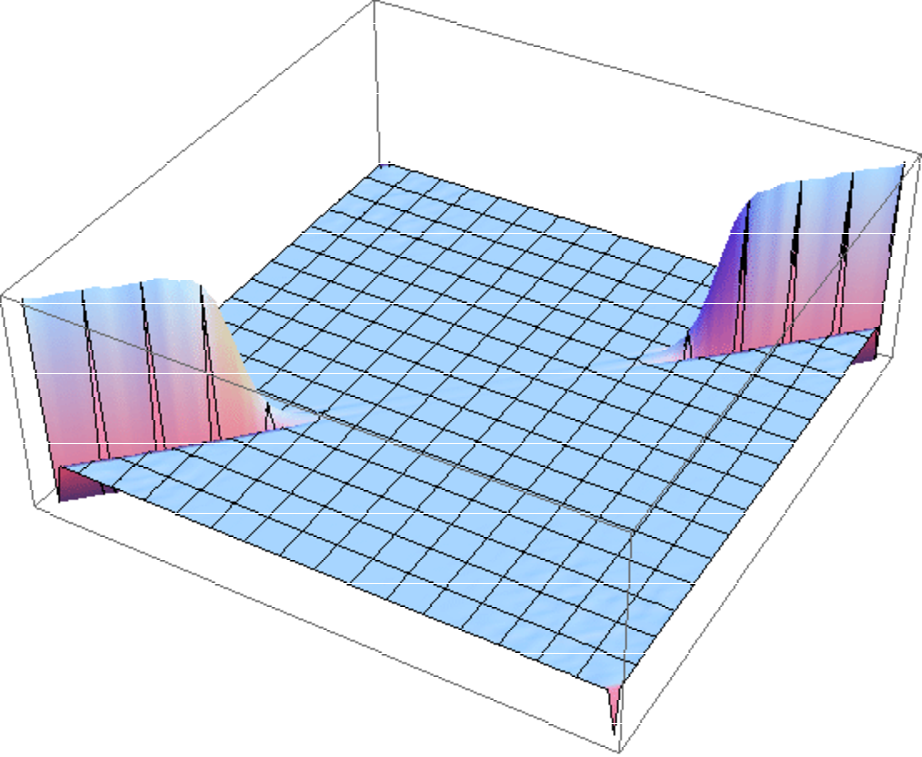
The tridiagonal form suggests that the effective action describing fluctuations of is quasi-local in time,
| (4.4) |
The function describes the kinetic part of the effective action. It couples volumes of successive slices providing the non-zero subdiagonal elements of . Because both and are symmetric matrices, the function has to be symmetric in its arguments, . The potential part is described by function which contributes only to the diagonal. According to the expansion of the effective action (4.2) the elements of the Sturm-Liouville matrix are given by
where
Discrete minisuperspace action. In the next Sections, we determine functions and , and show that the effective action (4.4) corresponds to a discretization of the minisuperspace action (3.9) up to an overall sign. Below we derive a discrete version of the minisuperspace action with reversed sign
| (4.9) |
which later will be compared to the empirical action. We have incorporated the factor into constants and . The discretization procedure is not unique, but up to the order considered here, all discretizations are equivalent. We substitute the physical volume with the discrete volume , which as stated in Section 3.1 may be treated as a continuous variable inside the blob. The stalk region is governed by very strong lattice artifacts, and therefore is not reliably treated in the semiclassical approximation. The standard discretization of the time derivative is , and the kinetic part is written as
while the potential part as
Therefore, a discretized, dimensionless version of (4.9) is given by
| (4.10) |
which corresponds to
| (4.11) |
Further we show that the discrete effective action (4.10) describes not only the average (3.4), what follows from the classical trajectory of equation (4.9), but indeed also the measured fluctuations .
4.1 Decomposition of the Sturm-Liouville matrix
From the formula (4.4) follows that Sturm-Liouville operator decomposes into the kinetic part , given by the function , and the potential part , given by the function ,
Only the kinetic part contributes to the sub-diagonal elements
of the tridiagonal matrix (cf. (4)).
We make following assumptions about :
It should be a tridiagonal matrix. The square of the time derivative should couple with the preceding and following time steps.
It should be a symmetric matrix. Covariance matrix is symmetric, and so should be .
The sum of elements in each row or column should be zero.
A constant vector should be a zero mode eigenvector as it is invariant under time translations.
Taking into account time-periodicity, this implies a following form of ,
| (4.12) |
The matrix can be decomposed into parts linearly dependent on :
| (4.13) |
where is a matrix corresponding to the discretization of the second time derivative at a time ,
In the case of the potential term, we have to get rid of the zero mode. The measured potential is a projection of the potential part of the full, unconstrained inverse propagator on a subspace orthogonal to . Assuming that the full potential matrix is diagonal
and following equation (B.3) derived in the Appendix B, we get the empirical propagator inverse
| (4.14) |
which can be decomposed into linear combination of matrices
Here, denotes the unit matrix. The kinetic part remains unaffected by the projection, since .

The decomposition of the empirical matrix into a kinetic and potential part, is done using the least square method. We find such values of and , for which the matrix , given by (4.13) and (4.14), is as close as possible to the empirical matrix , i.e. we minimize the residual sum of squares
| (4.15) |
We will omit details of the parameter fitting. In fact, we used the weighted least square method, giving higher weights to slices with larger volumes, i.e. lying inside the blob. Equation (4.15) is quadratic in and , and the fitting boils down to calculating traces of products of matrices and .
4.2 Kinetic term

In this Section we show that the fitted values of the kinetic term , obtained by minimizing residues (4.15), are indeed in agreement with the kinetic part of the discrete minisuperspace action (4.10). For the minisuperspace model, equations (4) and (4.11) give
| (4.16) |
and in the zeroth order approximation, , we have following behavior of the kinetic term
| (4.17) |
Fig. 4.3 presents the plot of for the empirical values of and various total volumes . The theoretical fit (4.17) agrees extremely well with the measured quantities. Additionally, the effective coupling constant does not depend on in the margin of error. For , we measured . The kinetic part of quantum fluctuations is indeed described by the minisuperspace action (4.9).
This success in applying the minisuperspace model to Causal Dynamical Triangulations in four-dimensions, encourages us to check if we can say something about the potential term making use of the knowledge only about the kinetic part and the classical trajectory. The classical solution minimizes the action,
Assuming that the minisuperspace model is valid, after inserting the function given by (4.11) into the action (4.4) we get an equation for the first derivative of the potential for arguments equal to the average spatial volumes,
Fig. 4.4 presents the evaluated derivative of the potential, for empirical values of average spatial volume . Again, the measurements agree within the limit of error with the prediction (4.11)
4.3 Potential term

In this Section we directly show that values of the potential term extracted from the empirical inverse propagator also agree with the minisuperspace model. Within this framework, following equations (4) and (4.11), we expect that
| (4.18) |
Fig. 4.5 shows the measured values of coefficients extracted from the empirical matrix . Because of large statistical errors, it is not an easy task to determine . As can be seen in Fig. 4.5 the plot is dominated by the stalk which is governed by lattice artifacts and can not be reliably treated semiclassically. The physically interesting region of large volumes corresponds to relatively small values of as they are expected to falls as . Due to the projection on the space orthogonal to the zero mode, the blob region is affected by the huge contribution from the stalk. Moreover, analogically as in the ordinary path-integral approach to quantum mechanics when the time step approaches zero, in the continuum limit the potential term is sub-dominant w.r.t. the kinetic term for individual spacetime histories in the path integral.

Nevertheless, due to sufficiently long Monte Carlo sample, the obtained results allowed us to confirm that indeed the formula (4.18) is in agreement with the measurement. Fig. 4.6 presents the measured coefficients as a function of the average three-volume . The error bars shown on the plot, were estimated using Jackknife method. Such a form allows us to directly compare the potential coefficients with theoretical predictions . The selected range of corresponds to the bulk, and is highlighted in Fig. 4.5. The best fit of the form to the empirical values as a function of gives . The measured exponent coefficient is very close to the theoretical value . The fit , corresponding to the potential (4.11) is presented in Fig. 4.6 with a thin line. The agreement with the data is good, the potential part of the effective action is indeed given by . There is a very small residual constant term present in this fit, which presumably is due to the projection onto the space orthogonal to the zero mode. In view of the fact that its value is quite close to the noise level with our present statistics, we have simply chosen to ignore it in the remaining discussion. Apart from obtaining the correct power , the coefficient in front of this term is also independent of .
In summary, we conclude that the measurements of the covariance matrix of quantum volume fluctuations allowed us to reconstruct the discrete version of the minisuperspace action (4.10) with a high precision.
4.4 Flow of the gravitational constant
In the previous Section we gave a direct numerical evidence that quantum fluctuations of three-volume are very accurately described by the discrete, dimensionless effective action
| (4.19) |
where we omitted the cosmological constant term since during the measurements the total volume was fixed. This action comes out as a discretization of the minisuperspace action (3.9) with the opposite sign which solves the problem of unboundedness. Let us note, that it is justified to use the semiclassical approximation as the distribution of spatial volumes in the bulk (cf. Fig. 3.2) is given by Gaussian fluctuations around the mean.
In this Section we establish the relationship between the discrete action (4.19) and its continuum counterpart (3.9), which will allow us to connect the effective coupling constant with the gravitational constant coupling constant . At first, let us rewrite the above action in terms of the normalized volume . Using equations (3.12) and (3.11), where , the discrete action can be written as
and following (3.13), we can represent it in a form of an integral over the continuum time
| (4.20) |
As stated in the previous Sections the effective coupling constant does not depend on when the bare coupling constants are fixed, the same is true for the classical trajectory . Hence, the amplitude of fluctuations of scales with the total discrete volume as and they vanish in the continuum limit , while the background stays fixed. Regarding Fig. 3.4, it means that the height of the curve will grow as , but the superimposed fluctuations will only grow as , and for fixed bare coupling constants the relative size of fluctuations will go to zero in the infinite-volume limit. Therefore, in order to obtain a proper continuum limit with a finite physical four-volume and finite fluctuations (cf. (3.20)), one also has to properly tune the bare coupling constants so that the effective coupling constant satisfies while taking and .
Further, we rewrite the action (4.20) in terms of the physical volume . Using formulas (3.19) and (3.20), we recover a continuum action back from the discrete action (4.19)
| (4.21) |

This is the second most important result obtained in this dissertation. Not only the average spatial volume obtained in the Causal Dynamical Triangulations frameworks is given by the classical trajectory of the minisuperspace model, but also the fluctuations of around the background geometry are described by the minisuperspace model up to the overall sign.
It is natural to identify the coupling constant multiplying the effective action for the scale factor (3.9) with the Newton’s gravitational constant . The effective action describing our computer-generated data (4.21) can be directly compared with the minisuperspace action (3.9), and using equations (3.21) and (3.22), we get following relations between the gravitational constant and the effective constant [45, 46],
| (4.22) |
This result is consistent with our earlier conclusion, in order to keep the physical constant fixed, when taking the continuum limit one has to tune the effective coupling constant . This means that in terms of the lattice volume fluctuations should diverge, and this happens when we approach a second or higher-order transition line. Therefore it is important to determine the order of transition. If the - transition would be of the first-order we may hope that the triple point is of higher order, which is often true, and obtain the proper continuum limit while approaching this point. Fig. 4.7 shows the measured effective coupling constant for various values of . Indeed when we approach the - transition line tends to zero. However, it is not so easy to find the exact path in coupling constant plane, as formula (4.22) depends also on other parameters, namely the effective four-volume shared by one spatial tetrahedron and the width of the distribution , and it will require further extensive computer-experiments.
The Universe size. Using relation (4.22) we can express the cut-off length in terms of the Planck length, and thus estimate the size of the Universe generated in computer simulations. Let us recall that in natural units . For the bare coupling constants we measured the quantities: , which results in and the linear size of the universe built from simplices is about . The quantum de Sitter universes studied here are therefore quite small, and quantum fluctuations around their average shape are large (cf. (3.4)). Surprisingly, the semiclassical minisuperspace formulation gives an adequate description of the measured data, at least for the volume profile.
To conclude, based on the numerical evidence we reconstructed the discrete effective action describing quantum fluctuations of the three-volume . This allowed us to identify the effective action with the discretization of the minisuperspace action with a negative sign. We also derived a relation between the physical gravitational constant and the effective coupling constants appearing in the model, giving a recipe of how to obtain a meaningful continuum limit.
Chapter 5 Geometry of spatial slices
This chapter is based on the publication:
J. Ambjørn, A. Görlich, J. Jurkiewicz and R. Loll,
”Geometry of the quantum universe”,
Phys. Lett. B 690, 420 (2010).
After investigating in Chapter 3 the four-dimensional geometry of the quantum Universe, the next step is to look deeper into the geometry of spatial slices. A spatial slice is a leaf of the imposed global proper-time foliation and is labeled by a discrete time index . Each slice is built of equilateral spatial tetrahedra. A hypersurface of this kind is a three-dimensional triangulation, more precisely, a piecewise linear manifold of topology . However, it does not mean that the geometry of slices is close to the geometry of a three-dimensional sphere.
5.1 Hausdorff dimension
Since in this Chapter we consider each slice as a separate object, let us denote the number of tetrahedra building a slice by the discrete three-volume . A basic observable defined on a slice, is the number of tetrahedra at a three-dimensional distance from some initial tetrahedron . A three-dimensional distance is based on the definition of tetrahedra neighborhood within one slice, while a four-dimensional distance is based on the definition of simplices neighborhood (cf. Section 3.4). This difference introduces a significant change in the shell decomposition picture. At distance only the initial tetrahedron is counted and . Next, we move out by one step visiting all four neighbors of , thus . Moving out by a further step, there will be tetrahedra at a distance , and so on until all tetrahedra are visited, with the restriction that one tetrahedron is visited only once. For such definition, corresponds to an area of the shell of radius . Summing up the area over all shells gives the discrete volume of a slice ,
Further, denotes the average of over all initial tetrahedra ,
In this Section we investigate scaling properties of with respect to the slice volume .

The Hausdorff dimension of spatial slices may be measured, using the scaling properties, in a following way [30]. For a given slice of volume , we define the average linear extent as
For each slice we obtain a data pair . Such pairs are then gathered for all slices of a number of Monte Carlo (MC) configurations. A plot off all points belonging to some MC sample, shown in Fig. 5.1 for , looks like a cloud. To make the average behavior more visible, the number of data points is reduced. The results are sorted by and averaged over a sequence of consecutive points (in contrary to [30] where the sample is sorted by , because fluctuations of are larger than , the approach used here gives smaller finite size effects and better linear behavior of the log-log plot.) For Hausdorff dimension , the expected relation between the slice volume and the average linear extent is following
| (5.1) |
The reduced data points (green dots) together with the relation (5.1) fitted to the full data are presented in Fig. 5.1. The fitted value of the Hausdorff dimension is .

Similar results can be obtained by a direct comparison of the scaled with volume values of the radial volume . First, for a large number of Monte Carlo configurations, slices with the same volume (more or less few tetrahedra) are collected into groups. The average radial volume within a group is denoted as . Next, the radius and the average volume are scaled and normalized in the following way
| (5.2) |
Analogically as in Section 3.4, where we calculated the scaling dimension for (cf. Fig. 3.5 and 3.6), we define the error of the overlap of the scaled points and find such value of which minimizes the dispersion. The best fit is obtained for . Fig. 5.2 presents the measured values of scaled according to (5.2) with and for various values of between and tetrahedra.
The Hausdorff dimension may be also estimated from the small behavior of . The value determines the dependence of the volume of a ball on its radius , or equivalently for an area of a sphere
Because is interpreted as the area of a sphere with a radius , the expected behavior of for small is . Assuming that for small , is the only exponent consistent with the scaling (5.2). Fig. 5.2 shows that is in agreement with the measured data. This method of estimating the Hausdorff dimension, is however more sensitive on the fit region than studying the scaling properties.
To conclude, all methods of determining the Hausdorff dimension of spatial slices give consistent results. The measured value is with a high accuracy equal to . Moreover, the measured value of is independent of the coupling constants and , as long as we stay well inside the phase . This results is true if we consider the ensemble average of the slice geometry. As we shall see in the next Sections, this result does not mean that individual spatial slices resemble a smooth three-dimensional geometry.
5.2 Spectral dimension
In this Section we determine spectral dimension by investigating diffusion process on triangulated slices dominating in the CDT partition function in phase . We measure the spectral dimension in the same way as described in Section 3.4. The probability of finding a diffusing particle in tetrahedron after a diffusion time and starting at tetrahedron is given by the probability density . The discrete diffusion equation, describing the evolution of the probability density, is an analogue of the equation (3.26), namely
| (5.3) |
where the sum is over all tetrahedra adjacent to . For a starting tetrahedron , chosen at random, we set the initial condition . By iterating the diffusion equation, we calculate the return probability for successive discrete diffusion steps . Further, we compute the average return probability by averaging over initial points and configurations. For each configuration we consider only the central slice. Spectral dimension is obtained from the return probability using the definition (3.25)
| (5.4) |
In the case of Euclidean space , the spectral dimension and Hausdorff dimension are equal to the topological dimension . For a three-sphere , spectral dimension is equal for short diffusion times. Because of the finite volume, for longer times the zero mode of the Laplacian will dominate and will tend to zero.

Fig. 5.3 shows values of the spectral dimension as a function of the diffusion time determined by numerical simulation using the definition (5.4) for a randomly chosen typical configurations in phase C. Due to the discrete lattice structure, for small values of a split for even and odd diffusion times is observed. Because of finite volumes of slices, for very large , falls down to zero. For the intermediate region, there is a plateau of the spectral dimension at .
5.3 The fractal structure of spatial slices
The measured value of the spectral dimension of spatial slices is significantly smaller than the Hausdorff dimension . The difference between and is an indication of a fractal nature of slices. We will now identify this fractal structure in a more direct way. Three-dimensional spatial slices demonstrate a very similar structure to triangulated universes present in three-dimensional Euclidean Dynamical Triangulations (EDT). It is known, that in three-dimensional EDT so-called baby Universes separated by minimal necks are observed [64, 65]. Advocated by the presence of such objects in the Euclidean theory, we look for their existence inside spatial slices.

A minimal neck denotes a set of exactly four triangles forming a tetrahedron (i.e. each triangle is connected to each other), which is not present in the triangulation. It corresponds to the smallest nontrivial boundary of a three-dimensional simplicial manifold built of tetrahedra. The minimal necks provide the three-dimensional triangulation with a tree-structure. A simplicial manifold cut along a minimal neck, by removing connections between tetrahedra which share the triangular faces belonging to the minimal neck, is decomposed into two disconnected parts. The two components form a simplicial manifold with a boundary and both of them contain more than one tetrahedron (in fact at least four). By closing the boundaries with tetrahedra we make the manifolds into two triangulation of a topology . Fig. 5.4 illustrates a minimal neck in the case of a two-dimensional triangulation. In two-dimensions a minimal neck is created of three links forming a missing triangle and is drawn with a thick black line, it separates the triangulation into a blue and red part.
It is natural to visualize this structure in the form of a tree graph. The procedure of creating such tree is following:
- •
We find all minimal necks, i.e. sets of four triangles forming a tetrahedron which does not belong to the triangulation.
- •
Each triangle is a common face of two tetrahedra. Ungluing the tetrahedra sharing elements of a minimal neck decomposes the triangulation into two parts.
- •
We cut the triangulation along all minimal necks, separating the slice into many disconnected pieces. We represent each piece as a vertex. To each vertex, we can assign the number of tetrahedra building a corresponding piece. This number is called a vertex volume.
- •
We add an edge linking two vertices if they share a common minimal neck. Because the slice has a topology of a three-sphere, by definition the set of vertices and edges forms a connected tree graph, called a minbu tree.


Fig. 5.5 presents two minbu trees created by the above procedure and corresponding to two randomly chosen successive slices. Considering one graph, we see that it is indeed a tree, but what is most important it has a fractal structure (regarding for finiteness). Very often, but at random places, a branch bifurcates into two or more branches. Most probably, when the size of the slice grows to infinity, one would observe a real fractal structure of an infinite branched polymer.
The definition of a minbu tree gives very similar results as the definition of diffusion trees used in case of spatial slices (cf. Section 3.4). The full four-dimensional geometries did not exhibit any fractality, four-dimensional analogues of minimal necks appeared very seldom. In contrast, if we had created a diffusion tree for a spatial slice, we would observe the same fractal structure as presented in Fig. 5.5, with even more bifurcation points. The advantage of a minbu tree is that it does not introduce any specified initial tetrahedra. The graph in Fig. 5.5 is centered on the edge which divides the tree into two most equal parts with respect to the three-volume.
The fractal structure suggest that leaves of the imposed time foliation have no semiclassical meaning. One has to perform an average of observables over all triangulations as we did in previous Sections. On the other hand, we checked that three-dimensional distance hierarchy reflected by the minbu tree (every path connecting two tetrahedra in different vertices must cross the appropriate minimal necks), is not an artifact of the imposed foliation and persist in the full, four-dimensional embedding. There are no drastic shortcuts through the four-dimensional simplicial complex.
This is corroborated by studying if the fractal structure survives between one time slice and the next. Fig. 5.5 illustrates minbu trees for two consecutive slices and . Using the full four-dimensional triangulation, we introduce the notion of neighbors on vertices of two trees. A vertex of a tree is a neighbor of the vertex of a tree , if there exists a pair of tetrahedra respectively shared by each vertex between which four-dimensional distance is , i.e. the shortest path between two slices passing through simplices , , and finally . Intuitively this means that two vertices are as close as possible in the four-dimensional simplicial manifold. One vertex may have many neighbors and the relation is symmetric. This notion allows us to study if the tree structure propagates over successive slices, i.e. if it survives from one slice to the next or if there is no correlation. For purposes of illustration, as shown in Fig. 5.5, we have marked all vertices of a given tree branch at time in a chosen color. For each vertex we then find its neighboring vertices in time slice , and mark them with the same color, allowing also for mixing of colors. Clearly one can explicitly identify branches in the two slices, which proves that the fractal structure is correlated and not totally independent of each other. Nevertheless, the branches may significantly change their shape. The relation with further slices decays fast as the time step separation grows. So far, we have only this qualitative notion at our disposal. It is a challenge to define more quantitative methods measuring the correlation of successive trees, i.e. an analog of scalar product acting in the space of trees based on a four-dimensional definition of distance.
We conclude that the measurements of Hausdorff dimension evidently show that . The spectral dimension is equal only half of this value, . Such behavior indicates that the geometry of spatial slices is completely different from a smooth geometry of a three-sphere. Indeed, direct measurements on individual slices prove that they are equipped with a fractal structure similar to branched polymers. Quantum fluctuations can not be described by small Gaussian fluctuations around some average geometry, suggesting that the specified hypersurfaces of constant time are not physical. Still, the tree structure propagates over consecutive slices.
Chapter 6 Implementation
The main tool used to obtain results within the framework of four-dimensional Causal Dynamical Triangulations are numerical Monte Carlo simulations. In CDT the partition function (1.2) is regularized by a discrete sum (1.9) over causal triangulations . Such approach allows to generate Monte Carlo triangulations and calculate expectation values of observables according to (1.10). Therefore, we need to handle elements of the set of labeled causal triangulations . In this Chapter we introduce software solutions and data structures used to store information about objects describing a triangulation. Later, we describe details of the implementation of the Monte Carlo algorithm, especially the Monte Carlo moves.
Experience has shown that simulations are limited mainly by the available CPU time, rather than by the amount of the used memory. Therefore, the implementation of the algorithm uses a maximal information philosophy. The program stores in memory a full information about points, links, triangles and simplices. This approach allows for quicker access to the needed information at the expense of the increased memory demand.
All results presented in this work were obtained using a computer program written in C. Therefore, we use the C language syntax to describe data structures.
6.1 Parametrization of the manifold
To perform the average (1.10) the Monte Carlo algorithm has to generate configurations according to the probability distribution on an ensemble of causal triangulations . We have to define the way we code a simplicial complex and store it in the computer memory. To increase the acceptance of Monte Carlo moves, and thus the efficiency of the algorithm, we introduce many lists, enumerating the Lorentzian structures.
Once we have labeled vertices of a triangulation and set its topology, the simplicial complex is given by the adjacency relations between four-simplices. Four-simplices, which are also labeled, share five vertices. The connections between simplices induce the adjacency relations on all sub-simplices to which we also attach labels. Each label is an integer number between and some maximal value. A label uniquely identifies sub-simplices appearing in the triangulation, and instead of writing ”label of an object” we shall use a shortcut ”object”. The topology is ensured by construction. As we shall see, we start with a minimal configuration with the designated topology and introduce only local Monte Carlo moves which do not spoil the topology. Therefore, to perform simulations the program has to code such objects as points, edges, triangles and four-simplices. It is not necessary to store information about tetrahedra (-simplices) which if needed may be easily extracted. In this Section we describe most of the data structures used in this context.
Points
The points are labeled by a dynamical sequence of labels.
The number of all accessible point labels is denoted as nn0.
Therefore possible vertex labels are 1 ... nn0.
The number of used point labels num0 is equal to the number of vertices
in the triangulation .
Some Monte Carlo moves are possible to be realized only on a local structure
containing a point with a coordination number equal .
Coordination number of a sub-simplex is denoted as the number of four-simplices
sharing a given sub-simplex.
The list of used labels is stored in the array list0 which has a following structure:
- •
Positions
1 ... num0are the used labels:- –
Positions
1 ... num80are the labels of points with coordination 8 (used in move ). - –
Positions
num80 + 1 ... num0are the rest of used (labels of) points.
- –
- •
Positions
num0 + 1 ... nn0are the unused labels.
The properties of all points are stored in the array p indexed by integer point labels:
point p[nn0];
The structure point (declared in the file types.h) holds information about a vertex:
typedef struct
{
    int i;      /* Index in list0                             */
    int n;      /* Coordination number                        */
    int l;      /* a random link which shares this vertex     */
    int t;      /* a random triangle which shares this vertex */
    int s;      /* a random simplex which shares this vertex  */
    int time;   /* time coordinate, number of the time slice  */
} point;
The fields of the structure point have a following interpretation:
- •
Field
icontains index of this vertex in the arraylist0,
i.e.list0[p[num].i] = num. - •
The coordination number
ndenotes the number of simplices, which share this vertex.nis not less than 8. - •
Field
lis a label of a (random, among many) link sharing this vertex. - •
Field
tis a label of a (random, among many) triangle sharing this vertex. - •
Field
sis a label of a (random, among many) simplex that shares this vertex (used in move ). - •
Field
timestores the integer time coordinate of a point, i.e. the number of a slice to which the point belongs. Two points may be connected by a link only if their time difference is not larger than one.
Links
Links are labeled by a dynamical sequence of labels.
The list of used labels is in the array list1 with a following structure,
analogical to array list0:
- •
Positions
1 ... num1are the used labels:- –
Positions
1 ... num61sare spatial links with a coordination 6 (used in move ). - –
Positions
num61s + 1 ... num61s + num41t(nextnum41t) are time links with coordination 4 (used in move ). - –
Positions
num61s + num41t + 1 ... num1are the rest of used links.
- –
- •
Positions
num1 + 1 ... nn1are the unused labels.
The data about all links are stored in array l indexed by links labels:
digon l[nn1];
The structure digon (defined in types.h) holds information about a link:
typedef struct
{
    int p[2]; /* Labels of endpoints            */
    int n;    /* Coordination number            */
    int s;    /* Simplex which shares this link */
    int i;    /* Position in list1              */
    int h;    /* Hash code of this link         */
    int n2;   /* Next link in a hash table list   */
} digon;
The meaning of the fields is as follows:
- •
The labels
pof the endpoints. The labels are sorted:p[0] < p[1]. - •
The coordination number
ndenotes the number of simplices, that share this link.nis at least for time links, and at least for spatial links. - •
Field
sis a label of one (random, among many) four-simplex containing a link with given label. - •
Field
icontains the position of the link in the arraylist1:list1[l[num].i] = num. - •
Field
hcontains the hash code for the link:l[num].h = hlc(l[num].p[0], l[num].p[0]). - •
Field
n2contains the label of the next link in the singly-linked list of links with the same hash-codeh.
Hash map
In move 2 a time link with a coordination 4 is created, while in move 5 a spatial link with coordination 5 is created. It might happen that a link with the same endpoints already exists. In this case we have to abort the move.
In order to perform a fast search of a link given the labels of its endpoints,
the hash table is used.
Knowing the labels of vertices p[0] p[1]
we calculate the hash code h using the hash function hlc
h = hlc(p[0], p[1]) = ((p[0] << 10) xor p[1])
defined in file core/hash.h.
The first element of a singly-linked list of links with the same hash code h
is given by hlt[h].
The next element in the list is accessed via the field n2 in the structure digon.
To find if a given link exists, we have to look through this list - very short on average.
Triangles
The triangles are labeled by a dynamical sequence of labels stored in the array list2:
- •
Positions
1 ... num32tare time triangles with a coordination 3 (used in move 3). There are no time triangles with coordination less than 3. - •
Positions
num32t + 1 ... num32t + num42sare spatial triangles with a coordination 4 (used in move 5). There are no spatial triangles with a coordination less than 4. - •
Positions
num32t + num42s + 1 ... num2are the rest of used links. - •
Positions
num2 + 1 ... nn2are the unused labels.
The properties of all triangles are stored in the array t indexed by a triangle label:
triangle t[nn2];
The structure triangle (declared in types.h) holds information about a triangle:
typedef struct
{
    int p[3];  /* Labels of vertices                 */
    int n;     /* Coordination number                */
    int s;     /* simplex which shares this triangle */
    int i;     /* Position in list2                  */
    int h;     /* Hash code of this triangle         */
    int n2;    /* Next triangle in hash table list   */
} triangle;
- •
Field
pstores sorted labels of vertices:p[0] < p[1] < p[2]. - •
Field
nis a coordination number of a triangle, i.e. athe number of simplices, that share this triangle. It is not less than 3. - •
Field
sis a label of a simplex which shares this triangle (used in move 3). - •
Field
icontains index of this triangle in the arraylist2. - •
Field
hcontains the hash code of a triangle:t[num].h = htc(t[num].p[0], t[num].p[0], t[num].p[2]). - •
Field
n2contains the label of the next triangle in the singly-linked list of triangles with the same hash-codeh.
Hash map
In move 3 a time triangle with a coordination 3 is created, while in move a spatial triangle with a coordination 4 is created. It might happen that this triangle already exists (a triangle with the same vertices). In this case we have to abort the move.
To perform a fast check if a triangle with given vertices exists,
a hash table is used.
Given the labels of vertices p[0] p[1] p[2]
we calculate the hash code h using the hash function htc
h = htc(p[0], p[1], p[2]) = (p[0] * 256) xor (p[1] * 16) xor p[2]
defined in a file core/hash.h.
The first element of a singly-linked list of triangles with the same hash code h
is given by htt[h].
The next element in the list is accessed via the field n2 in the structure triangle.
Similarly as for links, to find if a given triangle exists, we have to look through this list - very short on average.
Simplices
In CDT, there are two types of simplices:
- •
type and with four vertices in one time layer,
- •
type and with three vertices in one time layer.
The list of simplex labels is stored in the array list4 with a following order:
- •
Positions
1 ... num444are simplices of type and . - •
Positions
num444 + 1 ... num4are simplices of type and . - •
Positions
num4 + 1 ... nn4are the unused labels.
The properties of all simplices are stored in the array s indexed by a simplex label:
pentachoron s[nn4];
The structure pentachoron (declared in types.h) holds information about a simplex:
typedef struct
{
    int p[5];   /* Labels of vertices */
    int s[5];   /* Labels of adjacent 4-simplices */
    int l[10];  /* Labels of links shared by simplex */
    int t[10];  /* Labels of triangles shared by simplex */
    int i;      /* Position in list4 */
    int rez[5]; /* Reserved. Aligned to 32 */
} pentachoron;
The fields of the structure pentachoron store a following information:
- •
Field
pstores labels of vertices of a simplex. - •
Field
sstores labels of the neighboring simplices. Simplexs[i]is the neighbor opposite top[i]. - •
Field
lstores labels of links shared by a simplex. The links in the listlare sorted w.r.t. the first endpoint, and then w.r.t. the second one, where the ordering of the endpoints is given byp[i]. - •
Field
tstores labels of triangles shared by a simplex. The triangles sorted w.r.t. the first, second than third endpoint where the ordering of endpoints is given byp[i]. - •
Field
iis the index of a simplex in the arraylist4.
On simplices, we finish the description of the data structures used to store full information about the triangulation. The general idea of the Monte Carlo program boils down to initialize above structures and sequential calling procedures that modify data in accordance with Monte Carlo moves.
6.2 Monte Carlo Simulations
The idea behind the Monte Carlo simulations is to approximate the sum appearing in the partition function (1.9) by a sum over a finite number of Monte Carlo configurations. More precisely, given an observable , e.g. a distribution of a three-volume of spatial slices, we would like to calculate its expectation value . In the CDT framework the geometries are already restricted to a discrete set of simplicial manifolds and
| (6.1) |
where the partition function is given by eq. (1.9) with the action (1.5) and the corresponds to the labeling of .
Monte Carlo simulations generate a finite set of configurations and allow to approximate the average (6.1) by a summation over it,
| (6.2) |
Let us notice, that no factor is needed, since configurations are generated according to the probability distribution , which means that more probable geometries will more likely appear in the set . We implement the Metropolis-Hastings algorithm to generate a Markov Chain using Monte Carlo methods [67, 68]. We define and implement local transformations, called Monte Carlo moves, which modify a configuration . The Monte Carlo move applied to a triangulation transforms it into a triangulation . A series of such moves defines a Markov chain, the next configuration depends only on the last and on the applied move. After one step configurations and are almost identical, but after sufficiently large number of moves separating them, the initial and final configurations are independent. If the moves are chosen randomly, the algorithm performs a random walk in the phase-space of configurations, i.e. causal triangulations . The moves are however not chosen completely at random. The moves and their weights, i.e. probability of being realized, must fulfill some constraints in order to properly probe the ensemble of causal triangulation according to (6.1). The algorithm, after satisfying the conditions described below, ensures that it samples the configuration space according to a probability distribution
The Monte Carlo moves must fulfill following conditions:
Ergodicity.
The moves generating the Markov chain have to be ergodic.
It means that it is possible to reach any topologically equivalent
causal triangulation by a sequence of such moves.
Our scheme of assembling an appropriate set of elementary moves
is to first select moves that are ergodic within the spatial slices.
This is clearly a necessary condition for ergodicity in the full triangulations.
Namely, those are moves and together with their inverse moves
11
1
The numeration of moves corresponds to the convention used in the computer program..
These moves act on spatial slices like
three-dimensional Pachner moves
which are equivalent to the primal Alexander moves
and thus proved to be ergodic and preserving the topology of the space [70, 69, 71].
Then we supplement them by moves and acting within two spatial slices. They do not affect connections between tetrahedra building the spatial slices and can be understood as a Lorentzian variant, i.e. combination, of the four-dimensional Pachner moves, in the sense that they are compatible with the discrete time slicing of our causal geometries [29, 47]. The moves are described in detail in the next Section.
Topology and causality. Because move is self-dual, the CDT program is using a set of seven local moves, being a combination of Pachner moves. By construction, these moves do not destroy the topology of the spacetime, and preserve the global proper-time foliation. Moves affecting the spatial slices preserve the topology of the space. The two features define the entropy factor. In fact, we know neither what class of geometries we should consider in quantum gravity nor the proper measure. The CDT model is a trial to define these objects.
Detailed balance condition. The previous two points are independent of the probability distribution of configurations specified by the action . Given a move, it transforms a configuration into configuration . In order to ensure that the Monte Carlo algorithm probes the configuration space with probability , the move has to be accepted with some probability weight and satisfy the detailed balance condition:
This condition determines the weights, however not uniquely. The probability depends on the considered model. The transition probability is a product of two factors:
The first is determined by the way we choose a position in where the move is performed and by the move type. The second is chosen such that the detailed balance condition is satisfied. Once we have decided what Monte Carlo moves, and how we implement them, the weight is fixed and depends on the internal probability of choosing a move. A good Monte Carlo algorithm has the weights and close to . This is equivalent to a high acceptance of moves.
Autocorrelation and thermalization time. An accurate approximation of the average (6.2) requires a suitably large sample of independent configurations . Configurations are collected in intervals, measured in a number of Monte Carlo steps, whose length determine correlations between configurations. Intuitively, the larger is the number of Monte Carlo moves which separate triangulation and the more uncorrelated they are. The separation should be chosen properly based on the autocorrelation time, which can be estimated using some slowly changing variables, like a width of the volume distribution or its mass center position. We will refrain from discussing the details of this numerical procedure. Before we can start measurements, the configurations have to undergo a thermalisation procedure, which consists on sufficiently long execution of the algorithm without performing measurements.
Tuning of .
The Regge action (1.5) depends on three bare coupling constants and .
For technical reasons of simulations it is preferable to enforce that the total number
of four-simplices fluctuates around some prescribed value nvolume
during the Monte Carlo simulation.
The coupling constant is related to the bare cosmological
coupling constant.
If the value of is smaller than its critical value ,
the total volume tends to explode.
In the opposite case , the configuration collapses.
Thus should be tuned to its critical value.
In practice we use a modified Regge action by adding a term
which, for , ensures that fluctuates around nvolume.
Alternatively, we can add a quadratic term
which is also studied. Presented results are consistent in both cases.

Starting configurations. Before we can apply the moves and generate a Markov chain we must create the initial configuration. We construct a minimal configuration with a topology . Fig. 6.1 presents a two-dimensional analogue of the starting configuration. First, we assemble the simplest three-dimensional simplicial complex with a topology , corresponding to a spatial slice at a fixed time. It is a boundary of a 4-simplex and contains five tetrahedra glued to each other. Let us label five vertices of this complex by . Then the five tetrahedral interfaces are denoted as
Next, we take two such structures, first at time with vertices , second at time with vertices . And join them with a minimal number of 4-simplices. Each of five interfaces at time becomes a base of a simplex with a top vertex at time , thus creating five four-simplices. Let us denote these by
These are supplemented by 10 simplices of the type :
Likewise, mirror reflected simplices are created, 10 simplices of the type :
and finally 5 simplices of the type :
The result of these operations is a four-dimensional segment with a topology . In total, one segment is composed of five simplices of type , ten simplices of type , ten simplices of type and five simplices of type summing up to 30 simplices. The boundary of a segment consists of two identical components, built of five interfaces. A number of segments can be iteratively joined one after another forming a simplicial manifold of a desired time length. In order to obtain a starting configuration with a topology , i.e. periodic boundary conditions, the interfaces at the beginning and at the end are glued together.
Algorithm
The scheme of the algorithm is as follows:
- 1.
We select the type of a move at random. The probabilities are chosen in such a way that the numbers of accepted moves of each type are approximately the same.
- 2.
Each move type is related to a characteristic structure of simplices, which must be met in order to be accepted. We choose at random a point, link, triangle or simplex that satisfy these conditions. The design of the program provides a quick access to such elements.
- 3.
We check if the new simplicial complex corresponds to a triangulation of a manifold. One must avoid creating simplices or subsimplices already present in the triangulation. Also, the move must not destroy the foliation.
- 4.
We compute the Metropolis weights and accept or reject the move with proper probabilities.
- 5.
We update the lattice structures.
In the next Section we describe all types of moves, in particular we describe the conditions which must be satisfied in order to perform a move.
6.3 Monte Carlo Moves
We start the discussion of Monte Carlo moves with recalling
the Regge action which determines the probability distribution (6.1)
on the ensemble of causal triangulations.
The implementation of moves may be found in files moves/move??.c (?? denotes a particular move name).
The action used in the program is parametrized as:
where , and are bare coupling constants and is the number of vertices, is the number of simplices, is the number of simplices of the type . In the remaining part of this Section we focus on particular types of moves.
Move 2
Move replaces the interface between the two four-simplices by a link dual to the interface. Here the numbers denote labels of vertices involved in the move, and the bracket denotes a tetrahedron built on given vertices. The new link has a coordination number . We can only create a new time (and not space) link with a coordination 4. This can easily be checked before the move is attempted. The first step in the move is to pick a or four-simplex from the list and to chose the interface. The neighboring four-simplex can be either again a or four-simplex or a or four-simplex. The move is accepted with a different weight in these two cases, since in the first case there are two ways it can be realized and in the second only one way, this affects . The operation of the move can by schematically written as
The effect of this move is:
- •
The number of points does not change. .
- •
New time link with coordination number is created.
- •
Four new time triangles with a coordination number are created.
- •
Two simplices of type are created. , .
The weight for the move depends on the Regge action and is given by
where denotes a triangulation before performing the move and after performing the move. This relation determines the value of .
Move
It is an inverse of move 2. It requires a (time) link with a coordination number 4. Its action can be summarized by
- •
The number of points does not change. .
- •
Time link with a coordination number is removed.
- •
Four time triangles with a coordination number are removed.
- •
Two simplices of type are removed. , .
Analogically as in previous move, the weight for the move is .
Move 3
A self-dual move. It requires a time triangle with a coordination number 3, and replaces it by a dual triangle with the same coordination number. A triangle with a coordination 3 can only be a time triangle. The spatial triangles necessarily have coordination 4 or more. It can be easily seen by a following argument: a spatial triangle is an interface between two spatial tetrahedra. Therefore it will belong to at least 4 four-simplices, for which these tetrahedra are bases and the tips point up or down. In other words creating spatial triangles with a coordination 3, although superficially possible, creates a topological defect.
- •
No new points nor links are created. .
- •
Triangle is removed.
Triangle is created. - •
The number of simplices does not change. .
All changes are zero, the weight is .
Move 4
This move adds a new vertex at a given time slice . It acts on a configuration of and simplices. Let the two simplices be and , where bars indicate the time position of points. We produce a new point between the two simplices. The move adds 6 new simplices of type to our system, and the vertex has a coordination number equal .
- •
One new point with a coordination number is created.
This property is used as a signal for the inverse move. . - •
Four new spatial links with a coordination number are created.
Two new time links with a coordination number are created. - •
Six new spatial triangles with coordination number are created.
Eight new time triangles with a coordination number are created. - •
Six new simplices of the type are created , .
The weight for this move is .
Move
This move is an inverse of move 4. We pick point with a coordination 8 from the list of vertex labels. Such a point may be shared only by simplices of type and the neighborhood satisfies the necessary constraints. In this move the spatial interface is created and we have to check if such interface does not already exist. If yes, we abort the move.
- •
Point with a coordination is removed.
- •
Four spatial links with a coordination are removed.
Two time links with a coordination are removed. - •
Six spatial triangles with a coordination are removed.
Eight time triangles with a coordination are removed . - •
Six simplices of the type are removed. , .
The weight for this move is
Move 5
This move consists on a restructuring of the triangle between four simplices. This move requires a spatial triangle with coordination 4. By construction it is shared by four simplices of the type . Vertices have the same time position. Vertex is in the previous layer and vertex is in the next layer (or reversed). A starting configuration must have 4 four-simplices in the following setup:
- •
The number of points doesn’t change. .
- •
One new spatial link with coordination is created.
This property is used as a signal for the inverse move. - •
Two new time triangles with a coordination are created.
Three new spatial triangles with a coordination are created.
Spatial triangle with a coordination is removed. - •
Two new simplices of the type are created. , .
The weight for the move is .
Move
This move is an inverse of move 5. We pick a spatial link with a coordination 6. Such a link is always shared by simplices of the type .
- •
The number of points doesn’t change. .
- •
Spatial link with a coordination is removed.
- •
Move creates a spatial triangle with coordination , unless it already exists. If this is the case, the move is aborted. This property is used as a signal for the move 5.
Two time triangles with a coordination are removed.
Three spatial triangles with a coordination are removed. - •
Two simplices of the type are removed. , .
The weight for the move is
At this point we finish the description of the implementation of the Monte Carlo algorithm. We presented the basics necessary to create a program generating Monte Carlo configurations in the framework of four-dimensional Causal Dynamical Triangulations. A more detailed and technical description is beyond the scope of this thesis. We shall omit e.g. issues of the random number generator, preliminary acceptance, features specific to causal triangulations which allow to reject a move at the initial stage, and other solutions affecting the efficiency of the implementation.
Although we have devoted only one Chapter to the problem of the causal triangulations generator, it should be noted that the software development was the major part of the work described in this dissertation.
A copy of the source code together with the user guide and the documentation
is attached to this dissertation.
The author distributes this package on request through the e-mail: atg@th.if.uj.edu.pl
Conclusions
The aim of this thesis is to present a comprehensive review of recent results obtained within the framework of the four-dimensional model of Causal Dynamical Triangulations (CDT). We provided answers to questions like: how does a background geometry emerge dynamically, what does it correspond to and how to describe quantum fluctuations around the average geometry.
The model of Causal Dynamical Triangulations is a non-perturbative and background independent approach to quantum gravity. The foundations of this model are very simple. It is a mundane lattice field theory with a piecewise linear manifold serving as a regularization of general relativity. The introduction of Wick rotation allows to use very powerful Monte Carlo techniques and calculate quantum expectation values of observables.
Based on the Monte Carlo measurements the CDT model predicts the existence of three phases. Introduction of a qualitative order parameter describing typical geometries appearing in a given phase, allows to make a one-to-one correspondence with three phases of an anisotropic theory of a Lifshitz scalar, being an inspiration for Hořava-Lifshitz gravity model. This two models, in addition to formal similarities involving the imposition of a global time-foliation, exhibit the same scale dependence of the spectral dimension. From a physical viewpoint, particularly interesting is the phase in which the scale factor as a function of time behaves as a bell-shaped distribution spontaneously breaking the time-translational symmetry. This phase is called de Sitter phase.
In order to calculate a meaningful average of the three-volume we took into account the nonuniform volume distribution and introduced the procedure which breaks the time-translational freedom. This step was crucial to evaluate the average scale factor distribution and confirmed that a background geometry emerges dynamically. The average geometry behaves like a well-defined four-dimensional manifold, both the Hausdorff dimension and spectral dimension equal at large scales. We showed that the background geometry corresponds to a Euclidean de Sitter space, i.e. a four-sphere, an isotropic and homogeneous solution of the vacuum Einstein field equations with a positive cosmological constant. Therefore CDT produces a picture of the Universe with superimposed finite quantum fluctuations around the classical trajectory. In terms of the lattice spacing, configurations resemble a four-dimension spheroid elongated in the time direction.
The elimination of a translational mode enables to observe the emergence of the background geometry, but as a consequence also allows to investigate quantum fluctuations around the average geometry. Using Monte Carlo methods we measured the covariance matrix of scale factor fluctuations. Applying the semiclassical expansion we reconstructed the effective discrete action describing the three-volume. In the CDT model no reduction of degrees of freedom is introduced. The three-volume distribution is obtained by integrating out all degrees of freedom except the scale factor. The semiclassical expansion takes into account both the path integral measure and the bare action, making the analysis truly non-perturbative. The extracted effective action may be identified with the discretization of the minisuperspace action with an opposite sign. The effect of the reversed sign is a consequence of the entropy factor. Due to the identification, the effective coupling constant can be related to the physical gravitational constant, giving a recipe of how to obtain a meaningful continuum limit and expressing the lattice constant in terms of physical units.
Understanding of the geometric nature of three-dimensional spatial slices, interpreted as leaves of the imposed global proper-time foliation, may be of crucial importance also for other attempts to quantize gravity. Although the measurements show that the Hausdorff dimension is equal , the measured spectral dimension is only half of this value, suggesting a fractal structure of spatial slices. Indeed, the fractality is confirmed by a direct analysis of tree structures defined in terms of so-called minimal necks.
Outlook. There are many unresolved questions. The author would like to list few points he finds most interesting:
- •
What is the role of simplices of type and in better understanding of the critical behavior when approaching the phase transition?
- •
What is the order of - phase transition and how to obtain a proper continuum limit?
- •
Whether the Hořava-Lifshitz scenario is realized in our model, i.e. if the anisotropic space-time scaling in the UV-limit is observed?
- •
How to improve the Monte Carlo algorithm to increase its efficiency near the phase transition?
A physically relevant theory must describe matter fields. The work on incorporating multiple massive scalar fields and massive point particle is already in progress. We developed an efficient method of calculating field propagator on a random lattice based on a diffusion process. An important question is
- •
How to observe gravitational interaction between matter in our model and how to establish the relation between the effective coupling constant and the conventional Newton’s gravitational constant?
Appendix A Derivation of the Regge action
In this Appendix we derive the Euclidean version of the Regge action which, together with the introduced measure, defines the partition function (1.9) of the model of Causal Dynamical Triangulations. For simplicity, we start directly with the Einstein-Hilbert action (1.1) after performing a Wick rotation of the spacetime to the Euclidean region with the metric signature . The simplices building piecewise linear manifolds are embedded in the Euclidean space . Simplices are illustrated in Fig. 1.2. At the end we show that the derived action is indeed obtained by a Wick rotation of the Lorentzian Regge action. The Euclidean Einstein-Hilbert action is given by [37, 38]
| (A.1) |
where , . The Regge action is obtained by a direct evaluation of the Einstein-Hilbert action at a piecewise linear triangulation. It is straightforward to calculate that part of the action which depends on the cosmological constant, as it is proportional to the total four-volume. It is given by a sum of contributions coming from all individual simplices. We distinguish two types of simplices, namely and . Properties of all simplices within one type are identical and their geometry is completely determined by the lengths and . The total volume is therefore given by
| (A.2) |
where is the number of simplices of the type , which have a volume , and is the number of simplices of the type , which have a volume . Integration of the scalar curvature requires some attention. The curvature is singular and localized at hinges (triangles). It occurs that, in the case of triangulations, it can be simply expressed in terms of deficit angles around those hinges. Let us illustrate this on a two-dimensional example. In this case, the scalar curvature is a distribution with a support on vertices, and the angle deficit is calculated around them. A triangulation consisting of equilateral triangles sharing one vertex and periodically connected along sides may be drawn on a plane . Because the plane is flat, so is the vicinity of the common point. The sum of angles adjoint to this point equals , the angle deficit and scalar curvature vanishes. If such triangulation is built of smaller number of triangles, as shown an the top of Fig. A.1, it forms a cone and the angle deficit is positive, as is the curvature. Likewise, a larger number of triangles gathered around one vertex produces a saddle, illustrated an the bottom of Fig. A.1, with a negative curvature.

A generalization to higher dimensions was proposed by Regge in [43]. In this case besides the deficit angles the integral of the curvature depends on a volume of homogeneous hinges. It was shown that the integral over a neighborhood containing one hinge is given by
where denotes the sum of dihedral angles around the triangle and denotes its area. The integral over the whole manifold is obtained by summing contributions from all hinges. By a -triangle we will denote a triangle with vertices in one slice and in next slice. A -simplex contains two types of triangles: -triangles and -triangles. A -simplex contains -triangle, -triangles and -triangles. Each simplex shares triangles and contributes to the total dihedral angle . Using these properties we can write the global integral as
| (A.3) |
where denotes the dihedral angle between two faces of -simplex sharing a -triangle, is the triangle volume. As before all of these quantities are functions of and . The sum over all triangles equals and denotes the number of triangles of appropriate type. In order to evaluate the Euclidean Einstein-Hilbert action for a specific triangulation, one must know volumes and angles associated with simplices. Let us explicitly write down the positions of vertices of the two types of simplices embedded in the Euclidean space . We incorporate the length of spatial links into the coupling constant and rescale the edge lengths so that . The fourth coordinate defines the original time direction. The vertex coordinates of a -type simplex are:
The distances between vertices are equal , and the lengths of links ending in vertex are equal . Using these values we can calculate the simplex volume and the dihedral angle between two three-dimensional hyperplanes passing through a given triangle and respectively the two remaining vertices of the simplex
For a non-degenerate simplex we get the condition . Similarly, we find the vertex coordinates of a -type simplex. Now two vertices lie in the upper plane
Again the links lying in the same horizontal plane have the length , and the rest have . The volume of a -simplex and corresponding dihedral angles, are now given by
For a non-degenerate simplex we get the condition . The area of triangles is the same for both types of simplices and depends only on and .
To simplify equations (A.2) and (A.3) we use relations, specific for Causal Dynamical Triangulations, between numbers of appropriate sub-simplices. Despite the fact that the simplices are a subset of Euclidean space, the triangulation is equipped with the causal structure which is a consequence of the original Lorentzian spacetime and each slice is a triangulation of a three-sphere. Because each spatial tetrahedron is shared by exactly two -simplices, and those tetrahedra itself build a simplicial manifold one gets the equality between the number of spatial triangles and -simplices
Using the above equality, the Euler identity and the Dehn-Sommerville conditions for a general four-dimensional triangulation [29, 66] we get
By inserting this relation into the sum of (A.2) and (A.3), we get the Regge action for a triangulation. It is given by a very simple linear function of three independent global parameters, the number of vertices , the number of simplices and the number of -simplices,
| (A.4) |
where the coefficients, called bare coupling constants, are nontrivial functions of the coupling constants present in the continuum Einstein-Hilbert action
| (A.5) | ||||
| (A.6) | ||||
| (A.7) |
Equivalently, one can start with the Einstein-Hilbert action (1.1) and evaluate it at a Lorentzian piecewise linear manifold made up of simplices being a subset of Minkowski spacetime, as described in [29] (here we use opposite sign convention ). In the Lorentzian case is negative and the simplex volumes are given by
The same relation holds for volumes of time-like triangles. The equations for angles are identical in both cases, in the Lorentzian case angles may take complex values. Inserting the Lorentzian counterparts of volumes and angles into the Einstein-Hilbert action and taking advantage of equations (A.2) and (A.2), we get the Lorentzian Regge action. The further step is to analytically continue from negative values to positive values through the lower-half complex plane (). For the Lorentzian action becomes purely imaginary. The Euclidean action defined by relation coincides with equation (A.4).
Appendix B Constrained propagator
Let us consider a multivariate normal distribution with a component random vector and zero mean. We denote the full propagator inverse by . Further we impose a constraint on the random vector, i.e. we measure only when it is orthogonal to
For definiteness we normalized the eigenvector corresponding to the zero mode The partition function of this simple statistical model with a source term is given by
The propagator of the constrained model is given by a derivative of the constrained partition function,
In order to derive a relation between the constrained propagator and full propagator , we use the integral representation of the delta function. The function is given by
and the constrained propagator as a function of the full propagator is given by
| (B.1) |
The matrix is defined as an inverse of on a subspace orthogonal to ,
| (B.2) |
It is easy to check that
| (B.3) |
solves equation (B.2), where we used relation (B.1). The constraint inverse propagator can be expressed by the constrained propagator in the following way
| (B.4) |
From (B.1) and (B.3) it follows that and act in a space orthogonal to
Bibliography
- [1] G. ’t Hooft, M. Veltman, One loop divergencies in the theory of gravitation, Ann. Inst. Poincar´e 20, 69 (1974).
- [2] M. H. Goroff, A. Sagnotti, The ultraviolet behavior of Einstein gravity, Nucl. Phys. B 266, 709 (1986).
- [3] J. Polczynski, String Theory, Cambridge University Press (2005).
- [4] A. Ashtekar, New Variables for Classical and Quantum Gravity, Phys. Rev. Lett. 57, 2244 (1986).
- [5] A. Ashtekar and J. Lewandowski, Background independent quantum gravity: a status report, Class. Quantum Grav. 21, R53 (2004) [gr-qc/0404018].
- [6] C. Rovelli, Quantum Gravity, Cambridge University Press (2004).
- [7] A. Perez, Spin foam models for quantum gravity, Class. Quantum Grav. 20, R43 (2003) [gr-qc/0301113].
- [8] M. Bojowald, Loop Quantum Cosmology in 100 Years of Relativity. Space-Time Structure: Einstein and Beyond ed. A. Ashtekar, World Scientific, Singapore (2005) [gr-qc/0505057].
- [9] H. W. Hamber and R. M. Williams, Nonperturbative Simplicial Quantum Gravity, Phys. Lett. B 157, 368 (1985).
- [10] H. W. Hamber and R. M. Williams, Two-Dimensional Simplicial Quantum Gravity, Nucl. Phys. B 267, 482 (1986).
- [11] R.M. Williams, Recent progress in Regge calculus, Nucl. Phys. B (Proc. Suppl.) 57, 73 (1997) [gr-qc/9702006].
- [12] W. T. Tutte, A census of planar triangulations, Can. J. Math. 14, 21 (1962).
- [13] G. ’t Hooft, A planar diagram theory for strong interactions, Nucl. Phys. B 72, 461 (1974).
- [14] F. David, Planar diagrams, two-dimensional lattice gravity and surface models, Nucl. Phys. B 257, 45 (1985).
- [15] V. A. Kazakov, Bilocal regularization of models of random surfaces, Phys. Lett. B 150, 282 (1985).
- [16] J. Ambjørn, B. Durhuus, J. Fröhlich, Diseases of Triangulated Random Surface Models, and Possible Cures, Nucl. Phys. B 257, 433 (1985).
- [17] V. A. Kazakov, I. K. Kostov and A. A. Migdal, Critical properties of randomly triangulated planar random surfaces, Phys. Lett. B 157, 295 (1985).
- [18] J. Ambjørn and R. Loll, Nonperturbative Lorentzian quantum gravity, causality and topology change, Nucl.Phys. B 536, 407 (1998).
- [19] R. Nakayama, 2D Quantum Gravity in the Proper-Time Gauge, Phys.Lett. B 325, 347 (1994) [hep-th/9312158].
- [20] J. Ambjorn, J. Jurkiewicz and R. Loll, Non-perturbative 3d Lorentzian Quantum Gravity, Phys. Rev. D 64, 044011 (2001) [hep-th/0002050].
- [21] J. Ambjorn, J. Jurkiewicz, R. Loll and G. Vernizzi, 3D Lorentzian Quantum Gravity from the asymmetric ABAB matrix model, Acta Phys.Polon. B 34, 4667 (2003) 4667 [hep-th/0311072].
- [22] S. Weinberg, Ultraviolet divergences in quantum theories of gravitation in General relativity: an Einstein centenary survey ed. S. W. Hawking and W. Israel, Cambridge University Press, pp. 790-831 (1979).
- [23] H. Kawai, Y.Kitazawa, and M. Ninomiya, Renormalizability of quantum gravity near two dimensions, Nucl. Phys. B 467, 313 (1996).
- [24] M. Reuter and F. Saueressig, Functional Renormalization Group Equations, Asymptotic Safety, and Quantum Einstein Gravity, [arXiv:0708.1317].
- [25] A. Codello, R. Percacci, and C. Rahmede, Investigating the Ultraviolet Properties of Gravity with a Wilsonian Renormalization Group Equation, Annals Phys. 324, 414 (2009) [arXiv:0805.2909].
- [26] H. W. Hamber and R. M. Williams, Nonlocal effective gravitational field equations and the running of Newtons constant G, Phys. Rev. D 72, 044026 (2005) [hep-th/0507017].
- [27] J. Ambjørn and S. Varsted, Three-dimensional simplicial quantum gravity, Nucl. Phys. B 373, 557 (1992).
- [28] J. Ambjorn, J. Jurkiewicz and R. Loll, A non-perturbative Lorentzian path integral for gravity, Phys. Rev. Lett. 85, 924 (2000) [hep-th/0002050].
- [29] J. Ambjørn, J. Jurkiewicz and R. Loll, Dynamically triangulating Lorentzian quantum gravity, Nucl. Phys. B 610, 347 (2001) [hep-th/0105267].
- [30] J. Ambjørn, J. Jurkiewicz and R. Loll, Reconstructing the universe, Phys. Rev. D 72 (2005) 064014 [hep-th/0505154].
- [31] J. Ambjørn, J. Jurkiewicz and R. Loll, Spectral Dimension of the Universe , Phys. Rev. Lett. 95, 171301 (2005) [hep-th/0505113].
- [32] J. Ambjørn, J. Jurkiewicz and R. Loll, Semiclassical Universe from First Principles, Phys. Lett. B 607, 205 (2005) [hep-th/0411152].
- [33] J. Ambjørn, J. Jurkiewicz and R. Loll, Quantum gravity: the art of building spacetime, in Approaches to Quantum Gravity, ed. D. Ority Cambridge University Press (2009), [hep-th/0604212]
- [34] R.P. Feynman and A.R. Hibbs, Quantum mechanics and path integrals, McGraw-Hill, New York (1965).
- [35] H. Kleinert, Path integrals in quantum mechanics, statistics and polymer physics, World Scientific, Singapore (1994).
- [36] K. G. Wilson, Confinement of quarks, Phys. Rev. D 10, 2445 (1974)
- [37] S. W. Hawking, The Path-Integral Approach to Quantum Gravity in General relativity: an Einstein centenary survey ed. S. W. Hawking and W. Israel, Cambridge University Press (1979).
- [38] G. W. Gibbons and S. W. Hawking, Action integrals and partition functions in quantum gravity, Phys. Rev. D 15, 2752 (1977).
- [39] C. W. Misner, K. S. Thorne, J. A. Wheeler, Gravitation, W. H. Freeman and Company (1973)
- [40] R. M. Wald, General relativity, The University of Chicago Press (1984)
- [41] C. Teitelboim, Causality versus gauge invariance in quantum gravity and supergravity, Phys. Rev. Lett. 50, 705 (1983).
- [42] C. Teitelboim, The proper time gauge in quantum theory of gravitation, Phys. Rev. D 28, 297 (1983).
- [43] T. Regge, General relativity without coordinates, Nuovo Cimento 19, 558 (1961).
- [44] J. Ambjørn, B. Durhuus and T. Jonsson, Quantum Geometry, Cambridge University Press (1997).
- [45] J. Ambjørn, A. Görlich, J. Jurkiewicz and R. Loll, Planckian Birth of the Quantum de Sitter Universe, Phys. Rev. Lett. 100, 091304 (2008) [hep-th/0712.2485].
- [46] J. Ambjørn, A. Görlich, J. Jurkiewicz and R. Loll, Nonperturbative quantum de Sitter universe, Phys. Rev. D 78 (2008) 063544, [arXiv:0807.4481]
- [47] A. Görlich, Background Geometry in 4D Causal Dynamical Triangulations, Acta Phys. Pol. B 39, 3343 (2008)
- [48] J. Ambjørn, A. Görlich, J. Jurkiewicz and R. Loll, The Quantum Universe, Acta Phys. Pol. B 39, 3309 (2008)
- [49] J. Ambjørn, A. Görlich, J. Jurkiewicz and R. Loll, Geometry of the quantum universe , Phys. Lett. B 690, 420 (2010) [arXiv:1001.4581]
- [50] J. Ambjørn, A. Görlich, S. Jordan, J. Jurkiewicz and R. Loll, CDT meets Hořava-Lifshitz gravity, Phys. Lett. B 690, 413 (2010) [arXiv:1002.3298]
- [51] J. Ambjørn, A. Görlich, J. Jurkiewicz, R. Loll, J. Studnicki and T. Trześniewski, The Semiclassical limit of Causal Dynamical Triangulations, to appear.
- [52] P. Hořava, Spectral Dimension of the Universe in Quantum Gravity at a Lifshitz Point, Phys. Rev. Lett. 102, 161301 (2009) [arXiv:0902.3657].
- [53] P. Hořava, Membranes at Quantum Criticality, JHEP 0903, 020 (2009) [arXiv:0812.4287].
- [54] P. Hořava, Quantum Gravity at a Lifshitz Point, Phys. Rev. D 79, 084008 (2009) [arXiv:0901.3775].
- [55] R. M. Hornreich, M. Luban and S. Shtrikman, Critical behavior at the onset of -space instability on the line, Phys. Rev. Lett. 35, 1678 (1975).
- [56] N. Goldenfeld, Lectures on phase transitions and the renormalization group, Addison-Wesley, Reading, MA (1992).
- [57] J.B. Hartle and S.W. Hawking, Wave function of the universe, Phys. Rev. D 28, 2960 (1983).
- [58] A. Dasgupta and R. Loll, A proper-time cure for the conformal sickness in quantum gravity, Nucl. Phys. B 606, 357 (2001) [hep-th//0103186].
- [59] I. Antoniadis, P.O. Mazur and E. Mottola, Conformal symmetry and central charges in four-dimensions, Nucl. Phys. B 388, 627 (1992) 627 [hep-th/9205015].
- [60] B. Efron, Bootstrap methods: Another look at the jackknife, The Annals of Statistics 7, 1 (1979)
- [61] B. Efron, R. J. Tibshirani, An introduction to the bootstrap, Chapman & Hall, New York.
- [62] O. Lauscher and M. Reuter, Fractal spacetime structure in asymptotically safe gravity, JHEP 0510, 050 (2005), [hep-th/0508202]
- [63] D. Benedetti and J. Henson, Spectral geometry as a probe of quantum spacetime, Phys. Rev. D 80, 124036 (2009), [arXiv:0911.0401]
- [64] J. Ambjørn, S. Jain, and G. Thorleifsson, Baby universes in 2d quantum gravity, Phys. Lett. B 307, 34 (1993) [hep-th/9303149].
- [65] J. Ambjørn, S. Jain, J. Jurkiewicz and C.F. Kristjansen, Observing 4D Baby Universes in Quantum Gravity, Phys.Lett. B 305, 208 (1993).
- [66] J. Ambjørn and J. Jurkiewicz, Four-dimensional simplicial quantum gravity, Phys. Lett B 278, 42 (1992).
- [67] N. Metropolis, A. Rosenbluth, M. Rosenbluth, A. Teller and E. Teller, Equations of State Calculations by Fast Computing Machines, J. Chem. Phys. 21, 1087 (1953).
- [68] W.K. Hastings, Monte Carlo sampling methods using Markov chains and their applications, Biometrika 57, 97 (1970)
- [69] J.W. Alexander, The combinatorial theory of complexes, Ann. Mat. 31, 292 (1930)
- [70] U. Pachner, Bistellare Äquivalenz kombinatorischer Mannigfaltigkeiten, Arch. Math. 30, 89 (1978)
- [71] M. Gross and S. Varsted, Elementary moves and ergodity in d-dimensional simplicial quantum gravity, Nucl. Phys. B 378, 367 (1992)
The author’s list of publications
| Peer-reviewed publications | |
| [1] | J. Ambjørn, A. Görlich, J. Jurkiewicz, R. Loll, |
| Geometry of the quantum universe, | |
| Phys. Lett. B 690, 420 (2010) [arXiv:1001.4581]. | |
| [2] | J. Ambjørn, A. Görlich, S. Jordan, J. Jurkiewicz, R. Loll, |
| CDT meets Hořava-Lifshitz gravity, | |
| Phys. Lett. B 690, 413 (2010) [arXiv:1002.3298]. | |
| [3] | J. Ambjørn, A. Görlich, J. Jurkiewicz, R. Loll, |
| Nonperturbative quantum de Sitter universe, | |
| Phys. Rev. D 78, 063544 (2008) [arXiv:0807.4481]. | |
| [4] | J. Ambjørn, A. Görlich, J. Jurkiewicz, R. Loll, |
| Planckian Birth of the Quantum de Sitter Universe, | |
| Phys. Rev. Lett. 100, 091304 (2008) [hep-th/0712.2485]. | |
| [5] | V. Corato, A. Görlich, P. Korcyl, P. Silvestrini, L. Stodolsky, J. Wosiek, |
| Simulations of quantum gates with decoherence, | |
| Phys. Rev. B 75, 184507 (2007) [cond-mat/0611445]. | |
| [6] | Z. Burda, A. Görlich, B. Wacław, |
| Spectral properties of empirical covariance matrices for data with power-law tails, | |
| Phys. Rev. E 74, 041129 (2006) [physics/0603186]. | |
| [7] | Z. Burda, A. Görlich, J. Jurkiewicz, B. Wacław, |
| Correlated Wishart Matrices and Critical Horizons, | |
| Eur. Phys. J. B 49, 319 (2006) [cond-mat/0508341]. | |
| [8] | Z. Burda, A. Görlich, A. Jarosz, J. Jurkiewicz, |
| Signal and noise in correlation matrix, | |
| Physica A 343 295 (2004) [cond-mat/0305627]. | |
| Conference proceedings | |
| [9] | A. Görlich, |
| Background Geometry in 4D Causal Dynamical Triangulations, | |
| Acta Phys. Pol. B 39, 3343 (2008). | |
| [10] | J. Ambjørn, A. Görlich, J. Jurkiewicz, R. Loll, |
| The Quantum Universe, | |
| Acta Phys. Pol. B 39, 3309 (2008). | |
| [11] | J. Ambjørn, A. Görlich, J. Jurkiewicz, R. Loll, |
| The emergence of Euclidean de Sitter space-time | |
| PATH INTEGRALS: NEW TRENDS AND PERSPECTIVES, | |
| Proceedings of the 9th International Conference, | |
| ed. W. Janke, A.Pelster, | |
| World Scientific Publishing. | |
| Other publications | |
| [12] | A. Görlich, A. Jarosz, |
| Addition of Free Unitary Random Matrices, | |
| [math-ph/0408019]. | |
| [13] | J. Ambjørn, A. Görlich, J. Jurkiewicz, R. Loll, |
| CDT-an Entropic Theory of Quantum Gravity, | |
| [arXiv:1007.2560]. | |
Acknowledgments
I am very grateful to my supervisor Professor Jerzy Jurkiewicz for introducing me into the fascinating topic of quantum gravity. For scientific inspiration, constant help and support which made this thesis possible.
I am specially thankful to Professor Jan Ambjørn and Professor Renate Loll for a fruitful collaboration in a nice atmosphere and hospitality during my visits to Utrecht.
I acknowledge the collaboration and rousing discussions with Samo Jordan, Jakub Gizbert-Studnicki and Tomasz Trześniewski.
Last but not least, I wish to thank my family whose support allowed me to finish the thesis.
I wish to acknowledge financial support by the Polish Ministry of Science grant N N202 034236 (2009-2010).