IGC-11/11-2
Simple holographic duals to boundary CFTs11 1 This work is supported in part by NSF grants PHY-08-55356 and PHY-07-57702.
Marco Chiodarolia, Eric D’Hokerb, Michael Gutperleb
a Institute for Gravitation and the Cosmos,
The Pennsylvania State University, University Park, PA 16802, USA
mchiodar@gravity.psu.edu
b Department of Physics and Astronomy
University of California, Los Angeles, CA 90095, USA
dhoker@physics.ucla.edu, gutperle@physics.ucla.edu;
Abstract
By relaxing the regularity conditions imposed in arXiv:1107.1722 on half-BPS solutions to six-dimensional Type 4b supergravity, we enlarge the space of solutions to include two new half-BPS configurations, which we refer to as the -cap and the -funnel. We give evidence that the -cap and -funnel can be interpreted as fully back-reacted brane solutions with respectively and world volumes. -cap and -funnel solutions with a single asymptotic region are constructed analytically. We argue that -cap solutions provide simple examples of holographic duals to boundary CFTs in two dimensions and present calculations of their holographic boundary entropy to support the BCFT dual picture.
1 Introduction
In a preceding paper [2] we gave an exact construction of the general local half-BPS solution to six-dimensional Type 4b supergravity, with tensor multiplets11 1 As will be discussed in section 2, all values of are allowed classically, but only the supergravities with and are anomaly free., on warped over a two-dimensional surface with boundary . By imposing certain regularity and topology conditions, such as requiring the presence of asymptotic regions, we obtained a general class of regular half-BPS string-junction solutions. These solutions are holographically dual to an arrangement of two-dimensional CFTs, living on half-lines, which are all joined together at a single point. The regular string-junction solutions have a moduli space whose dimension is accounted for precisely by the number of three-form charges and the number of un-attracted scalars of the tensor multiplets.
The boundary of the moduli space is reached as the regularity conditions are stretched to their limit. Since the regularity conditions on half-BPS string-junction solutions include strict inequalities, the corresponding moduli space is naturally an open space, and the degeneration limits of regular solutions will not, in general, be regular in the original sense. If these limiting solutions exhibit natural mathematical and physical features, it may become appropriate to compactify the moduli space by including some, if not all, such generalized solutions.
The study of degenerations of regular half-BPS string-junction solutions indicates that the key limiting case indeed admits a natural physical interpretation. This case arises as follows. The three-form charge associated with one of the asymptotic regions is a vector under the -duality group of Type 4b supergravity. For regular solutions we must have , since this quantity22 2 Throughout, we shall denote the -invariant metric by and its associated inner product between two vectors by a center dot. sets the scale for the radii of the asymptotic and spaces, as well as for the central charge of the dual CFT. The limit in which leads again to a regular solution, but with one fewer asymptotic region. However, since the -invariant metric has indefinite signature, it is possible to take a limit in which while . Although the associated asymptotic region still disappears in this limit, and the central charge of the dual CFT still tends to zero, a non-trivial charged configuration remains, which we shall refer to as an -cap.
The possibility of extending the moduli space of regular half-BPS string junction solutions by including -caps raises the question as to whether other natural extensions of moduli space may be of mathematical and physical relevance. A second natural extension indeed exists: it is obtained by allowing for half-BPS solutions with asymptotic regions which are locally isometric to . In view of the cylinder-like geometry of the factor of this space-time, we shall refer to this configuration as an -funnel.
Both the -cap and the -funnel solutions may be characterized in terms of the holomorphic one-form of the half-BPS string junction solutions of [2]. The -cap corresponds to an extra pole on the boundary of with three-form charge vector satisfying , while the -funnel corresponds to an extra pole in the interior of , with three-form charge vector satisfying .
In this paper, the charges and space-time metric for the simplest generalized solutions including these new configurations will be derived. The corresponding geometries have a single asymptotic region, and have either two -caps or one -funnel. We will confirm that an -cap gives a finite contribution to the entanglement entropy which matches exactly the result from a weak-coupling computation in the dual BCFT.
In the remainder of this introduction, we shall present arguments involving superalgebras and supersymmetric probe-branes in an space-time, to support the dual BCFT picture for the -cap and a plausible setting for the -funnel.
1.1 Superalgebras and probe-branes
The global symmetry of the vacuum solution of Type 4b supergravity is the superalgebra , which is inherited as (part of) the asymptotic symmetry of each asymptotic region [5, 6, 7]. Of course, the full asymptotic symmetry is enlarged to the Brown-Henneaux Virasoro algebras [8], as expected for a dual to a two-dimensional CFT. The global symmetry of the regular half-BPS string-junction solutions, as well as of the generalized solutions developed in this paper, is reduced to a single copy of , whose maximal bosonic subalgebra is the isometry algebra of , and whose number of fermionic generators accounts for 8 supersymmetries. The conformal algebra is indeed suitable for a dual interface or BCFT interpretation, as it is the symmetry of a linear boundary or interface in two dimensions, while the factor corresponds to the associated reduced R-symmetry.
One of the simplest ways to reduce the symmetries is to consider probe-branes in the background (recall that in the probe-brane approximation the back-reaction of the probe onto the supergravity background is not being taken into account). The reduced bosonic symmetry indicates that a probe-brane should have either an world volume, where the location of the probe on breaks the isometry to , or an world volume inside . A comprehensive analysis of supersymmetric probe -branes preserving 8 of 16 supersymmetries in a background of Type IIB supergravity was carried out in [9] (see also [10, 11]) . The results are summarized in the left four columns of Table 1 below. Here, the internal manifold is ether or , and denotes a supersymmetric two-cycle inside onto which the probe-brane is wrapped.
| brane | charges | supergravity solution | |||
|---|---|---|---|---|---|
| D1 | -cap | ||||
| D5 | -cap | ||||
| D3 | -cap | ||||
| D3 | -funnel | ||||
| D7 | -funnel |
One goal of the present paper is to construct fully back-reacted solutions corresponding to these probe-branes. In the last column of Table 1, we have indicated the generalized half-BPS string junction solution which we propose to associate with each probe-brane configuration.
1.2 Holographic duals to BCFTs and to interface CFTs
The holographic dual to a boundary CFT is closely related to the holographic dual to an interface CFT. Janus solutions [3] to supergravity provide concrete dual realizations of interface CFTs. Specifically, the supersymmetric Janus solution dual to a two-dimensional CFT has precisely the same symmetries and geometrical structure as the one expected from a BCFT in the same dimension: warped over a Riemann surface with boundary. In terms of local coordinates on , the metric is given by,
| (1.1) |
The vacuum solution corresponds to a flat strip , and metric factors given by , , and . At the boundary of , given by , the volume of the sphere vanishes. In the regions , the metric factor blows up and an asymptotic is formed.
On the one hand, the Janus solution corresponds to a deformation of the vacuum solution in which various supergravity fields can take different asymptotic values in the two regions. As such, it gives a concrete realization for the holographic dual to a conformal interface where two CFTs living on half-spaces are glued together along a line.
On the other hand, a BCFT is a two-dimensional CFT on a half-space which terminates along a one-dimensional boundary. Recently a proposal for the holographic realization of a BCFT was made in [12, 13], building upon the original proposal given in [14]. In its simplest realization the holographic BCFT proposal utilizes a Janus-like slicing of as in (1.1). In [12, 13], the space-time is cut off in the bulk of the space, so that the second asymptotic region of the Janus solution is effectively removed. Consequently, only one boundary component is retained, thereby producing a geometry suitable for a dual BCFT on a half-space. The location of the extra boundary to the bulk space is associated with the presence of branes (and possibly orientifold planes [13]). In [12, 13], the proposal was used to calculate BCFT observables such as correlation functions and the boundary entropy (or -function). One key result of the present paper is to provide a new, and simple, string-theoretic realization of the proposal of [12, 13], in terms of the -cap generalizing the half-BPS string junction solutions found in [2].
1.3 Organization
The remainder of this paper is organized as follows. In Section 2, we provide a brief review of six-dimensional Type 4b supergravity, and of the local and global half-BPS string-junction solutions of [2]. We also obtain explicit formulas for the holographic entanglement entropy of the string junctions. In Section 3, we motivate and spell out the precise relaxed regularity conditions for the generalized solutions. The new geometrical objects will be referred to as the -cap and the -funnel. The local geometry and charges of the -cap and the -funnel are derived as well. In Sections 4, an explicit solution is produced for the case of a single asymptotic region with two -caps. The holographic entanglement entropy is evaluated, it is compared to the boundary entropy of the BCFT, and used to further support the proposed correspondence. In Section 5, the solution with a single and an arbitrary number of -caps is constructed explicitly using a light-cone parametrization in terms of auxiliary poles. In Section 6, an explicit solution for a single asymptotic region with one -funnel is derived, and the corresponding holographic entanglement entropy is calculated. Concluding remarks are given in Section 7. Some calculational details are relegated to several appendices.
2 Half-BPS string-junction solutions
In this section we shall review the salient features of the six-dimensional Type 4b, or (0,4), supergravity, and of the regular string-junction solutions constructed in [2]. We shall also produce a simple formula for the holographic entanglement entropy of these solutions.
2.1 Six dimensional Type 4b supergravity
The supersymmetry generators of the theory consist of 4 complex self-conjugate Weyl spinors of the same chirality, which may be organized into 2 symplectic-Majorana multiplets. The theory was constructed in [15], and here we shall follow the conventions of [2]. The field contents of the theory consists a supergravity multiplet, and tensor multiplets33 3 Throughout, the index will label the fundamental representation of , while the indices will label the fundamental representation of . Their ranges are given by, and respectively. The supergravity multiplet contains the metric and the Rarita-Schwinger field as well as rank-two anti-symmetric tensors . Each tensor multiplet contains an anti-symmetric rank-two tensor , and a quartet of Weyl fermions whose chirality is opposite to that of the gravitini. Finally, the scalar fields live in an coset and are parameterized by a frame field . The field strengths associated with the anti-symmetric tensor fields obey the following self-duality relations,
| (2.1) |
Classically, all values of are allowed, but anomaly cancellation restricts to the values 5 or 21. Both cases may be obtained by compactifying Type IIB supergravity, the case on ; the case on . The theory has a Minkowski vacuum where all anti-symmetric tensor fields are set to zero and one can construct self-dual BPS string solutions which preserve eight of the 16 Minkowski supersymmetries. In the near horizon limit the vacuum emerges with 16 supersymmetries and symmetry superalgebra.
2.2 The general local half-BPS solutions
As argued in [16], a junction of dyonic strings in six flat dimensions can preserve four supersymmetries provided that the strings are oriented according to the component of their charge vectors and that a tension balance condition is obeyed. The near-horizon geometries of these junctions are given by half-BPS string-junction solutions which are invariant under eight residual supersymmetries.
The general local half-BPS solution, with symmetry on the space warped over a two-dimensional Riemann surface with boundary, was obtained in [2]. The metric and anti-symmetric tensor fields of the solution take the invariant form,
| (2.2) |
Here, and are the invariant metrics respectively on the spaces and of unit radius, while and are the corresponding volume forms. In local complex coordinates on , the metric is parametrized by a real function .
The general local solution is specified completely in terms of a real positive harmonic function on , and meromorphic functions on . Equivalently, one may use holomorphic one-forms , which are related to by,
| (2.3) |
It will often be convenient to go back and forth between the use of and . As discussed in [2], the structure of the BPS equations and the reality of the fields impose the restriction , up to rotations, as well as the following constraints,
| (2.4) |
The scalar fields take values in an sub-manifold of the full scalar coset space; the anti-symmetric tensor fields are restricted accordingly, . The solution of [2] then provides explicit formulas for the metric factors,
| (2.5) |
The solutions for the real-valued flux potential functions and are as follows,
| (2.6) |
In this paper we will not utilize the expressions for the scalars, which may be found in [2].
2.3 Regularity and topology conditions
The regularity requirements imposed in [2] are reflected on the data as follows,
-
1. In the interior of we have and ;
-
2. On the boundary of we have and , except at isolated points;
-
3. The one-forms are holomorphic and nowhere vanishing in the interior of , forcing the poles of to coincide with the zeros of ;
-
4. The functions are holomorphic near , allowing to have poles on only at those points where has a pole.
The conditions on restrict its poles to be located on the real axis, to be simple, and to have positive residues . Solutions with poles are parametrized as follows,
| (2.7) |
The conditions on and dictate the following form for ,
| (2.8) |
where the residues and are real.44 4 Following the notation of [2], we shall suppress the basic differential factor in writing throughout. Equations (2.4) impose non-linear equalities between , and restrict their range by inequalities. They may be solved explicitly using a parametrization in terms of auxiliary poles, as will be summarized in Section 5.
The space-time geometry in the neighborhood of a pole may be read off by setting and considering the leading asymptotics. The metric behaves as follows,
| (2.9) |
which confirms that the space is asymptotically isometric to . The radii of these spaces is set by , requiring this quantity to be positive for any regular solution. The three-form Page charge, carried by the throat at the pole , is given by,
| (2.10) |
The central charge of the dual CFT carried by the corresponding is given by,
| (2.11) |
a quantity which will be useful in the sequel.
2.4 Holographic entanglement entropy
The holographic entanglement entropy for a regular string-junction solution may be defined in terms of the area of a minimal surface in the bulk geometry which subtends a partition of the system on the boundary. This definition follows a proposal set forth is [17].55 5 The entropy for an interface Janus solution and for string-junction solutions with scalar fields restricted to a sub-manifold of the scalar coset, were derived respectively in [16] and [18]. The minimal surface of interest to us here is supported on a single point in the factor. As a result, it sits at a fixed value of the holographic parameter, at fixed time, and is everywhere space-like. The holographic entanglement entropy is then given by the area of the minimal surface spanned by which evaluates to,
| (2.12) |
Here, is Newton’s constant in six dimensions. The subscript is used here to indicate that the above entropy integral requires regularization, to be spelled out shortly. Using the results of (2.5) for the metric functions, we obtain a natural -invariant expression,
| (2.13) |
Close to the asymptotic region labeled by , the entropy density on takes the from,
| (2.14) |
which diverges in the neighborhood of . To regularize the entropy integral while maintaining minimality of the bulk geometry surface , we choose to cut off along a geodesic of the effective metric , and denote the regularized surface by .
To evaluate the -dependence of the resulting entropy integral, we change local coordinates from to and , with . One can show that, in the limit of small , the geodesic equation admits the solution constant. As a result, the surface is obtained from by removing half-disks of coordinate radius around the poles . Using this construction, we derive the -dependence of the entropy integral, and find,
| (2.15) |
Note that the regularization near depends only on and the local charge data .
3 Relaxing the regularity conditions
The regular half-BPS string-junction solutions reviewed in the previous section were constructed so that the supergravity fields are manifestly regular everywhere on . In particular, the regularity of the one-forms inside and on the boundary (except at isolated points on ) guarantees that all three-form charges have support only on the asymptotic regions . These regular solutions correspond to fully back-reacted junctions of dyonic strings in six dimensions.
However, half-BPS solutions based on the Ansatz (2.2) should be expected to exist also for stacks of pure -branes (with or ) in the curved space-time. As summarized in Table 1, these branes can be arranged in half-BPS configurations which preserve the isometries of the -invariant Ansatz of (2.2). In contrast to the regular solutions corresponding to dyonic strings of the preceding section, solutions corresponding to pure -branes should have only one kind of brane charge. They are expected to have regular supergravity fields, except for the known mild singularities coinciding with the world-volume of the branes.
In the next subsection, we shall characterize the three-form charge vectors associated with pure -branes, and argue that they must satisfy while . Asymptotic regions with were excluded from the regular solutions of Section 2, but they can be naturally included by relaxing the regularity conditions imposed in Section 2.3. We shall spell out the relaxed regularity conditions for such generalized solutions in Section 3.2 below. Equivalently, these generalized solutions may be obtained as degenerations of regular solutions, and thus play an important mathematical role in the compactification of the moduli space of regular solutions. We shall argue that, physically, the generalized solutions provide full string theoretic holographic BCFTs in two dimensions.
3.1 Physical meaning of
In our construction of a BCFT, a key role is being played by the charge vector , and in particular by its “square” . For example, as already announced in Table 1 of the introduction, the -cap configuration is characterized by .
To clarify the physical meaning of , and in particular of the special case , it will be advantageous to look at the behavior of branes in the full Type IIB superstring theory, compactified on or . Its effective low energy theory is the six-dimensional Type 4b supergravity with tensor multiplets. As explained in [19, 20], in string theory, the scalar moduli space is given by the coset,
| (3.1) |
where for and for . Here, is the corresponding -duality group. The charges of the three-form field take values in and transform as vectors under . We denote the associated invariant inner product of two charge vectors and by , as before. The allowed charges for a six-dimensional string must lie in an even self-dual lattice so that . The inner product naturally splits lattice vectors into purely ”space-like” and purely “time-like” components,
| (3.2) |
The condition for a six-dimensional string to be BPS reduces to,
| (3.3) |
where is a non-negative integer. The tension of the string is given by .
An important example is provided by the -brane system. In this case, the lattice is given by a direct sum of two lattices with indefinite signature,
| (3.4) |
The lattice is fixed, but the lattice parameterizes the - and -brane charges, respectively denoted by and , and we have,
| (3.5) |
The near-horizon limit of the system is described by a two-dimensional super-conformal field theory with central charge . When one kind of charge vanishes, namely either or , the corresponding charge vector is null, . This is a key observation for us, which may be framed in more general terms as follows.
All vectors for a given value of can be mapped into one another other by a -duality transformation. Since the BPS condition already requires , there are only two distinct classes of BPS strings in six-dimensions:
- 1.
Strings having null charge vector, i.e. . These strings can be mapped to a -brane by a -duality transformation.
- 2.
Strings having space-like charge vector , i.e. . These strings are in the -duality orbit of a bound state with given charges .
The three-form charge vectors arising in our string-junction solutions are proportional to the lattice charges , but the quantization is not seen at the supergravity level. The condition for a (regular) BPS solution is . Based on the above arguments, the physical nature of an asymptotic region characterized by charge vector may be clarified from the value taken by . The lesson to be drawn is that corresponds to an object which is -dual to a -brane. In the case of probe-branes in an background, the first three entries of Table 1 belong to this -duality orbit with .
3.2 Allowed singularity types for generalized solutions
In this section, we shall spell out the detailed relaxed regularity conditions which will allow for the inclusion of both the -cap and the -funnel solutions,
-
1. In the interior of the data satisfy and ;
-
2. On the boundary of one has and , except at isolated points;
-
3’. The one-forms are meromorphic and nowhere vanishing in the interior of , forcing to have a pole wherever has a zero;
-
4’. The functions are meromorphic near , as well as in the interior of .
Conditions 1. and 2. are identical to those listed for the regular solutions in Section 2.3, while conditions 3’. and 4’. relax conditions 3. and 4. of Section 2.3. The half-BPS solutions satisfying the above conditions will be referred to as generalized solutions. They will be allowed to exhibit two new classes of singularities in or :
-
The -cap
is produced by a pole in on . We shall show that the charge vector , given by the residues at this pole, satisfies , thus producing a vanishing extensive contribution to the entanglement entropy. Each pole corresponds to the fully back-reacted solution of a probe-brane in the -duality orbit of a fundamental strings, and has world-volume. -
The -funnel
is produced by a pole in at a point in the interior of where is nonzero. We shall show that the residue of the pole satisfies , and that the corresponding solution has a funnel corresponding to the back-reaction of -branes with world-volume.
In the particular case of an background, generalized solutions are sufficient to account for all the possible probe-branes listed in Table 1. However, the -cap and -funnel solutions can also be added to any one of the regular solutions summarized in Section 2. The above generalized solutions include a natural compactification of the moduli space of regular solutions.
3.3 The -cap
For the -cap, the extra pole in is located at a point on the boundary . In the neighborhood of , the meromorphic function behaves as follows,
| (3.6) |
The condition on requires the coefficients to be real, while the condition imposes the relations and . Finally, the condition in the interior of is satisfied provided we have .
Alternatively, the -cap solution may be obtained from a regular solution for which coincides with a pole common to and , and then taking the limit in which,
| (3.7) |
but keeping at that pole. The condition then requires,
| (3.8) |
The local behavior of the relevant six-dimensional metric factors may be easily exhibited using the change of variables , and we find,
| (3.9) |
This solution has a curvature singularity at a finite geodesic distance from any point in the interior of . The fact that the charges satisfy , but are otherwise generic, suggests that we should interpret the singularity as produced by a probe-brane with world-volume which is in the -duality orbit of a fundamental string (or -brane). Singularities of this sort cover the first four entries of Table 1.
This interpretation can be confirmed by uplifting the solutions to ten-dimensions. The relation between the ten-dimensional and six-dimensional string-junction solutions constructed in [22] and [2] respectively, is known in the particular case in which the scalar fields live in a coset. Fortunately, the leading (singular) behavior of fields and metric factors close to an -cap can always be mapped to the one of a solution using a -duality transformation. We shall study the expansion of the fields close to an -cap singularity in Appendix A, and find some solutions where the fields have exactly the radial dependence expected for a fundamental - or -brane.
Finally, the general solution with -caps may be constructed in the auxiliary pole parametrization; this will be carried out in Section 5.
3.4 The -funnel
For the -funnel solution, the extra pole in is located at a point in the interior of , with , at which we have . In the neighborhood of , the meromorphic functions behave as,
| (3.10) |
The expansion coefficients are allowed to take complex values, and must satisfy and in view of the relation . Furthermore, the condition in the interior of will be satisfied in a neighborhood of when , or when and .
The pole (3.10) produces and factors with finite and equal radii at , which follows from . When , the pole generates a semi-infinite funnel on , governed by the metric,
| (3.11) |
Its geometry is seen perhaps more clearly via the change of variables with and , in terms of which we have,
| (3.12) |
Thus, as anticipated, the local geometry of the solution near w=u has the form
| (3.13) |
and may be viewed as a degeneration of the asymptotic region. Note that this metric is regular at , however this point is an infinite geodesic distance from other points in . Some properties of the behavior of the funnel will explored further in Section 6, where an explicit global solution will be presented.
The pole at in produces a three-form charge density vector , which has support on the and . It is given by integrating the three-form field along a closed curve surrounding the pole ,
| (3.14) |
Where the charge densities can be expressed as follows [2],
| (3.15) |
Integrating the charge density over the unit two sphere gives . This quantity is the total magnetic charge of the funnel, familiar from the regular solutions which carry such charges in their asymptotic regions. The quantity is new, however, and did not occur in the regular solutions. It corresponds to an electric charge density along the non-compact .
4 Holographic realization of a BCFT
For a regular solution, each pole of the harmonic function is associated with an asymptotic region, and each three-form charge is carried by an asymptotic region, labeled by . Charge conservation in the full solution implies that,
| (4.1) |
It is therefore impossible to construct a holographic dual, with a single region, to a boundary CFT from regular solutions. Indeed, any non-vacuum regular solution must have at least two asymptotic regions, and is therefore dual to an interface or a string-junction CFT instead. However, generalized solutions with do exist. As discussed in Section 3.3 an -cap has nonzero charge vector which is null. It is possible to obey charge conservation by adding two -caps whose null charges add up to the charge of a single region. Consequently, by relaxing the regularity conditions, we are able to construct a simple holographic realization of a BCFT with only one boundary and .
From a ten-dimensional perspective, the simplest example of this kind of solution would give the back-reaction of a junction [23, 24], where a -brane and a -brane wrapping the manifold or the four-torus come together to form a bound state. This is illustrated in Figure 1. The near-horizon geometry of the bound state would produce the asymptotic region, while the two branes would correspond to the two -caps.

4.1 The -cap solution with one asymptotic
For the geometry to have only one asymptotic region, the harmonic function should have only one pole on the real axis. As argued above the simplest solution obeying charge conservation has two additional caps. By symmetry of the upper half-plane, we can fix the location of the pole of at , and the locations of the caps at .
The analysis of the previous section readily implies that the residues of at the two extra poles must vanish, and that . We consider the following Ansatz for the harmonic function and holomorphic forms ,
| (4.2) |
where , and are real, and . Charge conservation implies,
| (4.3) |
The first condition of (2.4) imposes the following constraints,
| (4.4) |
The second condition of (2.4) will be satisfied provided
| (4.5) |
Conditions (4.3), (4.4), and (4.5) may be solved in terms of a subspace of vectors which transform under the subgroup , for example by setting the components with index equal to zero. The solutions may be exhibited in terms of two real parameters and , and we find,
| (4.6) |
The metric functions are determined as follows,
| (4.7) |
where we have used the abbreviation throughout.
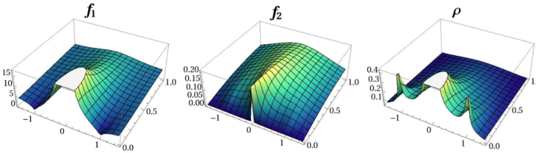
We display plots of the metric factors for random values of the parameters in Figure 2.
4.2 Calculation of the boundary entropy
We use (2.13) to obtain a simple expression for the holographic entanglement entropy,
| (4.8) |
The integral is logarithmically divergent at and we have to introduce a cutoff , as illustrated in Figure 3. Note that the integration converges at the -cap points . The holographic entanglement entropy can be found with the help of the following regularized integrals,
| (4.9) |
where is a large cutoff, is a UV cutoff, and . We obtain the following expression,
| (4.10) |

As discussed in [25, 16] the cutoff in the bulk has to be related to the UV in the CFT as follows. After a change of variables , the asymptotic region is mapped into and the metric (2.9) behaves as,
| (4.11) |
The boundary of the CFT is located at and the region for which we calculate the entanglement entropy is the interval . As explained in Appendix B, mapping the -slicing coordinates to Poincaré slicing coordinates allows to relate the cutoff to the CFT cutoff as follows,
| (4.12) |
This relation introduces the dependence of the entanglement entropy on the length of the interval as well as dependence on the parameter .
| (4.13) |
To isolate the boundary entropy, we consider the difference of the entanglement entropy for arbitrary value of and a reference value , while keeping (i.e. the cosmological constant and hence the central charge), (i.e. the length of the interval) and the UV cutoff fixed.
| (4.14) |
Note that parameterizes the un-attracted scalars moduli in the asymptotic region with charges .
4.3 BCFT interpretation
The result for the holographic boundary entropy should be compared to a boundary entropy of the dual CFT. While a complete analysis will not be performed here, following [25, 16], the result (4.14) can be compared with a weak coupling expression for the boundary entropy of a BCFT with compact bosons of radius obeying Dirichlet boundary conditions [26],
| (4.15) |
Note that in a supersymmetric setting, the number of compact bosons is related to the central charge, and in our case we have,
| (4.16) |
Comparing the holographic result (4.14) and the CFT result (4.15) the central charge dependence match and we can identify radius dependence in (4.15) with the dependence on the value of the un-attracted scalar moduli . For the case of the D1/D5 the relevant CFT is the orbifold and in [25, 16] a precise identification of the boson radius in (4.15) and the asymptotic value of the dilation which takes the role of in (4.14) was made. Hence, the holographic boundary entropy (4.14) is a U-dual generalization of this result.
5 Explicit solutions for one and caps
In this section, we shall adapt the method of parametrization by auxiliary poles, constructed in [2] for regular solutions, to the case of generalized solutions. We shall work out explicitly the solutions with a single region and an arbitrary number of -caps.
5.1 Auxiliary pole parametrization of regular solutions
We begin by reviewing the solution, given in [2], of the constraints (2.4) in terms of auxiliary poles, and a parametrization of the functions in terms of light-cone variables ,
| (5.1) | |||||
where , and . Since the functions are meromorphic, the functions must also be meromorphic. Moreover, the harmonic function associated with must obey Dirichlet vanishing conditions,
| (5.2) |
The meromorphic functions may be parametrized by a finite number of simple poles,
| (5.3) |
The poles , the residues , and the asymptotic parameters must be real. The above parametrization will apply to the regularity conditions of Section 2.3 for regular solutions, as well as to the regularity conditions of Section 3.2 for generalized solutions.
For regular solutions, avoiding curvature singularities requires and to have common zeros. Therefore, we take to have the form,
| (5.4) |
In turn, to avoid an extra auxiliary pole or an extra zero at infinity, we need the number of auxiliary poles to be related to the number of physical poles, . Finally, regularity of the at the auxiliary poles, and constancy of the sign of , requires the relation,
| (5.5) |
With this parameterization, and this choice of sign, all regularity conditions of Section 2.3 for regular solutions will be satisfied.
5.2 Solutions with -caps
Before we adapt the light-cone auxiliary pole parametrization to the case of solutions with a single asymptotic region and -caps, we shall present here the general covariant form of and for such solutions. With only a single region, we have one double pole in both and , which we place at . We shall look for solutions which in addition have -caps, which correspond to no poles at all in , and to simple poles in ,
| (5.6) |
As a result, we have
| (5.7) |
The -cap configuration requires to be real. Reality of for real requires to be real as well. Charge conservation requires
| (5.8) |
The constraint and inside must now be enforced on these data. It is not known how to do this explicitly in the covariant formulation, but an explicit solution in terms of a light-cone parametrization does exist, and will be given in the next subsection.
5.3 Auxiliary pole parametrization of solutions with -caps
We begin by listing the data of the solution: we have poles of at and with . Only one of these poles of is double, while the other poles are simple. Therefore, we must have auxiliary poles. For the solutions with -caps, the functions must have poles, at . This makes sense, because in the regular solutions, was allowed to have poles only at the zeros of in the upper half-plane. But the complex zeros of our have all moved to the real axis, and so the poles of have also moved to the real axis, specifically to the points .
In the light-cone parametrization, one begins by considering the combination,
| (5.9) |
The poles of on the real axis at , may be realized in two different ways, namely,
- 1.
has a simple zero for ; or
- 2.
is finite and non-zero at ; this behavior arises when and have equal residues at so that , with have simple poles at .
In general, a -duality transformation will map one behavior into the other. Hence, without any loss of generality, we can construct a solution in which has simple zeros at . Since tends to a constant as we will have,
| (5.10) |
where is a real constant, and we have introduced the following notation,
| (5.11) |
Since the degrees of and coincide, will indeed tend to a finite constant at . The points are the remaining auxiliary poles. Using , the parametrization of (5.1), we solve for the remaining light-cone functions. The zeros of generically become poles of , but the auxiliary poles of should not appear as zeros in . Thus, we set,
| (5.12) |
Since we must have for real , the residues and must be real. Since should be regular at the points , we make the familiar requirement (5.5). The expression for is readily obtained from , and we find,
| (5.13) |
It is straightforward to check that the inequality is satisfied in the interior of , using identically the same arguments as were used in [2] for regular solutions. This completes the explicit construction of solutions for the case with a single with -caps.
5.4 Calculation of the data of the covariant form
The independent data, and their counting, of our construction are as follows,
| (5.14) | |||||
giving a total of , of which two are artifacts. Remarkably, this result is the one expected from the counting of the physical parameters of the solutions, i.e. charges obeying charge conservation and null-charge conditions (a total of conditions), plus the values of un-attracted scalars in the region.
The entanglement entropy will involve the charges and the positions . The are readily extracted from the data, and we find,
| (5.15) |
for . The components can be readily obtained using equation (5.1). The expressions for and are provided by (5.12), all other data being primary. Note that the contribution of cancels out. Finally, is given in terms of by charge conservation.
5.5 Calculation of the entanglement entropy
Recall our key result for the entanglement entropy,
| (5.16) |
To evaluate this integral, we make use of the covariant form (5.6), as well as of the integrals (4.9). The holographic entanglement entropy then becomes,
| (5.17) |
Note that the last term contributing to the entanglement entropy in (5.17) is a finite contribution which depends on the position of the auxiliary poles, i.e. on the moduli (such as the null charges) of the -caps. Subtracting the UV divergent part in (5.17) associated with the bulk contribution and using the relation (4.12), one obtains the boundary entropy of a BCFT associated with the caps. This formula seems to suggest that the -caps are providing boundary conditions which define a BCFT for the bulk CFT which is fixed by the charges and value of scalar moduli of the asymptotic region. These configurations generalize the solution with two -caps, discussed in Section 4 and depicted in Figure 1.
6 probe-branes and the funnel solution
In this section we shall construct a simple solution which has only one asymptotic region and features one -funnel.
6.1 The -funnel solution with one asymptotic
A single asymptotic region requires a single pole in on the real axis, which we place at . An extra pole in the bulk of may then be chosen to be at the point by further use of the symmetry. The vanishing of on the real axis requires, however, having a mirror pole at as well. We are thus led to the following Ansatz,
| (6.1) |
with real and positive. The associated vector of meromorphic functions is given by,
| (6.2) |
Regularity as requires overall charge conservation,
| (6.3) |
Reality of on the real axis requires and to be real, as well as . Combining both requirements, we use the following parametrization,
| (6.4) |
where is real. The first constraint of (2.4) imposes the following conditions,
| (6.5) |
which implies . The second constraint of (2.4) imposes the conditions . Similarly to the solution presented in Section 4.1, both sets of conditions may be solved within the restricted sector, with the help of two real parameters and ,
| (6.6) |
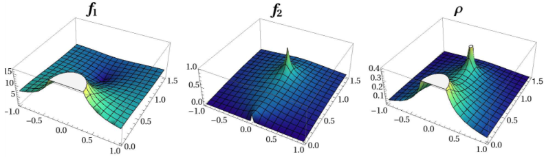
The vector will be real, as required by our construction, provided . The metric factors are given by,
| (6.7) |
Interestingly, as far as the metric factors are concerned, the solution has the same form as the one given for the -caps given in Section 4.1, with the poles at replaced by poles at . We display plots of -funnel metric factors in Figure 4.
6.2 Calculation of the entanglement entropy
We use (2.13) to obtain a simple expression for the holographic entanglement entropy,
| (6.8) |
where we have introduced the familiar cutoff for the asymptotic region. The entanglement entropy for the -funnel clearly also diverges at the support of the funnel, namely . We shall use an independent regulator (see Figure 3 (c)). The dependence on both regulators is straightforward to compute, and we find,
| (6.9) |
Comparing the entanglement entropy (6.9) with (4.10), one recognizes important similarities and differences between the solution with an -funnel and two -caps. The first term in (6.9) is the same UV divergent term, as the one in (4.10) and is associated with the asymptotic region. The second term in (6.9) presents a new divergence which is associated with the -funnel. It can be traced back to the fact that the location of the -funnel at is an infinite geodesic distance away from points in .
Note that the holographic boundary away from poles of is simply given by the boundary of the factor, which is a -dimensional space. Consequently, it seems that the -funnel produces a UV divergent contribution to the entanglement entropy from degrees of freedom which are localized on the -dimensional boundary of the space where the CFT lives. It would be interesting to understand the holography and the interpretation of the entanglement entropy for solutions with -funnels better, but we shall leave this investigation for future work.
7 Discussion
In this paper we have relaxed the regularity conditions on the half-BPS string junction solutions found in [2]. This allows for more general configurations which contain -caps and -funnels.
The -cap introduces a curvature singularity localized on the boundary of , it carries a three-form charge which is null. We provided evidence that this solution corresponds to a fully back-reacted solution of a -brane (at its -duality orbit) with world-volume.
The -funnel has no curvature, or any other, singularities, but it introduces a new asymptotic region emanating from the bulk of with asymptotic geometry. We provided evidence that the -funnel corresponds to the fully back-reacted solution of a -brane (and its -duality orbit) with world volume, which carries electric field on . The -funnel does not arise as a limiting case of the regular half-BPS string-junction solutions of [2], in contrast to the -cap. The -funnel may be obtained as a limit, however, from solutions where has at least two connected boundary components, such as those constructed in [4].
The simplest -cap and -funnel solutions are constructed letting the meromorphic functions have two extra first-order poles on the boundary or in the bulk of respectively. In principle, we could consider, for both solutions, the limit in which the two poles approach each other, leading to a second order pole on the boundary. Expanding the relevant functions close to this pole and introducing polar coordinates, we find that blows up as . Remarkably, the solution shares some of the features of the -cap and -funnel. Using the expressions (2.5) we see that both the and metric factors vanish at the pole, as expected for a -cap solution. However, the second-order pole is now at an infinite geodesic distance, as expected for the -funnel.
The reader might ask whether these generalization are special compared to other singular solutions which might be constructed by general relaxation of the regularity conditions. The answer to this question is twofold. First, the -cap and the -funnel are sufficient to account for all BPS probe-branes in listed in table 1. Second, the -cap and the -funnel can be produced by taking degenerating limits of regular half-BPS junctions solutions, and can therefore be viewed as constituting components of the boundaries of the moduli space of regular solutions. We illustrate these degeneration limits in Figure 5. As was already discussed in [4], for a Riemann surface with more than one boundary component, the limit where one boundary degenerates to a point produces a new asymptotic region which we can now interpret as a funnel.

Since the positions of the poles of on the disk are moduli of the regular half-BPS solution one can consider degenerations where poles come together in groups. For appropriately chosen charges this will lead to a dividing degeneration with -caps. A more complete analysis of the boundary of moduli space of regular half-BPS junctions is under investigation [27].
Completely regular solutions with only one asymptotic region are precluded by charge conservation. Thus, the simplest regular solutions are of the Janus type, and are dual to interface CFTs. We made explicit use of the fact that the charge vector of -caps is null to construct solutions with only one asymptotic region. Each such solution is dual to a BCFT, and we have presented solutions with an arbitrary number of -caps, and discussed in detail the simplest case with . Our construction turns out to be similar in spirit to the one presented for BCFTs in four dimensions in [28, 29] which, in turn, were based on the construction of half-BPS junction solutions in [30, 31]. In [28, 29], the role of the -caps is played by singularities associated with five-branes. In [28], the singular half-BPS solutions were matched precisely with the field theoretic classification of BCFTs [32]. It would be interesting to explore the BCFT dual to our solutions with -caps.
Finally, we also used the -funnel to construct solutions with only one asymptotic region. At present, the interpretation of these solutions remains, however, less clear. While the holographic entanglement entropy for the BCFT, constructed using -caps, gives an UV divergent part related to bulk of the CFT and a finite boundary entropy, the boundary entropy for the solution with the -funnel has an additional divergence coming from the funnel. One possible interpretation is that the degrees of freedom residing in the funnel make an extensive contribution to the entanglement entropy, which is related to the additional UV-divergent term. In the dual CFT, a contribution this kind could not arise from a finite number of degrees of freedom localized on the interface. It would be very interesting to investigate properties of the solutions containing funnels further.
Acknowledgements
We thank Tadashi Takayanagi for very helpful comments on a first draft of this paper. The work of Eric D’Hoker, Michael Gutperle was supported in part by NSF grant PHY-07-57702. The work of Marco Chiodaroli was supported in part by NSF grant PHY-08-55356.
Appendix A Uplift of -cap solutions to ten dimensions
To clarify the interpretation of the solutions with -cap singularities, in this appendix we will consider their uplift to ten dimensions. In general, these solutions will be characterized by a pole of located on the boundary. We will fix the pole at throughout this section without any loss of generality. Then, close to the singularity we have the expansion
| (A.1) |
with real and . We can always find a gauge transformation rotating and so that the only non-zero components are and . In this case, the leading behavior of the solution at the singularity will be the same as a solution which we know how to interpret in ten dimensions [22].
The translation of the old solutions in our language is given by the relations [2],
| (A.2) |
Using these relations, we can then express the ten dimensional fields of [22] in the auxiliary poles parameterization of our solutions. In particular, we will need the ten-dimensional dilaton and K3 metric factor,
| (A.3) |
As explained in Section 5.3, a simple pole of on the boundary corresponds to two possible behaviors of the functions : either has a simple zero while the functions () are non-zero, or is non-zero, but the functions have first order poles. In general there exists a -duality transformation mapping the two different behaviors into each other. Without any loss of generality we will study the second kind of behavior expanding the relevant functions as follows,
| (A.4) |
with . There are two possibilities. If , after some algebra we get,
| (A.5) |
In this case we need for the solution to satisfy the inequality . The radial behavior is exactly the one expected from a fundamental -brane. Similarly, in case we obtain the expressions,
| (A.6) | |||||
| (A.7) |
with . This -dependence is the one expected for a fundamental -brane. All other -cap singularities, e.g. the one corresponding to fundamental strings and -branes, can be generated acting with a -duality transformation on the solutions above.
Appendix B Relating the AdS and CFT UV-regulators
In this appendix we discuss the relation of the UV cutoff in the bulk AdS and the UV cutoff on the CFT side. The discussion follows [25, 16] and is included here to make the present paper self-contained.
Near a pole of the metric becomes asymptotically , since the three sphere is not important for the relation of the cutoffs we will only consider the three dimensional part of the metric which takes the following form for and finite.
| (B.8) |
One can absorb the constant by a shift in ,
| (B.9) |
and one gets
| (B.10) |
In this limit we can perform an coordinate change which maps the slicing to a Poincare slicing by
| (B.11) |
The terms as of the metric becomes
| (B.12) |
The half-space on which the BCFT lives has . Note that near the boundary the change of coordinates is more complicated. In particular, the coordinate change (B.11) is not smooth at . For the purposes of calculating the holographic entanglement entropy we consider a point and never approach . However, for other calculations, such as the boundary OPE, the limit has to be considered and the discussion is much more involved.
The metric (B.12) in the limit takes the standard form of in Poincaré coordinates and standard rules of AdS/CFT apply in identifying a cutoff for the coordinate and the UV cutoff of the CFT. It follows from (B.11) and (B.9) that the UV cutoff of the CFT and the cutoff in the -slicing coordinate are related by
| (B.13) |
Appendix C Calculating entanglement entropy for an -funnel
The holographic entanglement entropy for the funnel is given by,
| (C.14) |
where we have introduced the familiar UV cutoff for the asymptotic region. The entanglement entropy for the -funnel clearly also diverges at the points of support of the funnel, namely . This is an IR divergence, for which we use an independent regularization . To evaluate the integrals, we set , so that,
| (C.15) |
We split up this integral as follows,
| (C.16) |
where
| (C.17) |
Evaluating these integrals gives,
| (C.18) |
is the integral encountered in the calculation for the -cap,
| (C.19) |
Putting all together, we find,
| (C.20) |
which gives the following expression for the funnel entropy,
| (C.21) |
References
- [2] M. Chiodaroli, E. D’Hoker, Y. Guo, M. Gutperle, “Exact half-BPS string-junction solutions in six-dimensional supergravity,” [arXiv:1107.1722 [hep-th]].
- [3] D. Bak, M. Gutperle and S. Hirano, “A Dilatonic deformation of AdS(5) and its field theory dual,” JHEP 0305 (2003) 072 [hep-th/0304129].
- [4] M. Chiodaroli, E. D’Hoker, M. Gutperle, “Open Worldsheets for Holographic Interfaces,” JHEP 1003, 060 (2010). [arXiv:0912.4679 [hep-th]].
- [5] J. M. Maldacena, “The large N limit of superconformal field theories and supergravity,” Adv. Theor. Math. Phys. 2 (1998) 231 [Int. J. Theor. Phys. 38 (1999) 1113] [arXiv:hep-th/9711200].
- [6] A. Van Proeyen, “Superconformal Algebras,” IN *VANCOUVER 1986, PROCEEDINGS, SUPER FIELD THEORIES* 547-555.
- [7] E. D’Hoker, J. Estes, M. Gutperle, D. Krym and P. Sorba, “Half-BPS supergravity solutions and superalgebras,” JHEP 0812 (2008) 047 [arXiv:0810.1484 [hep-th]].
- [8] J. D. Brown and M. Henneaux, “Central Charges in the Canonical Realization of Asymptotic Symmetries: An Example from Three-Dimensional Gravity,” Commun. Math. Phys. 104 (1986) 207.
- [9] J. Raeymaekers, K. P. Yogendran, “Supersymmetric D-branes in the D1-D5 background,” JHEP 0612 (2006) 022. [hep-th/0607150].
- [10] C. Bachas and M. Petropoulos, “Anti-de-Sitter D-branes,” JHEP 0102 (2001) 025 [arXiv:hep-th/0012234].
- [11] J. Raeymaekers, “Open String Attractors,” JHEP 0704 (2007) 075 [arXiv:hep-th/0702142].
- [12] T. Takayanagi, “Holographic Dual of BCFT,” [arXiv:1105.5165 [hep-th]].
- [13] M. Fujita, T. Takayanagi, E. Tonni, “Aspects of AdS/BCFT,” [arXiv:1108.5152 [hep-th]].
- [14] A. Karch, L. Randall, “Open and closed string interpretation of SUSY CFT’s on branes with boundaries,” JHEP 0106 (2001) 063. [hep-th/0105132].
- [15] L. J. Romans, “Selfduality For Interacting Fields: Covariant Field Equations For Six-Dimensional Chiral Supergravities,” Nucl. Phys. B 276 (1986) 71.
- [16] M. Chiodaroli, M. Gutperle and L. Y. Hung, “Boundary entropy of supersymmetric Janus solutions,” JHEP 1009, 082 (2010) [arXiv:1005.4433 [hep-th]].
- [17] S. Ryu and T. Takayanagi, “Holographic derivation of entanglement entropy from AdS/CFT,” Phys. Rev. Lett. 96 (2006) 181602 [arXiv:hep-th/0603001].
- [18] M. Chiodaroli, M. Gutperle, L. -Y. Hung, D. Krym, “String Junctions and Holographic Interfaces,” Phys. Rev. D83, 026003 (2011). [arXiv:1010.2758 [hep-th]].
- [19] R. Dijkgraaf, “Instanton strings and hyperKahler geometry,” Nucl. Phys. B 543 (1999) 545 [arXiv:hep-th/9810210].
- [20] N. Seiberg, E. Witten, “The D1 / D5 system and singular CFT,” JHEP 9904 (1999) 017. [hep-th/9903224].
- [21] C. Bachas, J. de Boer, R. Dijkgraaf and H. Ooguri, “Permeable conformal walls and holography,” JHEP 0206, 027 (2002) [arXiv:hep-th/0111210].
- [22] M. Chiodaroli, M. Gutperle and D. Krym, “Half-BPS Solutions locally asymptotic to and interface conformal field theories,” JHEP 1002 (2010) 066 [arXiv:0910.0466 [hep-th]].
- [23] K. Dasgupta and S. Mukhi, “BPS nature of 3-string junctions,” Phys. Lett. B 423 (1998) 261 [arXiv:hep-th/9711094].
- [24] A. Sen, “String network,” JHEP 9803 (1998) 005 [arXiv:hep-th/9711130].
- [25] T. Azeyanagi, A. Karch, T. Takayanagi, E. G. Thompson, “Holographic calculation of boundary entropy,” JHEP 0803 (2008) 054-054. [arXiv:0712.1850 [hep-th]].
- [26] S. Elitzur, E. Rabinovici and G. Sarkissian, “On least action D-branes,” Nucl. Phys. B 541, 246 (1999) [arXiv:hep-th/9807161].
- [27] M. Chiodaroli, E. D’Hoker, and M. Gutperle, in preparation.
- [28] B. Assel, C. Bachas, J. Estes and J. Gomis, “Holographic Duals of D=3 N=4 Superconformal Field Theories,” JHEP 1108 (2011) 087 [arXiv:1106.4253 [hep-th]].
- [29] O. Aharony, L. Berdichevsky, M. Berkooz and I. Shamir, “Near-horizon solutions for D3-branes ending on 5-branes,” arXiv:1106.1870 [hep-th].
- [30] E. D’Hoker, J. Estes and M. Gutperle, “Exact half-BPS Type IIB interface solutions I: Local solution and supersymmetric Janus,” JHEP 0706 (2007) 021 [arXiv:0705.0022 [hep-th]].
- [31] E. D’Hoker, J. Estes and M. Gutperle, “Exact half-BPS Type IIB interface solutions II: Flux solutions and multi-Janus,” JHEP 0706 (2007) 022 [arXiv:0705.0024 [hep-th]].
- [32] D. Gaiotto, E. Witten, “S-Duality of Boundary Conditions In N=4 Super Yang-Mills Theory,” [arXiv:0807.3720 [hep-th]].