The Augmented Fast Marching Method for Level Set ReinitializationThanks: This work was supported by the University at Buffalo, State University of New York.

A two-dimensional computational domain with a uniform grid spacing of $h$ has an embedded interface, $\Gamma$. The goal is to calculate the signed distance function to the interface without any spurious motion of $\Gamma$. To accomplish this the Eikonal equation with $F=1$,

is solved in the entire computational domain. In the fast marching method upwind derivatives are used to approximate $\nabla\phi$. This enforces a causality on the propagation of information. Consider two points, $\boldsymbol{x}$ and $\boldsymbol{y}$, where the point $\boldsymbol{x}$ is closer to the interface than point $\boldsymbol{y}$. Due to the fact that $F=1$ and the use of upwind derivatives the value at any given point only depends on those points closer to the interface. Thus the value $\phi(\boldsymbol{y})$ may depend on the value of $\phi(\boldsymbol{x})$, but the value of $\phi(\boldsymbol{x})$ will never depend on the value of $\phi(\boldsymbol{y})$. This leads to an ordering of the nodes which needs to be maintained throughout the reinitialization procedure.

When using the fast marching method three sets of nodes are maintained. The first are accepted nodes, $A$, which are those nodes where a value of $\phi$ has already been calculated and accepted. The second set are trial nodes, $T$. The trial set contains those nodes which might next be added to the accepted set. Finally, the distant set, $D$, are those nodes which are too far from the interface to be added to the accepted set. Due to the causality of the FMM we are guaranteed that if $\boldsymbol{x}\in A$, $\boldsymbol{y}\in T$, and $\boldsymbol{z}\in D$ then $|\phi(\boldsymbol{x})|<|\phi(\boldsymbol{y})|<|\phi(\boldsymbol{z})|$. See Fig. 1 for the relationship between the three set of nodes.

To initialize the FMM mark all nodes in the domain as in the distant set. Define a grid cell $\Omega_{i,j}$ as the region enclosed by the four points $\boldsymbol{x}_{i,j}$, $\boldsymbol{x}_{i+1,j}$, $\boldsymbol{x}_{i,j+1}$, and $\boldsymbol{x}_{i+1,j+1}$. Identify all grid cells which contain the interface and mark the nodes associated with these cells as in the accepted list.

The standard fast marching method can be initialized by explicitly calculating the level set function for all nodes associated with cells containing the interface. Define a bicubic interpolation function, $P(\boldsymbol{x})$, approximating the level set function in a given cell. In the absence of gradient information the bicubic function can be obtained by ensuring that $P(\boldsymbol{x}_{m,n})=\phi_{m,n}$, $\partial_{x}P(\boldsymbol{x}_{m,n})=\partial_{x}\phi_{m,n}$, $\partial_{y}P(\boldsymbol{x}_{m,n})=\partial_{y}\phi_{m,n}$, and $\partial_{xy}P(\boldsymbol{x}_{m,n})=\partial_{xy}\phi_{m,n}$ for $m={i,i+1}$ and $n={j,j+1}$ at grid cell $\Omega_{i,j}$. All derivatives of the level set can be obtained by using standard finite difference approximations. At every grid point $\boldsymbol{x}_{i,j}$ in the initially accepted the list the point $\boldsymbol{y}$ is calculated such that $p(\boldsymbol{y})=0$ and $\nabla p(\boldsymbol{y})\times(\boldsymbol{x}_{i,j}-\boldsymbol{y})=0$. The distance to the interface is then $\|\boldsymbol{x}-\boldsymbol{y}\|_{2}$. This results in a second-order approximation to the true distance function [9].

After the initial accepted list is determined the remaining grid nodes are updated in an ordered manner. All grid nodes adjacent to the initial accepted list are given estimates of the distance function by solving an upwind discretization of Eq. (1),

where $D_{x}^{\pm}$ and $D_{y}^{\pm}$ are one-sided derivatives. The appropriate derivative is chosen based on the direction of neighboring accepted nodes. Let the node being updated be $\boldsymbol{x}_{i,j}$ with nodes $\boldsymbol{x}_{i-1,j}$ and $\boldsymbol{x}_{i,j+1}$ in the accepted list. To first order the derivatives in this case would be $D_{x}^{-}\phi=(\phi_{i,j}-\phi_{i-1,j})/h$ and $D_{y}^{+}\phi=(\phi_{i,j+1}-\phi_{i,j})/h$, where $h$ is the grid spacing. In general solving Eq. (2) will result in two real roots, $\tilde{\phi}_{1}$ and $\tilde{\phi}_{2}$ [9]. The smallest root which is larger than the surrounding stencil nodes is taken to be the accepted value. In the example case given the solution would be the smaller of $\tilde{\phi}_{1}$ and $\tilde{\phi}_{2}$ that is larger than both $\phi_{i-1,j}$ and $\phi_{i,j+1}$.

The remaining grid nodes are updated in the following fashion. The grid node in the trial list with the smallest level set value is moved into the accepted list. All nodes surrounding the newly accepted node which are in either the trial or distant lists are updated by solving Eq. (2). Any updated nodes in the distant list are moved into the trial list. This procedure is repeated until no nodes remain in the trial list. The next node to be added to the accepted list is easily obtained if the trial list is maintained as a sorted list such as a heap.

Initialization of the augmented fast marching method proceeds in a manner similar to the standard fast marching method. Let the grid cell $\Omega_{i,j}$ contain the interface. It is possible to define a bicubic interpolant over this cell using the given data. As this work was designed to work with the gradient augmented level set method it is assumed that the level set value, $\phi$, and the gradient of the level set, $\nabla\phi=\boldsymbol{\psi}=\left(\psi^{x},\psi^{y}\right)$, is available at the four grid nodes associated with $\Omega_{i,j}$. To compute the bicubic interpolant it is necessary to define $\phi_{xy}$ at the four grid points. This value is calculated as the average of the derivatives of the gradient field. At any point $\phi_{xy}=(D_{x}\psi^{y}+D_{y}\psi^{x})/2$ where $D_{x}$ and $D_{y}$ represent the centered second order finite difference approximations to the first derivative.

To initialize the augmented fast marching method all nodes associated with grid cells containing the interface are moved into the accepted list. Values for the level set, $\phi$, the gradient of the level set, $\boldsymbol{\psi}$, and the Hessian of the level set, $\boldsymbol{H}$, are calculated at each of these initially accepted points.

The initialization follows a technique developed for accurately calculating the curvature of level set functions [13]. Let the grid node $\boldsymbol{x}_{i,j}$ be in the initially accepted list. A $3\times 3$ sub-grid is centered at $\boldsymbol{x}_{i,j}$. The spacing of this sub grid is taken to be $\alpha h$, where $\alpha<1$ and $h$ the uniform grid spacing, see Fig. 2. Each of the nine points in the sub-grid have a signed distance function value calculated by minimizing the function $\|\boldsymbol{y}-\boldsymbol{x}_{0}\|^{2}_{2}$ subject to $P(\boldsymbol{y})=0$, where $P(\boldsymbol{x})$ is the bicubic interpolant over the grid cell $\Omega_{i,j}$ and $\boldsymbol{x}_{0}$ is the sub-grid point. The required derivatives are then obtained by standard second-order finite difference schemes using the sub-grid data. Due to the small sub-grid size the accuracy of the initialized values is extremely high, see the results sections for details about the convergence rate.

The remaining grid nodes are updated in an ordered manner. Nodes adjacent to the initially accepted list are updated by solving the discretization of Eqs. (3)-(5). These nodes are placed into the trial list which is kept as a heap sort to ensure the fast retrial of the node with the smallest level set value. The node in the trial list with the smallest value is placed into the accepted list and any non-accepted adjacent nodes are updated. If an adjacent node is in the distant list it is moved into the trial list. This procedure is repeated until no nodes remain in the trial list.

The updating procedure for the AFMM is more involved than the standard FMM. In the standard FMM a single nonlinear equation needs to be solved, Eq. (2). In the 2D AFMM there are six nonlinear equations. The solution obtained will depend on the particular discretization of the equations given in Sec. 3. In the case of two accepted nodes, one in each Cartesian direction, the discretization chosen is

The operator $D_{x}^{\pm}$ and $D_{y}^{\pm}$ represent the appropriate one-sided derivatives at the grid point to be updated, see Sec. 2.3 or Ref. [9] . Also note that due to symmetry there are three components to the Hessian matrix which we denote as $\phi_{xx}=H^{xx}$, $\phi_{yy}=H^{yy}$, and $\phi_{xy}=H^{xy}$. It is worth noting that this particular discretization allows for the solution of the level set and gradient field first, Eqs. (12)-(14). Once a valid solution set $\{\phi,\boldsymbol{\psi}\}$ is calculated the solution of the Hessian field, Eqs. (15)-(17) can be determined.

To determine if a calculated solution to the gradient system, Eqs. (12)-(14), is valid acceptance criteria similar to the classical FMM must be implemented. Due to the larger amount of information the acceptance criteria of the classical FMM is augmented. In addition to requiring that the solution level set value be larger than either of the grid point’s neighbors it is also required that the calculated gradient be in the same general direction as the neighboring nodes. For example, let the nodes $\boldsymbol{x}_{i+1,j}$ and $\boldsymbol{x}_{i,j+1}$ be accepted nodes when updating the value at $\boldsymbol{x}_{i,j}$. In this case the chosen finite difference approximations would be the stencils for the positive one-sided derivatives in each direction, $D_{x}^{+}$ and $D_{y}^{+}$. Let $\tilde{\phi}$ and $\tilde{\boldsymbol{\psi}}=\left(\tilde{\psi}^{x},\tilde{\psi}^{y}\right)$ be solutions to Eqs. (12)-(14). A valid solution set would satisfy $\tilde{\phi}\geq\phi_{i+1,j}$, $\tilde{\phi}\geq\phi_{i,j+1}$, $\tilde{\boldsymbol{\psi}}\cdot\boldsymbol{\psi}_{i+1,j}\geq 0$, and $\tilde{\boldsymbol{\psi}}\cdot\boldsymbol{\psi}_{i,j+1}\geq 0$. If the solution set $\{\tilde{\phi},\tilde{\boldsymbol{\psi}}\}$ satisfies these conditions then it is taken as valid.

When updating the values at $\boldsymbol{x}_{i,j}$ it is possible that only a single neighboring node is in the accepted list. In this case the discretization is modified to account for the reduced amount of information. To use only information in the $x$-direction the system becomes

The general idea is to replace derivatives in the direction not present ($y$-direction in this case) with the equivalent $x$-direction derivatives. A similar formulation can be made for using information only from the $y$-direction and is given in Appendix A.

The extension to three dimensions is straightforward. Explicitly writing Eqs. (3)-(5) results in ten equations,

The quantities of interest are the level set function $\phi$ and derivatives of $\phi$ up to second order. Using upwind finite difference approximations for the first derivative this results in a set of ten nonlinear equations for the ten unknowns.

In the three dimensional case initialization of a grid point $\boldsymbol{x}_{i,j,k}$ occurs over a $3\times 3\times 3$ sub-grid centered on $\boldsymbol{x}_{i,j,k}$. To use numerical approximations of the derivatives it is not necessary to determine the level set value for all 27 points on this sub-grid as only 19 points are used during the derivative calculations. As in the two-dimensional case these sub-grid points have their distance to the interface calculated by minimizing $\|\boldsymbol{y}-\boldsymbol{x}_{0}\|^{2}_{2}$ subject to $P(\boldsymbol{y})=0$, where $P(\boldsymbol{x})$ is the tricubic interpolant over the grid cell $\Omega_{i,j,k}$. When computing the tricubic coefficients it is sufficient to ensure that the following values are satisfied at the eight corner nodes of the grid cell: $\phi$, $\phi_{x}$, $\phi_{y}$, $\phi_{z}$, $\phi_{xy}$, $\phi_{xz}$, $\phi_{yz}$, and $\phi_{xyz}$. Assuming that only the level set and the gradient of the level set are available during reinitialization any higher order derivatives are obtained by averaging the appropriate derivatives. For example the third-order derivative necessary for the tricubic function is given by $\phi_{xyz}=(D_{yz}\psi^{x}+D_{xz}\psi^{y}+D_{xy}\psi^{z})/3$, where $D_{xy}$ is the finite difference approximation to $\partial_{xy}$.

Updating the remaining grid points proceeds in the same fashion as the two-dimensional case. Due to the higher number of dimensions there are seven possibilities from where information will be propagating. The specific discretizations for all possibilities have been presented in Appendix B.

One consequence of choosing the above discretizations is that the solution for the gradient system, Eqs. (12)-(14) for the two dimensional case, can be computed first. Once a valid solution set $\{\phi,\boldsymbol{\psi}\}$ is calculated the solution for the Hessian field, Eqs. (15)-(17) can be determined. In practice this is done by first computing for the gradient field in the entire domain. This not only results in level set and gradient functions at every grid point, it also determines the proper ordering to ensure that upwind derivatives are calculated correctly. The Hessian field is then obtained by solving Eqs. (15)-(17) using this pre-determined ordering.

The algorithm for the augmented fast marching method can be summarized thusly:

1. 1.

   Mark all nodes as in the Distant list.

2. 2.

   Initialize all nodes associated with cells containing the interface by explicitly solving for the signed distance function on a sub-grid centered at the node. Derivatives of the level set are calculated by standard finite difference approximations on this subgrid. Move these nodes into the Accepted list.

3. 3.

   For all nodes in the Distant list that lie next to a node in the Accepted list calculated updated values by solving Eqs. (6)-(8) in 2D or Eqs. (24)-(27) in 3D. Move these nodes into the Trial list.

4. 4.

   Select the node with the smallest level set value in the Trial list and move it into the Accepted list. All nodes next to the newly accepted grid point in either the Trial or Distant list have updated values calculated by solving Eqs. (6)-(8) in 2D or Eqs. (24)-(27) in 3D. Any node that is updated and in the Distant list is moved into the Trial list.

5. 5.

   Repeat Step 4 until the Trial list is empty.

6. 6.

   Calculate the Hessian field by solving Eqs. (9)-(11) in 2D or Eqs. (28)-(33) in 3D. Update nodes using the same order as they were added to the Accepted list.

The accuracy of a fast marching method depends on the order in which nodes are updated. A standard error analysis is difficult due to the nonlinear nature of the systems involved. Instead sample analytic solutions for a circular interface of radius $R_{0}$ are considered. This interface is to be reinitialized on a grid with a uniform spacing of $h$. Consider the AFMM updating of a grid point given by $\boldsymbol{x}_{i,j}=\left(x,x\right)$, $x>0$, and $\sqrt{2x^{2}}<R_{0}$. This point lies on the domain diagonal. In this situation it is known that the grid points to the right, $\boldsymbol{x}_{i+1,j}$, and above, $\boldsymbol{x}_{i,j+1}$, are closer to the interface than $\boldsymbol{x}_{i,j}$, Fig. 3. If the neighboring nodes have the exact solution prescribed the error of node $\boldsymbol{x}_{i,j}$ can be investigated.

Consider the gradient system, Eqs. (6)-(8). Using the exact solution for nodes $\boldsymbol{x}_{i+1,j}$ and $\boldsymbol{x}_{i,j+1}$ the level set, $\phi$, and gradient vector, $\nabla\phi=\boldsymbol{\psi}=\left(\psi^{x},\psi^{y}\right)$, at $\boldsymbol{x}_{i,j}$ can be calculated as

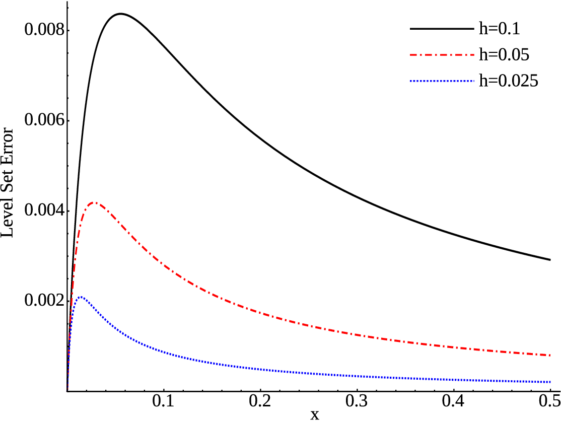
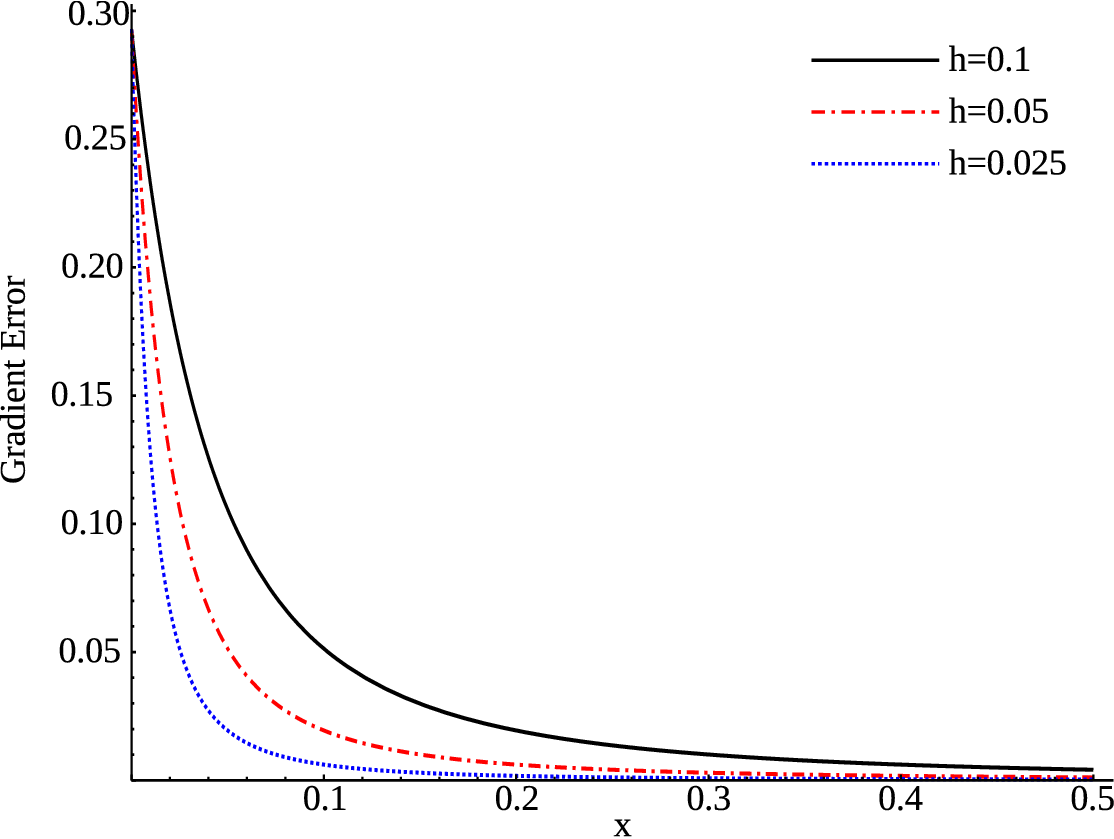
The true solutions are $\phi_{true}=\sqrt{2x^{2}}-R_{0}$ and $\psi_{true}^{x}=\psi_{true}^{y}=1/\sqrt{2}$. The error of the level set is calculated as $\phi-\sqrt{2x^{2}}+R_{0}$ while the error of the gradient vector is $\sqrt{\left(\psi^{x}-1/\sqrt{2}\right)^{2}+\left(\psi^{y}-1/\sqrt{2}\right)^{2}}$, where $\phi$, $\psi^{x}$, and $\psi^{y}$ are given in Eqs. (34) and (35). These errors are shown in Fig. 4 for locations ranging from $x=0$ to $x=0.5$ and grid spacings of $h=0.1,0.05,\textrm{and }0.025$.

From the results shown in Fig. 4 it becomes apparent that as the grid size decreases the overall error decreases for both the level set and gradient vector. The maximum error of the level set function observes a first-order convergence. The gradient vector, on the other hand, has a fixed error of $\left(\sqrt{2}-1\right)/\sqrt{2}$ as $x$ approaches zero irregardless of the grid spacing. This result should not be unexpected. As $x$ approaches the origin the variation of the gradient field increases inversely to the distance from the origin. For example, given a circular interface and a point $\boldsymbol{x}=(x,x)$ the exact variation of the x component of the gradient field in the x-direction is given by $\partial_{x}\psi^{x}=1/\left(2\sqrt{2}x\right)$. As the distance from the origin decreases due to a smaller grid spacing the variation in the gradient field will increase by an inverse amount. This results in a fixed error being introduced into the system near the origin. Despite this $\mathcal{O}(1)$ error of the gradient field the overall error decreases rapidly. As the Hessian system depends on the solution of the gradient vector it should be expected that the errors for the Hessian field, and thus the curvature, will increase as one approaches the origin.

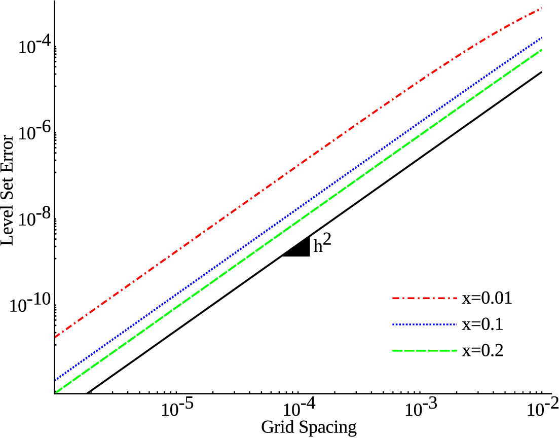
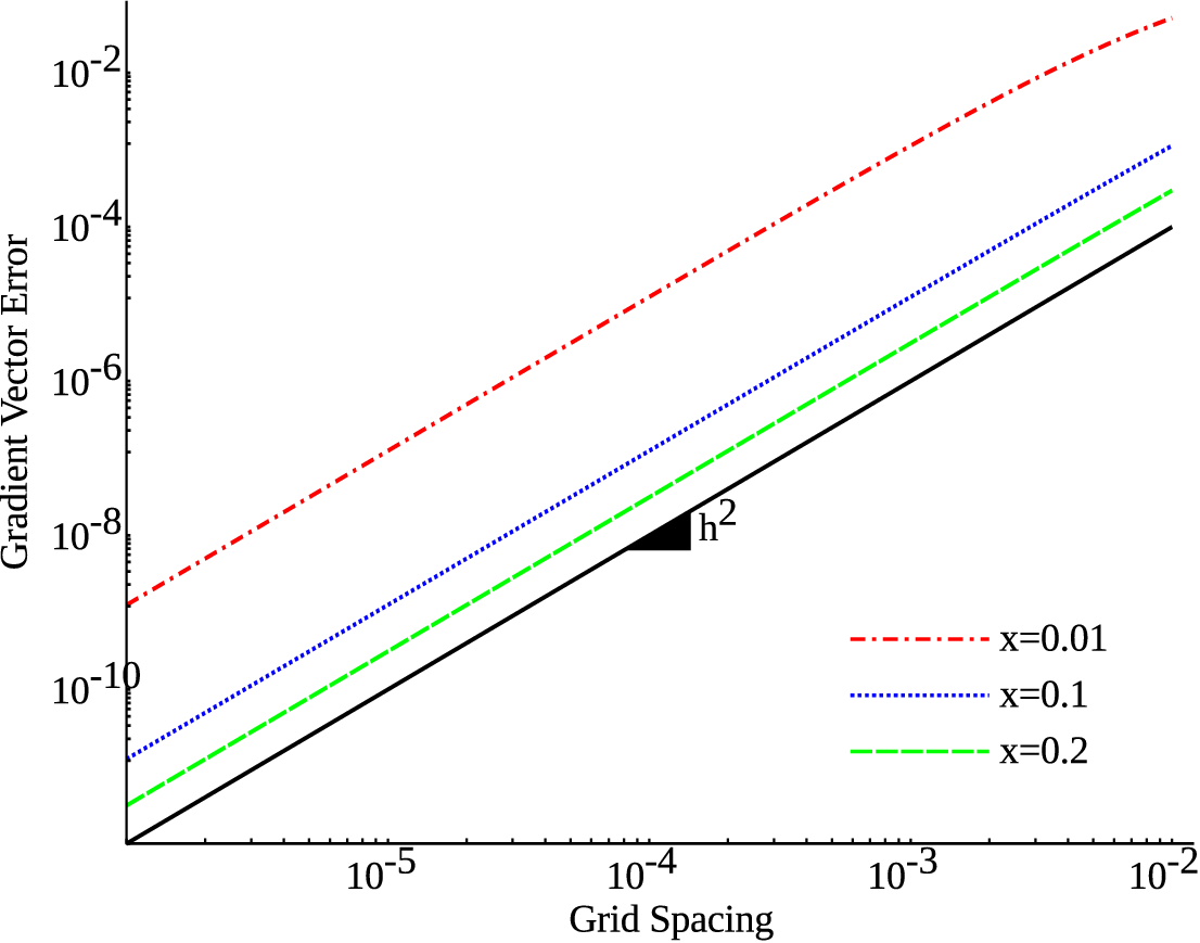
To conclude this section it should be noted that the error at any given point will decrease for both the level set and gradient vector. As an example the error for the level set and gradient vector are shown in Fig. 5 for the points $x=0.01,0.1,\textrm{and }0.2$ using grid spacing ranging from $10^{-6}$ to $10^{-2}$. For the three points considered second-order convergence is observed for both the level set and gradient vector solutions.

The accuracy of the initialization scheme presented in Sec 3.1 is shown here. A circle of radius 1 with an initial level set given by $\phi_{0}=e^{x^{2}+y^{2}}-e$ is considered. The resulting convergence rate is seen in Fig. 6

It is observed that the convergence rate for the level set is approximately $4^{th}$-order, for the gradient field it is $3^{rd}$ order, for $\phi_{xx}$ and $\phi_{yy}$ $2^{nd}$-order convergence is seen, and the $\phi_{xy}$ value is $1^{st}$-order accurate.

First consider a unit circle with the initial level set of $\phi_{0}=e^{x^{2}+y^{2}}-e$. Sample level set and curvature results at grid sizes ranging from $20^{2}$ to $500^{2}$ are shown in Figs. 7 and 8. The level set contours shown utilize the additional information provided by knowledge of the derivatives of the level set function. Even in the coarsest mesh, $20^{2}$, the level set is extremely smooth and the curvature field is smooth outside of the interface. At such a coarse mesh there are not enough grid points to accuractly describe the large variations of curvature which occurs in the region given by $\phi<0$. As the number of grid points increases this error vanishes.

Considering the results shown in Sec. 4.1 errors will be reported for both the entire domain and for the local region around the interface given by $|\phi|\leq 9h$. This width was chosen based on the stencils needed for a $5^{th}$-order WENO local level set scheme [18]. To account for the fact that the curvature grows as $1/\sqrt{x^{2}+y^{2}}$ as one approaches the center of the given level set function all curvature errors are reported as $(\kappa-\kappa_{e})/\kappa_{e}$ where $\kappa$ is the curvature using the AFMM and $\kappa_{e}$ is the exact curvature. The errors for the unit circle are given in Figs. 9 and 10.

Despite the use of first-order finite difference approximations the resulting level set is second-order accurate and the gradient is $\mathcal{O}(h^{3/2})$ in the entire domain while the curvature is $\mathcal{O}(h)$. When only considering the region close to the interface this increases to $\mathcal{O}(h^{5/2})$ for both the level set and gradient fields and $\mathcal{O}(h^{3/2})$ for the curvature field.

The convergence results verify the conclusion obtained in Sec. 4.1. The large variation in the gradient vector as one approaches the center of the circle creates a uniform error that can not be overcome. The fact that the $L_{2}$-norm does converge indicates that this error is localized around the origin. This is further supported by the convergence of both the $L_{2}$ and $L_{\infty}$-norms in the region given by $|\phi|\leq 9h$.

Next consider an elliptical interface with a major axis of 1.5 and a minor axis of 0.5: $\phi_{0}=(x/1.5)^{2}+(y/0.5)^{2}-1$. Results for various grid sizes are presented in Figs. 11 and 12. As for the unit circle the level set field is smooth even at coarse meshes. As the grid becomes finer the level set field becomes smoother, particularly along the long axis of the ellipse. The curvature field is also smooth, even for the extremely coarse grid. For all of the grids the curvature field has the same qualitative shape. An issue with the curvature can be observed towards the center of the ellipse. This is due to the gradient vector field having a sharp discontinuity in that region. This is illustrated in Fig. 13, which shows the right half of the reinitialized solution on a $50^{2}$ grid. The resulting gradient vector field switches sign when crossing the x-axis, resulting in errors being introduced into the Hessian, and therefore the curvature, solution.

As in the unit circle case the convergence of the elliptical interface is presented for both the entire domain and the region given by $|\phi|\leq 9h$. The exact solution was calculated by explicitly determining the signed distance function on a $4000^{2}$ grid. The convergence results for the elliptical case match those of the unit circle.

This section concludes by presenting three additional sample interface. In each case a coarse grid of $50^{2}$ is compared to a fine grid of $500^{2}$. Results are for two circles of radius 0.75 centered at $(0.8125,0.4125)$ and $(-0.8125,-0.4125)$, a Cassini oval with an initial level set of $\phi_{0}=\left((x-a)^{2}+y^{2}\right)+\left((x+a)^{2}+y^{2}\right)-b^{4}$ with $a=0.99$ and $b=1.01$, and a star interface given by $\phi_{0}=\sqrt{x^{2}+y^{2}}-1+\sin(5\theta)/4$ with $\theta=\textrm{ArcTan}(y/x)$, see Figs. 16 to 18.

In all three cases level set and curvature fields at the coarse grid qualitatively match those at the finer grid. Errors in the curvature field are again demonstrated in regions where level set fronts collide, such as the diagonal in the two circle case of Fig. 16, the y-axis of the Cassini oval, Fig. 17, and along several of the diagonals of the star shape, Fig. 18. These error diminish as the grid is refined.