Free energy of alternating two-component polymer brushes on cylindrical templates
Abstract
We use computer simulations to investigate the stability of a two-component polymer brush de-mixing on a curved template into phases of different morphological properties. It has been previously shown via molecular dynamics simulations that immiscible chains having different length and anchored to a cylindrical template will phase separate into stripes of different widths oriented perpendicularly to the cylindrical axis. We calculate free energy differences for a variety of stripe widths, and extract simple relationships between the sizes of the two polymers, and , and the free energy dependence on the stripe width. We explain these relationships using simple physical arguments based upon previous theoretical work on the free energy of polymer brushes.
Introduction
Polymer brushes are highly tunable systems that have recently attracted considerable attention in the scientific community. This is mainly due to the already large number of technological applications in which they are used, but also to the promising role these materials hold for the future. Apart from their well known role in the stabilization of colloidal particles [1], polymer brushes are also used as lubricants, in chromatographic devices and in adhesives, and their use has recently been proposed in a variety of biotechnological applications including drug delivery and drug-biocompatibility enhancers [2, 3, 4, 5]. Generally speaking, they offer an ideal platform that provides control over the physical and chemical properties of solid and fluid surfaces.
Polymer brushes are basically dense systems of polymer chains having one end tethered to a non-adsorbing surface, and they have been thoroughly studied theoretically and numerically on different geometries (see [6, 7, 8, 9, 10, 11, 12, 13, 14, 15] and references therein). The equilibrium properties of these systems typically depend on the molecular weight of the chains, their grafting density, and the quality of the solvent. Although we have a good qualitative understanding of homogeneous and single components brushes, for which scaling arguments have been successfully put forward, the problem becomes very complex as soon as we deal with non-homogeneous systems with multi-component or nonlinear chains.[16, 17]
Of particular relevance for the present paper is the work done by Stellacci and collaborators [18, 19, 20, 21, 22] where basically a two-component brush of immiscible ligands having different length has been shown to phase separate into striped phases of different widths when anchored to spherical and cylindrical templates. What is surprising is not the phase separation in itself, but rather the formation of the striped phase and its not well understood dependence on the mismatch in polymer length. Microphase separation is also expected in more traditional mismatched two-component polymer-brushes [23], where potential applications in stimuli-responsive systems and nanotemplating have recently attracted great attention to the field (see ref [24] and references therein). Being able to control pattern formation at the nanoscale is a core element in the production of novel materials via the process of self-assembly.
Direct coarse grained molecular dynamics simulations by Glotzer et al. have clearly indicated the driving forces behind the formation of these phases as the difference between the chains molecular weight, and the overall height of the brush itself [19, 21, 22, 25, 26]. Very recently, a coarse-grained model for two-component polymer mixtures of different length has also been put forward, and the formation of different phases as a function of length mismatch on a planar geometry has been analyzed, revealing the presence of striped phases in these systems as well [23].
Unlike other numerical work that focused on the details of the de-mixing transition, in this paper we focus exclusively on the origin of the microphase separation. We use numerical simulations to compute free energies of an inhomogeneous two-component polymer brush to understand how molecular weight and overall brush height affect the stability and width of the striped phases. Specifically, we focus on the case of a cylindrical solid template where stripes have been shown to form promptly both numerically and experimentally [26, 22], and we compute, at constant grafting density and template radius, how the system free energy changes when imposing stripes of different width and height on the template. Our results indicate that what limits macrophase separation into a two-phase region, thus leading to the stabilization of the striped phase, is the elastic strain that builds up in the polymer brush formed by the mismatched (exposed) polymer segments.
Methods
To ensure that our data are not affected by the lateral tension due to the immiscibility of the two polymer types, and that we are indeed measuring exclusively the free energy difference arising from the chains’ length mismatch and overall brush morphology, we simulate systems in which the only difference between the two polymer types is their length. This is equivalent to setting the line tension between the stripe’s boundaries that comes directly from the immiscibility term in the pair potential between the two polymer types equal to zero. As a consequence, we are required to lock in place the position of the anchoring monomers to prevent the different chains from trivially mixing.
Polymers are modeled as sequences of spherical beads of radius linearly connected via a harmonic potential , with . Any two monomers in the system interact via the soft and purely repulsive dissapative particle dynamics (DPD) simulation potential:
where and indicate the identity of the polymer and refers to the identity of the monomer. Here is the length of a polymer of type . All the results that follow use . Each polymer is grafted to a fixed point on the outer surface of a cylindrical template of radius via the same harmonic potential tethering the consecutive monomers in a chain. In all our simulations we considered a total number of polymers arranged in a homogenous grid having square symmetry. The polymer identity is finally selected to generate alternating stripes of width . For a lateral grafting density of the polymers equal to , our system contains one-polymer-wide rings, making the possible values of , when equal number of polymer types are considered . Figure 1 shows snapshots of typical initial configurations for and . This particular geometry is selected because we find that test unconstrained simulations of immiscible chains always lead to stripe formation perpendicular to the cylindrical axis. This result has also been observed in [26].


Given the size of the system we carried out our simulations using the molecular dynamics package LAMMPS [27] with Langevin dynamics in the ensemble. Dimensionless units are used throughout this paper. The timestep size was set to ( is the dimensionless time).
Our goal is to compute the free energy difference between systems having different stripe width , while keeping everything else unaltered, as a function of the difference between the lengths and . To compute the system free energies we use the thermodynamic integration method [28]. The idea is to introduce a fictitious potential
which acts between any two monomers in the system. For the chains are ideal and the system free energy is independent of the specific grouping of the polymer types; as we recover the system of interest. The free energy of the full system can then be extracted by performing the following integral
| (1) |
In practice, we perform simulations for several values of , and numerically compute the integral above.
Results
To get insight into the problem we first consider the case in which ; that is, only one chain type is present in the system. Figure 2a shows our numerical data for the free energy cost associated with the partitioning of the two polymer species into alternate stripes of different on a cylinder of radius and lateral grafting density , as a function of and for polymer lengths and . This specific lateral grafting density was selected because unconstrained simulations under this condition lead to prompt microphase separation for moderate values of polymer immiscibility. Furthermore, a sufficiently large value of lateral grafting density guarantees large enough differences in free energies as a function length mismatch.


Our data show that the most favorable state corresponds to that having the largest number of stripes (i.e. the smallest value of ). The inset on the same figure shows how the free energy difference grows with the length of the chain . These results can be qualitatively understood by referring back to the theory of polymer brushes on flat surfaces and its extension to spherical and cylindrical surfaces [9, 29]. The key point is that the main contribution to the free energy cost per chain associated with a polymer brush has an inverse dependence on the the lateral chain-to-chain grafting distance .
| (2) |
where is the height of a brush made with polymers of length grafted on a planar surface. Although in our system the location of the grafting lattice on the cylindrical surface is independent of and therefore the total grafting density of the system is kept constant at all times, different distributions of the chains on the lattice result in different local densities. Crucially, when considering the free energy contribution due to the different lateral organization of the chains, one can consider our system with as a polymer brush with twice the lateral grafting distance of that relative to . Clearly the latter system cannot be straightforwardly described with Eq. 2 due to the free boundaries of the brush, nevertheless we expect that for the role of the boundary should become negligible. If we now introduce the dimensionless parameter defined as
| (3) |
the argument above leads to clear upper-bounds on the value of . Specifically, we expect in the flat limit, and for , independently of chain length. Our numerical results are indeed within these bounds.
Figure 2b shows plotted as a function of for different values of . has a nontrivial dependence on ; nevertheless, simple geometrical arguments can be used to understand at least qualitatively the overall behavior of these curves. Figure 3 shows a sketch of the expected chain distributions for and for the simpler case of a flat surface. For small values of the problem is dominated by boundary effects, and we can imagine the chains equally sharing the overall space per stripe available to them.


It is immediately obvious that the free energy difference between and per chain should be very small indeed. In both cases the chains can be accommodated into space as a sequence of blobs of diameter equal to twice the grafting distance . A similar argument can be made for . The main extra cost in free energy per polymer for a growing should come from the weak entropic stretching of the polymers next to the grafting surface and should weakly grow as .
When becomes large, the free energy of the system is dominated by chains in the bulk of the stripe. In this regime the blob size of the outer chains is larger than that of the inner chains. Assuming a generic size profile for the blobs of the form where and is fixed by the constraint , one can estimate the free energy per stripe as . Given that there are particles in each stripe, the free energy per particle on a flat interface reads as
| (4) |
It is difficult to extract from our simulations, but from visual inspection of the brush profiles one should expect , leading to functional forms for having the typical saturating behavior shown in our data.
In the current form the data do not collapse onto a universal master curve. In fact, the free energy difference of shorter chains tends to grow faster than that of the longer ones. This result is quite revealing as it directly reflects on the nontrivial interactions between neighboring regions of grafted polymers.
Such interactions will cease as soon as the mutual distance between two neighboring regions is larger than twice the side spread of the polymers at the boundaries. Clearly this will happen sooner for the short polymer than for the longer ones. We should be able to account for this difference by rescaling of with . We find the best collapse for . This result suggests a length-scale, , controlling the extent of the side interactions that scales as . Figure 4 shows the data collapse into a universal master curve .

Let’s now turn our attention to the case in which . It would be desirable to develop a simple way of extending our results to the more general case. In particular, we are interested in understanding whether it is possible to map a system having different polymer lengths to a system of a single polymer type of length (and .)
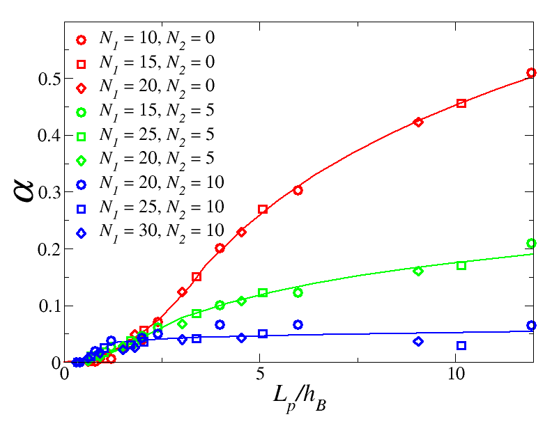
Figure 5 shows as a function of for different values of at and . The results for are also shown as a reference. As the cause for the free energy gap between the different configurations rests in the difference , to properly compare the data coming from systems having different values of , when computing we subtracted from the measured free energies the constant core free energy of the underlying full brush of height , . When , we define as .
It is comforting to report that indeed it is possible to systematically collapse all of the data corresponding to different values of at a given (fixed) into unique curves; however, we cannot collapse data coming from different values of . This result clearly points to the fact that the universal curve previously described for also has a nontrivial dependence on : . In principle, this shouldn’t come as a surprise for brushes grafted on a curved surface, in fact, the effect of the “interior” layer of monomers is to increase the effective radius of the cylinder to which the reduced system would be grafted onto, and to decrease the grafting density of the effective brush of length ; both are variables the free energy depends on (see Eq. 2).
Simple geometrical arguments can be used to estimate the change in lateral grafting distance. Following [29], we can write the change in lateral grafting spacing as we radially move away from the cylinder surface of an amount as . For short polymers and at the relatively high densities of our systems we have . It follows that . Simultaneously, the effective polymer of length would be grafted onto a cylinder of radius . The ratios appearing in the brush free energy should then be adjusted to introducing a predictable dependence on in the problem. Although this argument suggests an overall increase in free energy for the system at a given , it isn’t obvious how it will affect the dimensionless ratio . Clearly this correction should factor out in the large limit or for .
Our numerical data show that is quite sensitive to . Specifically, tends to flatten as increases. This is most likely explained by the fact that the base of the effective chain of length is not really grafted in place, but the layer of polymers below allow for significant reorganization of the base due, for instance, to their compressibility. Because of the blob-size dependence on the distance from the surface, on a convex template the chains become systematically more laterally compressible as is increased. The net result is a flattening of the free energy difference as a function of . Unfortunately, we find that our data for different values of cannot be collapsed by a simply rescaling of the free energy with a power of , indicating a subtle interplay between and the height of the bottom layer.
Conclusions
In summary, we analyzed the relative stability of the striped phases arising from the de-mixing of immiscible polymers on a cylindrical template as a function of the width of the stripe, the length mismatch between the chains, and the overall length of the brush. We set numerical bounds for the free energy gap between an alternating (many thin stripes) and a fully de-mixed (two wide stripes) phase, and found that indeed the former becomes more and more favorable as the mismatch between the chains’ lengths, is increased. We also found that when appropriately normalized the free energies as a function of stripe width for different values of can be collapsed into unique master curves that only depend on the overall length of the lower brush . Finally we discussed the possibility of reducing a two-component system of chains having lengths into a simpler single component system of chains of length . Our results are fully consistent with previous molecular dynamics simulations on this problem in identifying the key parameters setting the width of the stripes in the polymer length mismatch , and the overall length of the shorter brush together with the degree of chain immiscibility.
In all our data the direct line tension coming from the pair potential between chains of different types has been set to zero. This term would add to the free energy balance a predictable contribution of the type , where is the height of the polymer brush formed by the lower chains and is the number of phase boundaries. Clearly has a minimum for and is large for small . The balance between the line tension and the configurational free energy computed in this paper should therefore set the width of the stripe. More work in this direction is currently underway.
ACKNOWLEDGMENTS
This work was supported by the American Chemical Society under PRF grant No. 50221-DNI6.
References
- [1] D. H. Napper, Polymeric Stabilization of Colloidal Dispersions (Academic Press, London, 1983).
- [2] E. S. Dragan, ed., New trends in ionic (Co)polymers and hybrids (Nova Science, New York, 2007).
- [3] R. C. Advincula, W. J. Brittain, and K. C. Caster, eds., Polymer Brushes (Wiley-VCH, Weinheim, 2004).
- [4] P. Somasundaran, ed., Polymer Brushes: Applications in Biotechnology (Taylor & Francis, 2006).
- [5] M. A. C. Stuart et al., Nature Materials 9, 101 (2010).
- [6] S. T. Milner, Science 251, 905 (1991).
- [7] P. G. de Gennes, Scaling Concepts in Polymer Physics (Cornell University Press, Ithaca, NY, 1979).
- [8] K. Binder, ed., Monte Carlo and Molecular Dynamics Simulations in Polymer Science (Oxford University Press, 1995).
- [9] D. Daoud and J. P. Cotton, J. Phys. (Paris) 43, 531 (1982).
- [10] S. Alexander, J. Phys. (Paris) 38, 983 (1987).
- [11] A. Halperin, M. Tirrell, and T. P. Lodge, Adv. Polym. Sci. 100, 31 (1992).
- [12] S. T. Milner, T. A. Witten, and M. E. Cates, Macromolecules 21, 2610 (1988).
- [13] C. M. Wijmans and E. B. Zhulina, Macromolecules 26, 7214 (1993).
- [14] C. Biver, R. Hariharan, J. Mays, and W. B. Russel, Macromolecules 30, 1787 (1997).
- [15] D. Dimitrov, A. Milchev, and K. Binder, Macromol. Symp. 252, 47 (2007).
- [16] A. G. Koutsioubas and A. G. Vanakaras, Langmuir 24, 13717 (2008).
- [17] M. Patra and P. Linse, Nano Lett. 6, 133 (2006).
- [18] A. M. Jackson, J. W. Myerson, and F. Stellacci, Nature Materials 3, 330 (2004).
- [19] C. Singh et al., Physical Review Letters 99, 226106 (2007).
- [20] J. J. Kuna et al., Nature Materials 8, 837 (2009).
- [21] R. P. Carney et al., J. Am. Chem. Soc. 139, 798 (2008).
- [22] C. Singh, A. M. Jackson, F. Stellacci, and S. C. Glotzer, J. Am. Chem. Soc. 131, 16377 (2009).
- [23] R. C. Van Lehn and A. Alexander-Katz, J. Chem. Phys. 135, 141106 (2011).
- [24] N. Ayres , Poly. Chem. 1, 769 (2010).
- [25] A. Santos, C. Singh, and S. C. Glotzer, Physical Review E 81, 011113 (2010).
- [26] C. Singh et al., Nanoscale 3, 3244 (2011).
- [27] S. J. Plimpton, J. Comp. Phys. 117, 1 (1995).
- [28] D. Frenkel and B. Smit, Understanding Molecular Simulation: From Algorithms to Applications (Academic Press, San Diego, 2002), 2nd ed.
- [29] C. Hiergeist and R. Lipowsky, J. Phys. II (France) 6, 1465 (1996).