Ensemble renormalization group for disordered systems
Abstract
We propose and study a Renormalization Group transformation that can be used also for models with strong quenched disorder, like spin glasses. The method is based on a mapping between disorder distributions, chosen such as to keep some physical properties (e.g. the ratio of correlations averaged over the ensemble) invariant under the transformation. We validate this Ensemble Renormalization Group (ERG) by applying it to the hierarchical model (both the diluted ferromagnetic version and the spin glass version), finding results in agreement with Monte Carlo simulations.
I Introduction
The renormalization group (RG) is a fundamental tool in theoretical physics [1]. It allows to characterize phase transitions and critical phenomena, by computing critical exponents and universality classes. The real space RG can be viewed as a decimation procedure that takes a system made of dynamical variables and reduces it to a smaller system, in a way which preserves, or scales appropriately, some important physical observables. Such a decimation induces a RG transformation on the system couplings, and the study of such a transformation allows one to identify critical points and critical exponents.
Real space RG transformations have been studied in great detail for homogeneous models [1], but much less is known for disordered models, that contain quenched randomness in the Hamiltonian (either random fields and/or random couplings). This is specially true for strongly frustrated models, like spin glasses (SG), for which a satisfying RG transformation is still lacking. For example, for the Edwards-Anderson SG model [2] on a -dimensional lattice all the attempts to develop a field theory by performing an -expansion around the upper critical dimension have proved to be very complicated [3, 4]. These studies have led to the discovery of fixed points different from the mean-field (MF) ones, however the implications of that are not completely clear. In particular the existence of replica symmetry breaking (RSB) fixed points in the non-mean field region has been shown only very recently [5] and estimates of critical exponents in are still not reliable.
In this framework the development of a (semi-)analytical real space RG for disordered models would be very welcome. The outcome of such a RG transformation could be well compared with Monte Carlo (MC) simulations, that provide accurate estimates of critical temperatures and critical exponents for disordered models (at a much higher computational cost).
Since the first developments of RG transformations for models with quenched disorder it was clear that one has to deal with distributions of couplings [6, 7]. But the RG transformation for an entire coupling distribution is highly non-trivial. Previous attempts of developing a real space RG for disordered systems [8] focused on transformations mapping a single sample of size to a smaller system (without loss of generality we can set the size of the smaller system to ). In formulae, we can write the mapping as the one solving a set of equations like
| (1) |
where angular brackets are thermal averages with respect to the Gibbs-Boltzmann distribution, primed quantities refer to the smaller system and the number of observables is enough to determine the new couplings . Given an ensemble of systems of size , the above transformation can be applied to each of them in order to obtain an ensemble of systems of size .
However we believe that such a mapping is suboptimal for models with quenched disorder and a better RG transformation should consider explicitly the average over the quenched disorder (as was done e.g. in Ref. [9]). What we are proposing is a mapping between probability distributions of couplings such that the following equations hold
| (2) |
The overbar represents the average over the quenched disorder (i.e. the couplings in the present case). The rationale beyond this choice is that in models with strong disorder (like SG) sample-to-sample fluctuations may dominate thermal ones.
It is worth noticing that standard RG transformations working on coupling distributions typically use Eq. (1). For example, the simplest RG transformation for the bond percolation problem in 2 dimensions () or even the more complicated one of Ref. [7] can be viewed as single sample transformations, where is the bond density by which the larger samples are generated and is the bond density of the renormalized samples (one-by-one). Instead, the new approach in Eq. (2) would prescribe to compute some physical quantity (e.g. a correlation or a probability of being connected) in the ensemble of larger systems with bond density , and to repeat the same computation in the ensemble of smaller systems with several bond densities in order to find the best value such that the physical observables match in the two ensembles. The new approach we are proposing resembles in some way the finite size scaling analysis which is performed on Monte Carlo data measured in systems of different sizes. Obviously, for models where the RG transformation is exact (like e.g. the diamond hierarchical lattices [10]) the old and the new approaches provide the same answer.
Two simple examples may help elucidating even more the limits of the RG transformation working sample by sample, Eq.(1), and thus justify the use of the one in Eq.(2), that we will call Ensemble RG (ERG). In a diluted ferromagnet with long range interactions, where couplings are positive with probability and null with probability , a single step of the decimation procedure induced by Eq.(1) typically generates all non-zero couplings (i.e. ). And this is clearly not very useful if one is willing to follow the RG flow in the plane. Moreover, in frustrated models the decimated system is typically much less frustrated than the original one: the extreme case is the transformation of a 4-spins system in a 2-spins system, being the latter unfrustrated for any coupling choice! This tendency to reduce frustration makes the RG using Eq.(1) clearly unfit to describe SG fixed points.
In principle, our ERG scheme can be applied to any disordered system. We choose here to apply it to the hierarchical model (HM), which is a particular one-dimensional long range model, whose Hamiltonian for spins can be constructed iteratively in the following way [11]:
| (3) |
In practice is the sum of interactions at different levels. We have studied three versions of this model: the ferromagnet (FM), where ; the diluted ferromagnet (DFM), where a random fraction of FM couplings are set to zero; and the SG version [12], with Gaussian couplings .
There are many reasons to test a new RG transformation on the HM. First, by properly tuning the topological factor that controls how fast the couplings intensity decays with distance, the HM can emulate a -dimensional short range (SR) model: for DFM and for SG [13]. These relations are exact around the upper critical dimensions because the long range HM and the SR -dimensional model have the same field theory at leading order. In order to have a phase transition at a finite temperature, the parameter must satisfy for the DFM and for the SG. Lower bound values correspond to lower critical dimensions (and thus ), while when the energy is no longer extensive (thus ). For in DFM and in SG, the model shows mean field critical properties (like for in SR models). So, tuning a single parameter in the HM, we can move from the MF region to a non-MF one.
The second reason to choose the HM, is that if the system is decimated by a standard block-spin transformation, the new Hamiltonian does not contain any multi-spin term (at variance to what happen on finite dimensional lattices [1]). So, considering only pairwise interactions in the RG is not an approximation for the HM. Moreover the FM version can be exactly solved in a time growing only polynomially with , since the probability distribution of the magnetization satisfies
| (4) |
where and are the magnetizations of the half systems. It is worth stressing that Eq. (4) is no more valid for the SG version of the HM, which does not admit a polynomial time solution. In Ref. [14], a generalization of Eq. (4) has been proposed to describe the distribution of the overlap in the SG version of the HM; however we will not make use of this relation, due to the difficulties in its treatment.

II Ensemble renormalization group for HM
We describe now in detail how to apply the ERG to the HM. We assume couplings to remain independent during the RG, but we allow couplings to have a different probability distribution (or a different value in the FM version) at each level : in the original HM all couplings have the same probability law, but we have seen that the RG iteration produces different couplings at different levels. In the analyzed versions, each coupling distribution is parametrized by few numbers (that is the mean for FM, the variance for SG, the fraction of non-zero couplings and the mean for DFM), otherwise the search for a solution to Eq.(2) would become too difficult. We start from an ensemble of systems with levels that we want to reduce to an “equivalent” ensemble of smaller systems of levels. The whole procedure is described in Fig. 1 for a SG HM with .
- 1.
First we compute observables , in the larger systems extracted from the original coupling distribution (in the FM the overbar can be omitted).
- 2.
Then we identify the new distributions of couplings , for the ensemble of smaller systems, i.e., we determine the new parameters of the distributions, by requiring that for any .
- 3.
Finally we build a new ensemble of systems of the original size. They are constructed joining with random couplings extracted from the original distribution two smaller systems with couplings extracted from , found at step 2.
Primed quantities refer to the smaller systems. In this case the parameters to be determined are the variances of the Gaussian distributions at each level. The first two steps are the true renormalization steps, while the latter is required to obtain a final system size, that will allow us to iterate the method, until convergence. In the disordered versions, the assumption that the renormalized coupling distributions are of the same type as the original ones is an approximation. However it can be easily improved adding extra terms in the distributions. Thermal averages are computed exactly: this is easy to do in the FM, thanks to Eq. (4), while in the DFM and in the SG we do it by exhaustive enumeration, thus limiting us to a small number of levels in the disordered cases. The average over the disorder is not exact, but taken over samples. Step 2 is actually accomplished by minimizing , and we have checked that the reached minimum is always very close to zero. Since couplings distributions are different at each level, we do not see any better option than extracting the new couplings at level in step 3 from the original distribution .
The FM version of the HM, for which exact RG equations can be written, is a benchmark for our numerical implementation of the ERG. For , that corresponds to , the critical temperature is [16], and the critical exponents are , [17], leading to using the scaling relations. To compare this critical exponent with the one for a SR 3D Ising FM, it can be shown [15] that the following equation should be used with a proper – relation
| (5) |
In the present case is close to [18].
The observables that we use in the RG equations are the correlation of the magnetization at level , normalized by those at level , with :
The denominator is needed to reduce finite size effects and to ensure that a solution to the RG equations always exists (this is not true in general for other observables, like the magnetization).


Applying the previously described procedure, the flux of couplings and correlations can be followed, see Fig. 2. If , renormalized couplings stay for a while close to the critical fixed point (FP), and then go towards the high temperature (HT) FP if or the low temperature (LT) FP if . We estimate the critical temperature as the temperature dividing the flows towards the two different FP. Please note that the HT and LT fixed points are not characterized by the usual and coupling values: the reason is that in step 3 of our procedure we put new coupling of original intensity. Nonetheless couplings flows clearly differentiate HT and LT behaviors.

In order to extract critical exponents from the RG equations, we focus on the early regime, when the coupling flows leave the critical FP. From the Wilson relation an equation relating renormalized coupling after RG steps can be obtained:
where is the scaling factor in our case. Thus, the exponent can be estimated from a fit like the one in Fig. 3. The values obtained for the critical temperature and the critical exponents in are well comparable with the known ones: extrapolates to in the large limit and the measured exponent is for (although the extrapolation of to the limit is difficult due to strong finite size effects, e.g. for ). Moreover we have checked that our numerical RG recovers the right bounds on , namely for and for .
We consider now the DFM. The Hamiltonian of the model is always the one in Eq. (3), but the couplings at level are independent random variables extracted from the distribution
At the beginning and for any , while under the RG they will differentiate. The number of parameters to be determined in the ERG is , and we use the following observables, with , to fix them:

Applying the same procedure as for the pure model, we are able to draw a flow diagram in the - plane for and determine the critical line (see Fig. 4). The validity of the phase diagram found with the ERG is confirmed by a set of MC simulations (explained later in the text) whose estimates are also shown in Fig. 4. The only disappointment about this phase diagram is that we do not find an unstable FP along the critical line as expected for a SR model [19]. However this can be explained by noticing that the exponent of this model is very small, , and so the crossover from the pure behavior can be extremely long.

Finally we study the SG version. The Hamiltonian is always the one in Eq. (3), and the couplings at level are distributed with a Gaussian law of zero mean and variance (at the beginning for any ). The assumptions that the renormalized couplings are independent and normally distributed could be released by adding extra terms in the coupling distributions [9], but we leave these generalizations for future works. In the SG case the observables used to fix the variances are normalized SG correlations at different levels:
Because of the computational costs we use , so the early regime leaving the critical FP is rather short, and the stationary regime is soon reached (with respect to the FM case). This effect is also enhanced by the disorder: indeed, even exactly at criticality, the SG ensemble contains many samples which are not critical, and the couplings of these samples flow away from critical values very fast. So, it seems unavoidable that disorder increases the instability of critical FP and consequently the uncertainty on the estimates of critical exponents. Nonetheless we can distinguish two temperature regions separated by a critical temperature (see Fig. 5 for an effective dimension and ), such that above correlations and couplings decay towards zero, while below correlations and couplings variances grow, suggesting that the system is in a SG phase. In Fig. 5 we have plotted only couplings and correlations variances measured at the lowest level , but (as in the FM, see Fig. 2) the renormalized variances at the other levels are related to those at : for example, if and if (remember that parameters at the lowest level are those which are less influenced by the coupling of the original intensity at level , because they have been renormalized more times).


Also in the SG case we are able to estimate the exponent from the flux of the couplings at early times. The procedure used is the same of that in the FM case and typical fits are shown in Fig. 6 for in the mean-field region and for below the upper critical dimension. We obtain in and in . In Fig. 7 we report (with label HM ERG) the estimates of as a function of the exponent defined as : we see that in the mean-field region () results are compatible with the expected mean-field behavior ( that corresponds to ) and, more interestingly, the critical exponent has a minimum around the upper critical dimension , , as confirmed by our MC simulations (label HM MC in Fig.7) and those in Ref. [12]. This minimum was not observed in previous RG studies [8], while it is present in SR models: in Fig. 7 we report the estimates for the EA model in [21, 15, 20] following the relation introduced previously: . The same non-monotonic behavior for the exponent has been also seen in a SG model with long range (LR) power law decaying interactions () [22, 15], also shown in Fig. 7.
III Monte Carlo simulations
In order to check critical temperatures and the critical exponent for the SG version of HM in the non-mean-field region, we have run MC simulations at several values of . Couplings are extracted from a Gaussian and from a binary distributions. We have used the parallel tempering algorithm [23], running simultaneously at different temperatures. Two replicas have been simulated in parallel, to measure the overlap between them. Equilibration has been checked by the standard method of observing the convergence of the measured observables (e.g. energy and overlap moments) to their asymptotic values. We have found that the equilibration time is MC steps for the largest sizes at smaller temperatures and we have acquired data for MC steps. For the model with Gaussian couplings we have used , while for the one with couplings, that is easier to simulate, . Averages were performed over 400 samples for the larger systems up to 2000 samples for the smaller ones.
We have run also standard MC simulations (with non parallel tempering) for the DFM at several bond concentrations ().
Critical temperatures have been estimated from the crossing points of the scale-invariant observables: these crossing points should approach the critical temperature for large sizes. In particular we study the dimensionless Binder parameter [24], defined as for the DFM and for the SG. We can construct also another scale-invariant observable from the susceptibilities, and , knowing analytically its dimension . In fact the exponent is not renormalized in LR systems. Defining for the FM and for the SG, in the whole region . Thus if we divide by its dimension, the resulting or should remain finite at the critical temperature. We can apply the same argument to the fourth moment susceptibility, obtaining another scale-invariant observable for DFM and for SG.

In Fig. 8, we plot the three scale-invariant observables, , and for different sizes as a function of the temperature for a SG HM with and a Gaussian distribution of the couplings. The crosses of the curves should approach the critical temperature, that we estimate to be . Unfortunately the data do not allow us to estimate the correction to scaling exponent . Nonetheless we can say that the Binder parameter is the observable that has the largest finite size effects. The critical temperature is compatible with the one obtained from the ERG . Please consider that the estimate from ERG is obtained with a small number of levels (and in a much faster time). In Fig. 4 we report the critical temperatures of the DFM obtained by an analysis very similar to the one just described.
To measure the critical exponent we have used the more accurate data for the model with interactions, that should be in the same universality class. We use the same observables previously described to determine the critical temperature that we estimate as for . Then we look at the values of at . The dimension of this observable is and its finite size scaling form at leading order around is described by
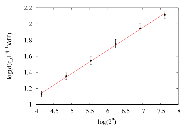
In Fig. 9 the values for at for different sizes are plotted as a function of the size of the system in a log-log scale. We have chosen this particular observable because we have seen that it has the smallest finite size effects. In this scale can be extracted via a linear fit as the angular coefficient. The straight line is the best fit that leads to . This result should be compared with the ERG estimate . They are rather different. However we know that for the estimate of exponent with the ERG method we have very large finite size effects, especially in the non mean field region (indeed we have an error of for already for the ferromagnetic case). Nevertheless the important result is that the non monotonic behaviour of with is confirmed by the MC simulations.

In Fig. 10 we have plotted the three scale-invariant observables , and for different sizes as a function of , with and . We can see that curves at different sizes collapse quite well.
IV Conclusions
Concluding, we have developed a semi-analytical real space RG method that can be used for disordered systems. The method has been applied to the hierarchical model and is able to find a SG transition also for effective dimension in the non-mean field region. The reliability of the method has been tested comparing the values of critical temperatures and critical exponents with those obtained in MC simulations. The agreement for the critical temperatures is optimal for all the version we have studied and the ERG method allows to compute them in a time much smaller than MC simulations. The critical exponents obtained with the ERG method are more affected by finite size effects than critical temperatures. In fact the error in the ERG estimate for the SG exponents is around 20%. However such a large error is not unexpected, since we find it also in the ferromagnetic case, where the correct exponent is recovered only in limit.
The ERG method is able to reproduce the correct behavior of the exponent, that shows a minimum at the upper critical value of (or ): such a behavior is predicted by the -expansion of the SG version [14] and found in our MC simulations. This accurate prediction by the ERG make us confident that the method is reliable. The present results by the ERG solve an apparent inconsistency problem between the -expansion and another real space RG approach recently proposed in Ref. [8], where the exponent was found to decrease linearly with , with no minimum at all around the upper critical dimension. In this work we have shown that such a minimum in exists if a better RG transformation is used. In particular we have shown that the right way to do renormalization when disorder is present is to consider RG on ensemble of systems and not on single samples.
This statement can be confirmed also from a comparison with the method of analysis used in MC simulations. When exponents are determined using finite size scaling (FSS), we look at the crossing point of some dimensionless quantities (like the Binder parameter) averaged over disorder for different sizes. Indeed FSS is an approximate RG where only a parameter, the temperature, is varied. In this perspective, our RG is a generalization of FSS, where we vary more parameters, and for this reason we can look at more observables. However, like in FSS, the useful observables are those averaged over the disorder.
References
- [1] D. J. Amit and V. Martin-Mayor, Field theory, the renormalization group, and critical phenomena: graphs to computers (World Scientific, 2005).
- [2] S. F. Edwards and P. W. Anderson, J. Phys. F 5, 965 (1975).
- [3] A. J. Bray and S. A. Roberts, J. Phys. C 13, 5405 (1980).
- [4] T. Temesvari, C. De Dominicis, Phys. Rev. Lett. 89, 097204 (2002). T. Temesvari, C. De Dominicis and I. R. Pimentel, Eur. Phys. J. B 25, 361-372 (2002); Phys. Rev. B 65, 224420 (2002).
- [5] G. Parisi and T. Temesvari, arxiv:1111.3313v1.
- [6] T. C. Lubensky, Phys. Rev. B 11, 3573 (1975).
- [7] A. P. Young and R. B. Stinchcombe, J. Phys. C: Solid State Phys. 8, L535 (1975).
- [8] M. Castellana, Europhys. Lett. 95, 47014 (2011).
- [9] G. Parisi, R. Petronzio, and F. Rosati, Eur. Phys. J. B 21, 605 (2001).
- [10] S. R. McKay, A. Nihat Berker, and S. Kirkpatrick, Phys. Rev. Lett. 48, 767 (1982).
- [11] F. Dyson, Commun. Math. Phys. 12, 91 (1969).
- [12] S. Franz, T. Jorg, and G. Parisi, JSTAT P02002 (2009).
- [13] We are aware that more accurate relations can be defined, as discussed exhaustively in Ref. [15]. However the scope of our comparison with short range models in the present work is only qualitative and does not pretend to be quantitative. For this reason the simplest relation is sufficient for our purpose.
- [14] M. Castellana and G. Parisi, Phys. Rev. E 82, 040105(R) (2010); Phys. Rev. E 83, 041134 (2011).
- [15] R. A. Baños, L. A. Fernandez, V. Martin-Mayor, and A. P. Young, arXiv:1207.7014 [cond-mat.dis-nn].
- [16] Y. Meurice, J. Phys. A 40, R39 (2007).
- [17] J. Godina, Y. Meurice, and M. Oktay, Phys. Rev. D 59, 096002 (1999).
- [18] A. Pelissetto and E. Vicari, Phys. Rep. 368, 549 (2002).
- [19] H. G. Ballesteros et al., Phys. Rev. B, 58, 2740 (1998).
- [20] L. Klein, J. Adler, A. Aharony, A. B. Harris, and Y. Meir, Phys. Rev. B 43, 11249 (1991).
- [21] M. Hasenbush, A. Pellissetto, and E. Vicari, Phys. Rev. B 78, 214205 (2008).
- [22] L. Leuzzi, G. Parisi, F. Ricci-Tersenghi, and J. J. Ruiz-Lorenzo, Phys. Rev. Lett. 101, 107203 (2008).
- [23] K. Hukushima and K. Nemoto, J. Phys. Soc. Jpn. 65, 1604 (1996).
- [24] K. Binder, Z. Phys. B 43 (1981) 119.