Bayesian Estimation of a Gaussian source in Middleton’s Class-A Impulsive Noise
Abstract
The paper focuses on minimum mean square error (MMSE) Bayesian estimation for a Gaussian source impaired by additive Middleton’s Class-A impulsive noise. In addition to the optimal Bayesian estimator, the paper considers also the soft-limiter and the blanker, which are two popular suboptimal estimators characterized by very low complexity. The MMSE-optimum thresholds for such suboptimal estimators are obtained by practical iterative algorithms with fast convergence. The paper derives also the optimal thresholds according to a maximum-SNR (MSNR) criterion, and establishes connections with the MMSE criterion. Furthermore, closed form analytical expressions are derived for the MSE and the SNR of all the suboptimal estimators, which perfectly match simulation results. Noteworthy, these results can be applied to characterize the receiving performance of any multicarrier system impaired by a Gaussian-mixture noise, such as asymmetric digital subscriber lines (ADSL) and power-line communications (PLC).
Index Terms:
Interference, Impulsive noise, MMSE estimation, Middleton’s Class-A noise, Gaussian-mixtures, soft-limiter, blanker, ADSL, PLC.I INTRODUCTION
Interference and noise with impulsive non-Gaussian distributions may impair the performance of several systems including communications, controls, sensors and so forth. Middleton has proposed widely accepted canonical models for interference [1, 2, 3], which are capable to characterize “intelligent” (e.g., information bearing), as well as “non-intelligent” (e.g., natural or man-made) noises. Although Middleton’s noise models were widely investigated to identify the interference behavior [1, 2, 3, 4, 5], to estimate their canonical parameters [6, 7, 8, 9, 10], and to detect finite alphabets in digital communications [11, 12, 13, 14, 15, 16], to the best of the author knowledge results for the optimum Bayesian estimator (OBE) of Gaussian sources in Class-A impulsive noise are still lacking or, at least, not widely acknowledged. Thus, the first aim of the paper is to derive the minimum mean squared error (MMSE) OBE for a scalar Gaussian source impaired by Middleton’s Class-A canonical noise. Noteworthy, such an OBE is useful also as a preprocessing stage for estimation and detection algorithms that are designed under AWGN hypotheses and, consequently, are not robust to impulsive noises [11, 17]. Although the paper derives the analytical expression of the OBE in a closed form, its use may be restricted in some practical applications due to complexity or implementation constraints. For instance, this is the case when the protection from the impulsive source has to be granted in the analogic domain either to protect the device, or to limit the input dynamic range of A/D converters. In these cases it is possible to employ simpler suboptimal devices that are robust to high noise peaks: a possibility is to resort to a blanking-nonlinearity (BN) that nulls out the received signal when it overpasses a given threshold or, alternatively, to a soft-limiter (SL) that simply clips the signal when it overpasses the threshold. In both cases, only the blanking or the clipping thresholds have to be optimized in a MMSE Bayesian sense. Actually, although the SL estimator (SLE) and the BN estimator (BNE) are suboptimal with respect to the OBE, the derivation of the optimum Bayesian thresholds is analytically much harder than the computation of the OBE expression. Anyway, the paper shows that in both cases the computation of the optimum thresholds can be formulated as the solution of a fixed-point problem [18], which is proved to always admit a solution, obtainable by standard iterative approaches with fast convergence. The comparison of the shape of the OBE curve with the simplified SLE and BNE, can intuitively illuminate whether the BNE or the SLE is the best simplified strategy. Typically, the MSE is the quantitative parameter that is used to choose among different estimators: the paper shows that the best choice among the SLE and the BNE strictly depends on the statistical characteristics of the received signal, which are summarized by the average signal-to-noise power ratio (SNR), the noise peakness, the average number of emitting noise sources, etc.. Theoretical and simulation results highlight that in almost all the scenarios (at least) one of the two suboptimal estimators does not suffer any significant MSE loss with respect to the OBE, further motivating their use.
From a practical application perspective, the OBE and the suboptimal SLE and BNE are of valuable help in those applications where the quantity of interest can be modeled, or approximated, by a Gaussian probability density function (pdf). This is the case, due to the central limit theorem (CLT) [19], when the quantity of interest is generated by the superposition of several non-dominating random quantities, as it happens for instance in multicarrier-based communication systems. In particular, asymmetric digital subscriber lines (ADSL) [20] and power-line communications (PLC) [21], which are known to face cumbersome impulsive noise scenarios [22, 23, 24, 25], can greatly benefit by employing the proposed estimators at the receiver side. More generally, the proposed estimators can be used in any multiple-input single-output (MISO) system with a high number of inputs, which is impaired by impulsive noise.
A different criterion, based on the maximization of the SNR, has been used in [17] and [26] to set the optimal SL and BN thresholds in multicarrier communication systems impaired by impulsive noise. However, while [17] and [26] consider a complex Gaussian source, this paper concentrates on real Gaussian sources (such as those involved in ADSL- and PLC-based communications. Thus, another contribution of the paper is the derivation of the maximum-SNR (MSNR) thresholds for the BN and SL of real-valued signals, which are different from those derived in [17] and [26]. Note that, while MMSE and MSNR are equivalent in pure AWGN scenarios [27] where the MMSE estimator is linear, this is not the case when the noise is a Gaussian-mixture, which leads to a non-linear MMSE estimator. Due to the fact that the MMSE and the MSNR approaches are not equivalent, they lead to SL and BN suboptimal estimators with different thresholds: this paper shows when the two thresholds are similar and, conversely, when they are different. Whether it is better to maximize the SNR or minimize the MSE depends on the specific application and design constraint. This is not the subject of the paper, which however establishes also the connection between the MMSE and the MSNR criteria: by exploiting this connection, the final contribution of the paper is the derivation of closed form expressions of the MSE and SNR for the suboptimal SL and BN estimators.
The paper is organized as follows: section II introduces the system model, while the OBE, SLE, and BNE are derived in sections III, IV, and V, respectively. Successively, section VI concentrates on the MSNR criterion, proposes a method that greatly simplifies its theoretical computation, and derives the equations to iteratively compute the MSNR-optimal thresholds for the SLE and the BLE. Section VII formally establishes the relationship between MSE and SNR, and highlights that also the theoretical MSE of the BLE and SLE can be derived with significant lower computational complexity with respect to a classical approach. Finally section VIII is dedicated to computer simulations that confirm the theoretical findings, while the conclusions are drawn in the last section.
is generally used throughout the paper for statistical expectation, while is used to make explicit that the expectation is computed with respect to the pdf of the random variable . Furthermore, is used for the derivative of with respect to .
II System Model
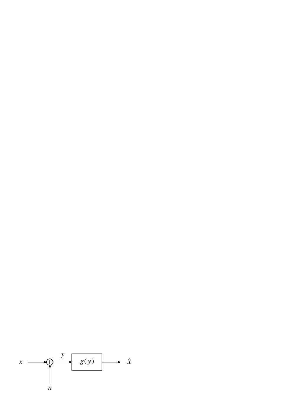
Let’s consider a zero-mean real source with average power and Gaussian pdf , impaired by a Class-A impulsive noise with average power , as shown in Fig. 1 and summarized by
| (1) |
The Class-A impulsive noise subsumes also the presence of a background zero-mean thermal AWGN , with average power . Specifically, the impulsive noise pdf is a Gaussian-mixture expressed by
| (2) |
where the weights represent the Poisson-distributed probability that noise sources simultaneously contribute to the impulsive event [2, 4]. The power associated to the simultaneous emission from noise sources is expressed by
| (3) |
where , represents the impulsive part of the noise power, is the power ratio among the AWGN and the impulsive part of the noise , and represents the average number of impulsive sources that are simultaneously active. The three canonical parameters , , and completely specify the statistical structure of the Class-A noise. In particular, low values of identify rare and highly-peaked impulsive sources, while conversely high values of makes the impulsive noise more similar to an AWGN, by a CLT argument. The interested readers are redirected to [2, 5, 4] and references therein for further details on the Class-A model, and to [6, 7, 8, 9, 10] for the estimation of the canonical parameters , , and . This paper assumes that the canonical parameters have been perfectly estimated by the observing system.
III Optimum Bayesian Estimator (OBE)
The optimum MMSE Bayesian estimator of given the observed data , is expressed by [28]
| (4) |
where represents the posterior pdf of the source for a given observation . By exploiting Bayes rules for conditional pdfs, (4) can be expressed as
| (5) |
Due to the fact that the impulsive noise is independent of , it is well known [19] that the pdf of the observed value in (1) is given by the linear convolution of the Gaussian pdf with the Middleton-A pdf in (2), as expressed by
| (6) |
where stands for the linear convolution operator and it is exploited that the convolution of two Gaussian pdfs generates a new Gaussian pdf [19] with a variance equal to the sum of the two original variances. Observing (1) it is also evident that in (5) is expressed by , which plugged in (5) leads to
| (7) |
As detailed in Appendix A, the convolution in (7) between the Gaussian pdf and can be computed in the Fourier domain by exploiting the properties of the Fourier transform (FT), leading to
| (8) |
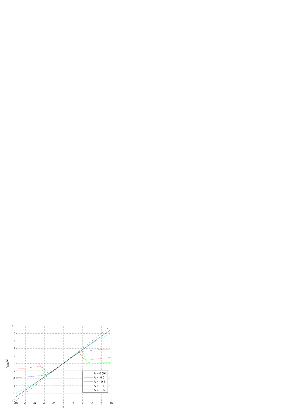
Equation (8) highlights how the OBE depends on the source average power and the noise canonical parameters , , and , through and in (3). The input-output characteristic of the OBE is plotted in Fig. 2(a) and Fig. 2(b) for several values of the parameter that controls the peakness of the impulsive noise [4]; it is evident that for very high values of , when tends to a zero-mean Gaussian pdf, the OBE tends to the well known linear-MMSE estimator, expressed by [28]
| (9) |
For lower values of , when the noise is characterizes by rare and highly peaked impulses, the optimum estimator shows a highly non-linear nature, by roughly limiting or blanking the observed values that overpass certain thresholds. The OBE expression in (8) immediately applies also to any other Gaussian-mixture noise with a finite number of mixtures, such that , and .

IV Bayesian Soft Limiter Estimator (SLE)
The OBE rather involved analytical expression (8) could prevent its use in real-time applications due to either memory or computational complexity constraints. This is especially true when the OBE analytical expression is requested to be adaptive with respect to changes of the source and of the noise statistical parameters (e.g., the average powers and , and the noise peakness factors , and . Moreover, it could be also necessary to contrast the impulsive noise in the analog domain (e.g., before A/D conversion) making OBE implementations even more challenging. For these reasons, this section investigates a simpler suboptimum estimator, namely the SLE shown in Fig. 3, which is typically employed to contrast impulsive noise [17] adding robustness to the system by clipping the signal values that exceed a given threshold . Thus, the only parameter to optimize in the Bayesian sense is the clipping threshold , which obviously would depend on the noise parameters , , and , as well as on the source power . Meaningfulness of such an optimization, which leads to the SLE, is also suggested by the OBE shapes in Fig. 2(a) and Fig. 2(b), which for certain noise parameters (e.g., resembles the SLE of Fig. 3.

The output of the SLE is expressed by a non-linear input-output characteristic : thus, the SLE estimation error depends on the selected threshold , as well as on the statistical properties of the source and the noise . This is expressed by
| (10) |
The SLE estimator is defined by selecting according to the MMSE criterion, as expressed by
| (11) |
where is the MSE cost function. Thus, in order to find it is necessary to solve
| (12) |
leading to the following integral equation
| (13) |
By substituting (2), (10) and its partial derivative in (13), Appendix B proves that is the solution of the following fixed-point equation
| (14) |
which always admits a solution. Moreover, Appendix B also proves that in (11) is locally convex for , which is equivalent to prove that locally is a contraction mapping [18]. For this reason, any numerical solution of (12) that starts from would converge to the MSE minimum, as well as the succession converges to the exact fixed point solution when goes to infinity [18]. Thus, can be numerically approximated by the following iterative algorithm
| A1: | Iterative algorithm for optimal SL threshold | |
| 1. | ||
| 2. | whi | le |
| 3. | ||
| 4. | ||
| 5. | end | |
| 6. |
In algorithm A1, represents the accuracy that is requested to the approximated solution to stop within iterations. Obviously, other iterative numerical approaches can also be used to solve (14), such as the Newton–Rapson method [18] to find the root of . Note that the local convexity of is also confirmed by the MSE plots in Section VIII: thus, it makes sense that for increasing (starting from ) the first minimum reached in (11) by the iterative algorithm is also the optimal solution, as confirmed by all the simulation results in Section VIII.
V Bayesian Blanking Nonlinearity Estimator (BNE)
Fig. 2(a) and Fig. 2(b) suggest that for highly impulsive noise behaviors (e.g., , the OBE shape resembles the BN shown in Fig. 4, where the received signal is simply blanked to zero when its absolute magnitude overpasses the threshold .

Similarly to the SLE, the goal is to derive the optimum MMSE threshold for the BN. In this case the estimation error is expressed by
| (15) |
and the MSE is expressed by
| (16) |
Thus, as detailed in Appendix C, the optimum is given by the solution of , which is equivalent to the solution of the following fixed-point equation
| (17) |
Although the fixed point problem admits a unique (non trivial) solution, as detailed in Appendix C, is a monotonically increasing function and it is not a contraction mapping [18]. Consequently, in (17) is not an attraction for the iterative algorithm A1, and an iterative algorithm that converges to the fixed point is
| A2: | Iterative algorithm for optimal BN threshold | ||
| 1. | |||
| 2. | whi | le | |
| 3. | |||
| 4. | |||
| 5. | end | ||
| 6. |
Differently from A1, in algorithm A2 the starting point has to be greater than zero (for instance to avoid the trivial solution , while controls the speed of convergence.
VI Maximum SNR (MSNR) Estimators
This section is dedicated to introduce the MSNR as an alternative criterion to optimally design the estimators. This criterion is typically employed in communication systems, such as ADSL and PLC, where the bit error rate (BER) performance depends on the SNR rather than on the MSE ([29]). In this view, [17] and [26] introduce MSNR estimators for complex Gaussian process (OFDM signals)corrupted by impulsive Gaussian mixture noise. First of all, lets observe that any estimator is in general obtained as a non-linear transformation of the observation . Anyway, the estimator output can be always decomposed as a scaled version of the input plus a distortion term , as expressed by
| (18) |
where is the linear regression coefficient that grants the distortion term is orthogonal to the input term, i.e., . However, due to the presence of the impulsive noise , the non-linearity input does not contain only the useful information . Thus, in order to define a meaningful SNR [17], it is more convenient to express the estimator output as
| (19) |
where
| (20) |
is the linear regression coefficient that grants the distortion noise is orthogonal to , as summarized by . Although in general , when the inputs are both zero-mean Gaussian and independent it holds true that [30]. Proceeding as suggested in [17], the SNR is expressed by
| (21) |
where the second equality in (21) is granted by the uncorrelation between the useful part and the distortion noise. Thus, in the MSNR sense, the optimum non-linear estimator is defined by
| (22) |
In the problem at hand, taking into account that is distributed according to (2), the computation of in the denominator of (21) and (22) can be obtained by
| (23) |
where the subscript means that the expected value is computed with respect to the Gaussian pdf associated to the Class-A Gaussian mixture. This fact suggests that the constant can be expressed as the weighted sum of other constants
| (24) |
which can be interpreted as the gain associated to the (virtual) useful components at the output of the non-linear estimator when it is separately excited by the (virtual) input . Each virtual input is the sum of two zero-mean independent Gaussian random variables and it is also zero-mean Gaussian distributed with variance . In this virtual set-up, (see Theorem 1 in [30]), it holds true that
| (25) |
where the expectation on the right-hand side of (25) involves a single-folded integral, which is much simpler to compute than the two-folded integral in its left-hand side. Moreover, last equality in (25) is attractive because it lets to exploit widely known results for the output of several non-linear devices (such as the BN and the SL) excited by Gaussian inputs [31, 32, 33, 34, 35]. Similarly, it is straightforward to derive that the average estimator output power in the numerator of (22) can be expressed as
| (26) |
where also right-hand side of (26) can exploit results widely available in the said technical literature for non-linear distortions of Gaussian random variables. However, despite the above simplifications, the solution of the functional optimization problem in (22) is not easy and the derivation of the optimum estimator in the MSNR sense is still an open problem.
Conversely, it is possible to exploit (25) and (26) if is constrained to belong to families of suboptimal estimators
| (27) |
where XX stands for either the SL or the BN, and is a scalar parameter that univocally specifies . In this case the problem reduces to a classical optimization with respect to the scalar parameter , where the optimum MSNR thresholds are expressed by
| (28) |
Thus, taking into account that the logarithm does not change the position of extreme values, the MSNR threshold is obtained by solving , which leads to
| (29) |
When the non linear device is the SL of Fig. 3, it is straightforward to derive that [31] and consequently
| (30) |
where the error function is defined as . Analogously, when the non-linear estimator is the BN of Fig. 4, by standard integration techniques it is possible to prove that
| (31) |
and, consequently,
| (32) |
Similarly, plugging and in (26), it is straightforward to derive that
| (33) |
and
| (34) |
Note that (30), (32), (33) and (34) are different from the similar equations in [17] and [26]: indeed, this paper deals with SL and BN of real random variables, while [17] and [26] consider the SL and the BN for the envelope of complex random variables. Plugging (31) and (33) in (29), after some algebraic manipulation the optimal BN threshold is the solution of the following equation
| (35) |
Analogously, plugging (30) and (34) in (29), the optimal SL threshold is the solution of the following equation
| (36) |
Equations (35) (36) can be obviously solved by root-finding numerical techniques [18], (36) However it is also possible to cast them in a fixed-point problem, which can be solved by iterative numerical approaches similar to A1 and A2. For instance the equivalent formulation of (36) is expressed by
| (37) |
It is interesting to observe that (37) can be rearranged as
| (38) |
which means that the MSNR solution for the SL is different from the MMSE solution in (14). However, when the optimal thresholds are sufficiently higher than the input standard deviation , the power of the distortion noise is quite low with , which together with (38) means that the two optimal thresholds are very close if . This specific observation for the SL can be generalized by exploiting (42), which allows to conclude that the MMSE thresholds are obtained by
| (39) |
Thus, the MMSE criterion in (39) is different from the MSNR criterion in (28) due to the absence of the square-power in the denominator of the cost function. Consequently, MMSE and MSNR approaches provide very close thresholds when : this happens for instance when the clipping threshold is sufficiently higher than , due to [see also (9)].
VII Theoretical MSE ans SNR computation
According to (10) and (15) the MSE should be computed by
| (40) |
which requests tedious double-folded integrals with respect to the signal and the noise pdfs. However, exploiting (19), the estimation error can be also expressed by
| (41) |
Thus, due to the orthogonality of and , an alternative expression for the MSE is
| (42) |
where the last equality comes from . This alternative expression is very useful for the computation of the MSE of any non-linear estimator because, differently from (40), it requests to compute only single-folded integrals, e.g., the estimator average output power by (26) and the gain by (23). Actually, for the suboptimal estimators considered in this paper, these single-folded integrals are known in closed form for any , as expressed by (33) and (31) for the BN, and (34) and (32) for the SL. Thus, plugging in these equations the values of (or ) obtained by the MMSE (or MSNR) criterion allow to compute the corresponding theoretical expressions for the MSE of the two suboptimal estimators. The same considerations hold true for the theoretical SNR, whose analytical expression in (21) requires the computation of the same single-folded integrals used for the MSE. Actually, exploiting the last equality in (21) and plugging in (42), it is derived that for any estimator the link between MSE and SNR is expressed by
| (43) |
VIII Computer Simulations
This section verifies by computer simulations the analytical results derived so far. The MSE and SNR performance of the SL and BN are computed for several sets of the Class-A canonical parameters , , and for several SNR values. All the simulated MSEs and SNRs are obtained by generating observed samples in (1). The Middleton’s Class-A noise has been generated by the toolbox [36]. The optimal MMSE thresholds for the SLE and BNE are obtained by A1 and A2, using and . The MSNR thresholds for SL and BN are obtained by Matlab numerical solutions of (36) and (35), respectively. The series with infinite terms, which are induced in all the analytical results by the Class-A pdf in (2), have been approximated by considering only the first terms (although, would be enough in most of the cases).
In Fig. 5 and Fig. 6 it is possible to observe the dependence of the optimal SL and BN thresholds on the total SNR, which is defined as . It is shown that the MMSE and MSNR (optimal) thresholds are similar for high values of (i.e., when ) and consequently the two criteria are almost equivalent. This is not the case for low (and negative) values of the , where the MMSE and MSNR thresholds tend to diverge. Moreover, it is worth noting that the MMSE and MSNR thresholds are more different for the BN rather than for the SL. This fact is more evident when , i.e., when the noise power is equally split between the AWGN and the impulsive component.
Fig. 7-Fig. 12 let better appreciate the sensitiveness of the SNR and MSE performance with respect to the SL and BN thresholds, as well as the performance penalties od the two suboptimal estimators with respect to the OBE. All the figures show that the minimum MSE and the maximum SNR are obtained for the optimal thresholds values predicted by the theory. Moreover, also the theoretical MSE and SNR derived in this paper perfectly match with the simulation results. As anticipated, in several scenarios the optimal MMSE and MSNR thresholds are almost equivalent, and consequently they provide almost the same MSE and SNR performance. However, this is not the case in highly critical scenarios where the is quite low or negative. This behavior is amplified when the AWGN noise power is not negligible with respect to the impulsive noise power (i.e., ) or when also the impulsive noise tends to be Gaussian (i.e., )). As theoretically expected, all the figures also highlight that the OBE always outperforms in MSE the SLE and the BNE. However, the SLE and BNE penalties are not dramatic, as it was expected by the fact that the OBE shapes in Fig. 2(a) highly resemble either the SLE or the BNE for several values of the canonical Class-A parameters. Interestingly, although the OBE is not the MSNR optimal estimator, in most of the cases it outperforms in SNR the MSNR-optimal BN and SL. As a final remark, the theoretical results shown in this paper can be directly employed to predict the MSE and SNR performance of multicarrier telecommunication systems (such as ADSL and PLC) that employ the proposed estimators to contrast an impulsive interference modeled as a Gaussian-mixture [25].
CONCLUSIONS
This paper has derived the MMSE Bayesian estimator for a Gaussian source impaired by impulsive Middleton’s Class-A interference. The estimator is directly extensible to any Gaussian-mixture noise. Two popular and sub-optimal estimators, namely the soft-limiter and the blanker, have been optimized both in a MSE and SNR sense, deriving also closed form expressions for their MSE and SNR. A theoretical link between MSE and SNR at the output of the estimator has been established, and scenarios when the MMSE and the maximum SNR criteria are (almost) equivalent, or different, have been clarified. The theoretical analysis and computer simulations have shown that at least one estimator, among the optimum soft-limiter or the optimum blanker, can be always used as a sub-optimum estimator with minimal performance loss with respect to the MMSE Bayesian estimator. The derivation of the optimal estimator in the maximum-SNR sense, as well as a closed-form expression for the MSE of the optimal Bayesian estimator, are still open problems for possible further research.


Appendix A OBE derivation
is used to indicate the FT of . It is also reminded that the FT of a Gaussian pdf is still a normalized Gaussian function, expressed by , where . Thus, by exploiting the convolution and derivative properties of the FT, the integral in (7) is expressed in the frequency domain by
| (44) |
By observing that , then (44) becomes
| (45) |
Thus, by the duality property of the inverse FT
| (46) |
The convolution of two zero-mean Gaussian is still a zero-mean Gaussian pdf with a variance equal to the sum of the two single variances, and consequently (46) becomes
| (47) |
Summarizing, equation (7) can be expressed by
| (48) |
which coincides with (8).
Appendix B SLE derivation
By observing (10) it is clear that is continuous with respect to and
| (49) |
Consequently, substituting (49) in (12), the optimum value is a solution of
| (50) |
which by standard integration of Gaussian density functions is equivalent to
| (51) |
where
| (52) |
and . By substituting in (51) the expression of in (2), it is recognized that the numerator
| (53) |
contains two integrals representing the convolution, and the correlation, of two zero-mean Gaussian . Due to the even symmetry of Gaussian functions, the correlation is equivalent to the convolution and the result is another zero-mean Gaussian pdf, as expressed by
| (54) |
By observing that it is possible to recognize that
| (55) |
where the convolution can be easily solved in the FT domain. Indeed, exploiting the integral property of the FT it follows that
| (56) |
which together with lets to conclude
| (57) |
To prove the existence of a solution of the fixed point equation (14), it can be observed that the relative minima and maxima of are obtained by the zeros of
| (58) |
Thus, the relative minima and maxima correspond to values that satisfy the following expression
| (59) |
Taking in mind that and , the inequality in (59) means that all the relative maxima and minima of occur when is below the angle bisector , as shown in Fig. 13. Thus, should necessarily cross the angle bisector before its first relative maximum, and consequently the fixed-point problem admits (at least) a solution. The uniqueness of the fixed-point solution (and convergence of algorithm A1 to this solution) would be granted if is a contraction mapping [18] between the fixed point solution and its first relative maximum (e.g., for , as illustrated for more clarity in Fig. 12. Actually, this is equivalent to prove that the MSE minimization problem in (11) is locally convex, i.e., for . To this end it is useful to express
| (60) |
Omitting detailed derivations, we simply observe that substituting and , the integrals in (60) can be solved exploiting (56) and (67), to obtain
| (61) |
Although it is not easy to analytically prove that for any , it can be observed that surely when in (61) is multiplied by a coefficient lower than one for any . Thus, by noting that , is always multiplied by a quantity lower than one when
| (62) |
This means that the algorithm A1 will converge toward the first minimum of the objective function in (11) every time is started with , Taking in mind that we are looking for the best soft-limiter threshold, it is reasonable to infer that the above first minimum hit by the iterative algorithm is also the optimal solution we are looking for, as also confirmed by the simulation results.
Appendix C BNE derivation
By observing (15), it is possible to proceed with the same approach of Appendix B. Due to the fact that (15) is a piecewise constant function with respect to with a discontinuity in , the Dirac’s impulse function can be exploited to handle the derivative of in this point. Thus, we obtain
| (63) |
where represents the limit from either the right () or the left (). Consequently, by direct substitution of (63)
Using for the BN the equivalent expression of (13), the optimum in the MMSE sense is obtained by equating to zero the derivative of the MSE , as expressed by
| (64) |
By exploiting the integral properties of the Dirac’s delta function, it is possible to recognize that
| (65) |
Exploiting the even symmetry of , equation (65) can be further simplified to
| (66) |
where the first integral can be split as the difference of a convolution and a correlation integral. Defining for convenience the odd function , it can be observed that the first integral (66) is expressed by
| (67) |
Using the same approach that lead to (47) in Appendix A, the integral in (67) becomes
| (68) |
Thus, observing that the second integral in (66) is just the convolution of two Gaussian zero-mean pdfs, the expression of the overall MSE derivative becomes
| (69) |
Equating to zero (69) is equivalent to find the solution of the fixed-point equation expressed by
| (70) |
which coincides with (17). The trivial solution for (70) and corresponds to a BN output equal to for any input : consequently can only be a local maximum for the MSE, with . Moreover, by observing that the zero-mean Gaussian concentrates the useful information around zero, it is intuitive that tends to decrease for values of increasing from , till reaching a minimum that can be safely assumed as the optimum threshold we are looking for. This fact is also confirmed by the shape of the MSE obtained by simulations in Figs. 5-11, which show that any classical numerical solution of will easily converge to the optimal threshold, as well as the iterative algorithm A2 that solves the fixed-point equation in (70).
More rigorously, by obvious notation equivalence, lets express in (70) as
| (71) |
Thus, the solution of the fixed point equation in (70) corresponds to . Noteworthy, as proved in the following, is a monotonic increasing function: thus the solution of , if it exists, is unique. Actually, the first derivative of is expressed by
| (72) |
where the terms for null out in the double series. Thus, due to the symmetry when the index is interchanged with , equation (72) can be rearranged as
| (73) |
By substituting in (73) the value of , , and subsumed in (70) and (71), it is readily derived that
due to the fact that all the terms inside the double series are greater than zero. Thus, it is proved that [and ] is monotonically increasing. Additionally, by observing that , it follows that
| (74) |
and consequently . Thus, as shown in Fig. 13, the BN fixed-point problem has a different structure with respect to the SL: is not a contraction mapping, which motivates the use of algorithm A2 instead of algorithm A1.
It is difficult to analytically prove that , which would guarantee the existence of the unique solution for . However, it can be observed that the MSE derivative can also be expressed as
| (75) |
Using (74), it is possible to conclude that
| (76) |
which means that the MSE plot is an increasing function when it reaches its asymptotic maximum , as intuitive and also observable in the simulation plots. Thus, a (unique) minimum should necessarily exist between the two maxima and . Otherwise, the minimization problem would have no solutions, which does not make any sense for the reasons explained before.
References
- [1] D. Middleton, “Statistical-physical models of urban radio-noise environments - part i: Foundations,” IEEE Trans. Electromagn. Compat., vol. EMC-14, no. 2, pp. 38–56 –, May 1972.
- [2] ——, “Statistical-physical models of electromagnetic interference,” IEEE Trans. Electromagn. Compat., vol. EMC-19, no. 3, pp. 106–127, Aug 1977.
- [3] ——, “Canonical and quasi-canonical probability models of class a interference,” IEEE Trans. Electromagn. Compat., vol. EMC-25, no. 2, pp. 76–106, May 1983.
- [4] L. Berry, “Understanding middleton’s canonical formula for class a noise,” IEEE Trans. Electromagn. Compat., vol. EMC-23, no. 4, pp. 337–344, Nov 1981.
- [5] D. Middleton, “Non-gaussian noise models in signal processing for telecommunications: New methods and results for class a and class b noise models,” IEEE Trans. Inf. Theory, vol. 45, no. 4, pp. 1129–1149, May 1999.
- [6] ——, “Procedures for determining the parameters of the first-order canonical models of class a and class b electromagnetic interference [10],” IEEE Trans. Electromagn. Compat., vol. EMC-21, no. 3, pp. 190–208, Aug 1979.
- [7] S. Zabin and H. Poor, “Parameter estimation for middleton class a interference processes,” IEEE Trans. Commun., vol. 37, no. 10, pp. 1042–1051, 1989.
- [8] ——, “Efficient estimation of class a noise parameters via the em algorithm,” IEEE Trans. Inf. Theory, vol. 37, no. 1, pp. 60–72, 1991.
- [9] K. Blackard, T. Rappaport, and C. Bostian, “Measurements and models of radio frequency impulsive noise for indoor wireless communications,” IEEE J. Sel. Areas Commun., vol. 11, no. 7, pp. 991–1001, 1993.
- [10] Y.-Z. Jiang, X. lin Hu, X. Kai, and Z. Qi, “Bayesian estimation of class a noise parameters with hidden channel states,” in Proc. IEEE Int. Symp. on Power Line Comm. and its Appl.(ISPLC’07), march 2007, pp. 2 –4.
- [11] S. Rappaport and L. Kurz, “An optimal nonlinear detector for digital data transmission through non-gaussian channels,” IEEE Trans. Commun., vol. 14, no. 3, pp. 266–274, Jun 1966.
- [12] A. Spaulding and D. Middleton, “Optimum reception in an impulsive interference environment–part i: Coherent detection,” IEEE Trans. Commun., vol. 25, no. 9, pp. 910–923, Sep 1977.
- [13] A. Spaulding, “Locally optimum and suboptimum detector performance in a non-gaussian interference environment,” IEEE Trans. Commun., vol. 33, no. 6, pp. 509–517, Jun 1985.
- [14] D. Middleton, “Threshold detection in correlated non-gaussian noise fields,” IEEE Trans. Inf. Theory, vol. 41, no. 4, pp. 976–1000, Jul 1995.
- [15] D. Stein, “Detection of random signals in gaussian mixture noise,” IEEE Trans. Inf. Theory, vol. 41, no. 6, pp. 1788–1801, 1995.
- [16] A. Maras, “Adaptive nonparametric locally optimum bayes detection in additive non-gaussian noise,” IEEE Trans. Inf. Theory, vol. 49, no. 1, pp. 204–220, Jan 2003.
- [17] S. Zhidkov, “Performance analysis and optimization of ofdm receiver with blanking nonlinearity in impulsive noise environment,” IEEE Trans. Veh. Technol., vol. 55, no. 1, pp. 234–242, Jan 2006.
- [18] E. Süli and D. Mayers, An introduction to numerical analysis. Cambridge Univ Pr, 2003.
- [19] A. Papoulis, Probability, Random Variables, and Stochastic Processes. McGraw-Hill, 1991.
- [20] P. Kyees, R. McConnell, and K. Sistanizadeh, “Adsl: a new twisted-pair access to the information highway,” IEEE Commun. Mag., vol. 33, no. 4, pp. 52–60, Apr 1995.
- [21] N. Pavlidou, A. Han Vinck, J. Yazdani, and B. Honary, “Power line communications: state of the art and future trends,” Communications Magazine, IEEE, vol. 41, no. 4, pp. 34–40, 2003.
- [22] W. Henkel, T. Kessler, and H. Chung, “Coded 64-cap adsl in an impulse-noise environment-modeling of impulse noise and first simulation results,” IEEE J. Sel. Areas Commun., vol. 13, no. 9, pp. 1611–1621, 1995.
- [23] M. Zimmermann and K. Dostert, “Analysis and modeling of impulsive noise in broad-band powerline communications,” Electromagnetic Compatibility, IEEE Transactions on, vol. 44, no. 1, pp. 249–258, 2002.
- [24] Y. Ma, P. So, and E. Gunawan, “Performance analysis of ofdm systems for broadband power line communications under impulsive noise and multipath effects,” Power Delivery, IEEE Transactions on, vol. 20, no. 2, pp. 674–682, 2005.
- [25] M. Nassar, K. Gulati, Y. Mortazavi, and B. Evans, “Statistical modeling of asynchronous impulsive noise in powerline communication networks,” in Proc. IEEE Int. Global Commun. Conf., December 2011, pp. 1–6.
- [26] S. Zhidkov, “Analysis and comparison of several simple impulsive noise mitigation schemes for ofdm receivers,” IEEE Trans. Commun., vol. 56, no. 1, pp. 5–9, Jan 2008.
- [27] D. Guo, S. Shamai (Shitz), and S. Verdù, “Mutual information and minimum mean-square error in gaussian channels,” IEEE Trans. Inf. Theory, vol. 51, no. 4, pp. 1261–1283, Apr 2005.
- [28] S. M. Kay, Fundamentals of Statistical Signal Processing. Vol. 1, Estimation Theory. Prentice-Hall, 1993.
- [29] J. Proakis, Digital communications. McGraw-hill, 1987.
- [30] P. Banelli, “Another useful theorem for non-linear transformations of gaussian random variables,” arXiv:1111.5950v1 (cs.IT), no. submitted to IEEE Trans. on Inf. Theory, pp. 1–7, November 2011. [Online]. Available: http://arxiv.org/abs/1111.5950
- [31] H. E. Rowe, “Memoryless nonlinearities with gaussian inputs: Elementary results,” Bell Syst. Tech. J., vol. 61, no. 7, pp. 1519–1525, Sep 1982.
- [32] J. J. Bussgang, “Crosscorrelation functions of amplitude-distorted gaussian signals,” M.I.T. RLE Technical Report, no. 216, pp. 1 –14, march 1952. [Online]. Available: http://hdl.handle.net/1721.1/4847
- [33] R. Baum, “The correlation function of smoothly limited guassian noise,” IRE Trans. Inf. Theory, vol. IT-3, pp. 193–197, Sep 1957.
- [34] W. B. Davenport Jr. and W. L. Root, An Introduction to the Theory of Random Signals and Noise. Mc Graw Hill, 1958.
- [35] P. Banelli and S. Cacopardi, “Theoretical analysis and performance of ofdm signals in nonlinear awgn channels,” IEEE Trans. Commun., vol. 48, no. 3, pp. 430–441, Mar 2000.
- [36] K. Gulati, M. Nassar, A. Chopra, N. Ben Okafor, M. DeYoung, N. Aghasadeghi, A. Sujeeth, and B. L. Evans, Interference Modeling and Mitigation Toolbox 1.6, for Matlab, ESP Laboratory, ECE Dept., Univ. of Texas at Austin, Oct 2011.
| Paolo Banelli Paolo Banelli received the Laurea degree in electronics engineering and the Ph.D. degree in telecommunications from the University of Perugia, Italy, in 1993 and 1998, respectively. In 2005, he was appointed Associate Professor at the Department of Electronic and Information Engineering (DIEI), University of Perugia, where he has been an Assistant Professor since 1998. In 2001, he joined as a visiting researcher the SpinComm group, lead by Prof. G.B. Giannakis, at the Electrical and Computer Engineering Department, University of Minnesota, Minneapolis. His research interests mainly focused on signal processing for wireless communications, with emphasis on multicarrier transmissions, and more recently on signal processing for biomedical applications, with emphasis on electrocardiography and medical ultrasounds. He has been serving as a reviewer for several technical journals, and as technical program committee member of leading international conferences on signal processing and telecommunications. In 2009, he was a General Co-Chair of the IEEE International Symposium on Signal Processing Advances for Wireless Communications. In December 2010 he has been elected as a member of the SPCOM Technical Committee of the IEEE Signal Processing Society, where he serves since January 2011. He is a co-founder (2010) and scientific co-director of ICT4Life (http://www.ict4life.it), a spin-off company of University of Perugia. |