跳到论文正文
W Papers独立论文阅读器 arXiv:1111.6714 论文正文 计算阅读时间 · 0%
引用这篇论文根据当前论文元数据生成,正式投稿前建议核对。


License: arXiv.org perpetual non-exclusive license
arXiv:1111.6714v2 [cond-mat.quant-gas] 01 Feb 2012

Vortex-peak interaction and lattice shape in rotating two-component Bose-Einstein condensates

Amandine Aftalion1, Peter Mason1, Juncheng Wei2 Affiliation: 1CNRS & Université Versailles-Saint-Quentin-en-Yvelines, Laboratoire de Mathématiques de Versailles, CNRS UMR 8100, 45 avenue des États-Unis, 78035 Versailles Cédex, France
2Department of Mathematics, The Chinese University of Hong Kong, Shatin, N.T., Hong Kong.
August 24, 2026
Abstract

When a two-component Bose-Einstein condensate is placed into rotation, a lattice of vortices and cores appear. The geometry of this lattice (triangular or square) varies according to the rotational value and the intercomponent coupling strengths. In this paper, assuming a Thomas-Fermi regime, we derive a point energy which allows us to determine for which values of the parameters, the lattice goes from triangular to square. It turns out that the separating curve in the phase diagram agrees fully with the complete numerical simulations of the Gross-Pitaevskii equations. We also derive a formula for the critical velocity of appearance of the first vortex and prove that the first vortex always appears first in the component with largest support in the case of two disks, and give a criterion in the case of disk and annulus.

I Introduction

When a two-component condensate is set into rotation, topological defects of both order parameters are created, which lead to more exotic defects than in a single component condensate. Experiments on two component condensates have shown how the condensates can exhibit either triangular or square vortex lattices [1]. According to the values of the interaction strengths, the defect patterns can vary a lot, as illustrated in the numerical simulations [2, 3]. One specific feature is the appearance of coreless vortices: the existence of a vortex in component-1 corresponds to a peak in component-2 and vice-versa. The interaction between vortices and peaks leads to changes in the geometry of the vortex lattice. We are interested in determining the equations governing this vortex peak behaviour in the Thomas-Fermi regime and estimating the interaction energy between the lattices of the two components. Indeed, for a single condensate, the vortex lattice is triangular, while for a two component, the vortex-peak interaction can lead to a square lattice. In [4], an asymptotic interaction between two half-quantized vortices is derived for two-component homogeneous condensates. In this paper, we want to take into account the nonhomogeneity of the condensate due to the trapping potential and estimate the vortex-peak energy according to the parameters of the system. We derive an energy depending on the location of vortices and peaks and determine for which values of the experimental parameters, the lattice goes from triangular to square. These critical values agree well with the ones found from the numerical computations of the full Gross-Pitaevskii equations of [3]. We note that in the rapid rotation regime, using the lowest Landau level approximation, several papers [5, 6] (see [2, 7] for a review) have analyzed the transition between triangular to square lattices. We point out that [8] found a point energy with an interaction term e−|pi−qj|2e^{-|p_{i}-q_{j}|^{2}}, which is different from ours and from [4]. We first review relevant results for a single condensate (see [9]), before moving to the derivation of homogeneous equations and the computation of the interaction term in two-component condensates.

For a single component condensate, the wave function minimizes the energy

Eg,Ω​(ψ)=∫12​|∇ψ−i​Ω×r​ψ|2+12​(V⁡(r)−Ω2​r2)​|ψ|2+g2​|ψ|4E_{g,\Omega}(\psi)=\int\frac{1}{2}|\nabla\psi-i\Omega\times r\psi|^{2}+\frac{1}{2}(V(r)-\Omega^{2}r^{2})|\psi|^{2}+\frac{g}{2}|\psi|^{4} (1)

under ∫|ψ|2=1\int|\psi|^{2}=1, where Ω=Ω​ez\Omega=\Omega e_{z} is the rotation, V⁡(r)V(r) is the trapping potential and in most cases V⁡(r)=r2V(r)=r^{2}. We will denote by ∇Ω\nabla_{\Omega} the operator ∇−i​Ω×r\nabla-i\Omega\times r. For gg large, at Ω=0\Omega=0, the ground state η\eta of Eg,0E_{g,0} approaches the inverted parabola

12​g​(λ−r2)\frac{1}{2g}(\lambda-r^{2})

in the disk of radius R2=λ=2​g/πR^{2}=\lambda=2\sqrt{g/\pi}, and goes to 0 outside the disk. If the problem is rescaled on a disk of size 1, then the analysis of the vortex cores leads to a vortex of size 1/g1/\sqrt{g} and, close to the core, the wave function behaves like f⁡(r)​ei​θf(r)e^{i\theta} where ff is the solution tending to 1 at infinity of

f′′+f′r−fr2+f⁡(1−f2)=0.f^{\prime\prime}+\frac{f^{\prime}}{r}-\frac{f}{r^{2}}+f(1-f^{2})=0. (2)

This is the equation of a vortex core in a uniform system. In the case of a single condensate, from the equation of the vortex core, one can estimate the energy of vortices, the critical velocity for the nucleation of the first vortex and the interaction energy between vortices [9, 12, 11, 10] which is

−∑i≠jlog|pi−pj|+∑i|pi|2-\sum_{i\neq j}{\mathrm{log}}|p_{i}-p_{j}|+\sum_{i}|p_{i}|^{2} (3)

where pip_{i} are the location of the vortex cores. Numerically, the minimization of (3) yields an almost triangular lattice for a large number of vortex points.

The aim of this paper is to describe the equivalent of (2)-(3) in the case of two-component condensates. We define gig_{i} to be the intra-component coupling strength for component ii and g12g_{12} to be the inter-component coupling strength. For simplicity, we assume equal masses for the atoms in each component and equal trapping potentials, but a general case could be handled. The ground state of a two-component condensate is given by the infimum of

Eg1,g2,g12,Ω​(ψ1,ψ2)=Eg1,Ω​(ψ1)+Eg2,Ω​(ψ2)+g12∫|ψ1|2|ψ2|2\begin{split}E_{g_{1},g_{2},g_{12},\Omega}(\psi_{1},\psi_{2})=E_{g_{1},\Omega}(\psi_{1})+E_{g_{2},\Omega}(\psi_{2})\\ +{g_{12}}\int|\psi_{1}|^{2}|\psi_{2}|^{2}\end{split} (4)

under ∫|ψ1|2=N1\int|\psi_{1}|^{2}=N_{1}, ∫|ψ2|2=N2\int|\psi_{2}|^{2}=N_{2}. We set g1=α1​gg_{1}=\alpha_{1}g, g2=α2​gg_{2}=\alpha_{2}g, g12=α0​gg_{12}=\alpha_{0}g where gg is large, so that ε=1/g\varepsilon=1/\sqrt{g} is small. We change wave functions to ψ1​(x,y)=ε​u1​(x​ε,y​ε)\psi_{1}(x,y)=\sqrt{\varepsilon}u_{1}(x\sqrt{\varepsilon},y\sqrt{\varepsilon}), ψ2​(x,y)=ε​u2​(x​ε,y​ε)\psi_{2}(x,y)=\sqrt{\varepsilon}u_{2}(x\sqrt{\varepsilon},y\sqrt{\varepsilon}). Calling α=(α0,α1,α2)\alpha=(\alpha_{0},\alpha_{1},\alpha_{2}), the energy we want to minimize is

Eα,Ω(u1,u2)=∫ε22​|∇u1|2+12​r2​|u1|2+α12​|u1|4−εΩ×r(iu1,∇u1)+ε22​|∇u2|2+12​r2​|u2|2+α22​|u2|4−εΩ×r(iu2,∇u2)+α0​|u1|2​|u2|2\begin{split}E_{\alpha,\Omega}(u_{1},u_{2})=\int&\frac{\varepsilon^{2}}{2}|\nabla u_{1}|^{2}+\frac{1}{2}r^{2}|u_{1}|^{2}+\frac{\alpha_{1}}{2}|u_{1}|^{4}\\ &-\varepsilon\Omega\times r(iu_{1},\nabla u_{1})\\ &+\frac{\varepsilon^{2}}{2}|\nabla u_{2}|^{2}+\frac{1}{2}r^{2}|u_{2}|^{2}+\frac{\alpha_{2}}{2}|u_{2}|^{4}\\ &-\varepsilon\Omega\times r(iu_{2},\nabla u_{2})\\ &+{\alpha_{0}}|u_{1}|^{2}|u_{2}|^{2}\end{split} (5)

where (iu,∇u)=iu∇u¯−iu¯∇u(iu,\nabla u)=iu\nabla\bar{u}-i\bar{u}\nabla u. For Ω=0\Omega=0, the ground state is real valued and we denote it by (η1,η2)(\eta_{1},\eta_{2}). It is a solution of

−ε2​Δ​η1+r2​η1+2​α1​η13+2​α0​η22​η1=μ1​η1-\varepsilon^{2}\Delta\eta_{1}+r^{2}\eta_{1}+2\alpha_{1}\eta_{1}^{3}+2\alpha_{0}\eta_{2}^{2}\eta_{1}=\mu_{1}\eta_{1} (6)
−ε2​Δ​η2+r2​η2+2​α2​η23+2​α0​η12​η2=μ2​η2.-\varepsilon^{2}\Delta\eta_{2}+r^{2}\eta_{2}+2\alpha_{2}\eta_{2}^{3}+2\alpha_{0}\eta_{1}^{2}\eta_{2}=\mu_{2}\eta_{2}. (7)

The shape of the ground state varies according to α\alpha and when α02−α1​α2≤0\alpha_{0}^{2}-\alpha_{1}\alpha_{2}\leq 0, can be either two disks or a disk and an annulus, as we will see below.

II Reduction to the core equations

We recall that (η1,η2)(\eta_{1},\eta_{2}) is the ground state for Ω=0\Omega=0 and we consider (u1,u2)(u_{1},u_{2}) a ground state of Eα,ΩE_{\alpha,\Omega}. We call (f1,f2)(f_{1},f_{2}) such that u1=η1​f1u_{1}=\eta_{1}f_{1} and u2=η2​f2u_{2}=\eta_{2}f_{2}. We expect ηi\eta_{i} to include the slow varying profile and fif_{i} to include the vortex or peak contribution, so that fif_{i} is 11 almost everywhere except close to the vortex and peak cores. We want to write the energy of (u1,u2)(u_{1},u_{2}) as the energy of (η1,η2)(\eta_{1},\eta_{2}) plus a rest, which is the energy that we are going to study. This follows a trick introduced in [13], and used for single Bose Einstein condensates in [9, 10]. We multiply (6) by η1​(|f1|2−1)\eta_{1}(|f_{1}|^{2}-1) and (7) by η2​(|f2|2−1)\eta_{2}(|f_{2}|^{2}-1), and integrate and add the two equations, which yields the identity

∫ε22|∇η1|2(|f1|2−1)+ε2η1f1∇η1⋅∇f1+12​r2​η12​(|f1|2−1)+α1​η14​(|f1|2−1)+α0​η22​η12​(|f1|2−1)+ε22|∇η2|2(|f2|2−1)+ε2η2f2∇η2⋅∇f2+12​r2​η22​(|f2|2−1)+α2​η24​(|f2|2−1)+α0​η22​η12​(|f2|2−1)=0.\int\frac{\varepsilon^{2}}{2}|\nabla\eta_{1}|^{2}(|f_{1}|^{2}-1)+\varepsilon^{2}\eta_{1}f_{1}\nabla\eta_{1}\cdot\nabla f_{1}\\ +\frac{1}{2}r^{2}\eta_{1}^{2}(|f_{1}|^{2}-1)+\alpha_{1}\eta_{1}^{4}(|f_{1}|^{2}-1)+\alpha_{0}\eta_{2}^{2}\eta_{1}^{2}(|f_{1}|^{2}-1)\\ +\frac{\varepsilon^{2}}{2}|\nabla\eta_{2}|^{2}(|f_{2}|^{2}-1)+\varepsilon^{2}\eta_{2}f_{2}\nabla\eta_{2}\cdot\nabla f_{2}\\ +\frac{1}{2}r^{2}\eta_{2}^{2}(|f_{2}|^{2}-1)+\alpha_{2}\eta_{2}^{4}(|f_{2}|^{2}-1)+\alpha_{0}\eta_{2}^{2}\eta_{1}^{2}(|f_{2}|^{2}-1)=0. (8)

Note that the Lagrange multiplier term has disappeared because uiu_{i} and ηi\eta_{i} are normalized similarly. We replace (u1,u2)(u_{1},u_{2}) by (f1​η1,f2​η2)(f_{1}\eta_{1},f_{2}\eta_{2}) into the energy (5), use the identity (8) and find

Eα,Ω​(u1,u2)=Eα,0​(η1,η2)+Fα,Ω​(f1,f2)​ where Fα,Ω​(f1,f2)=∫ε22​η12​|∇f1|2−ε​η12​Ω×r⁡(i​f1,∇f1)+12​α1​η14​(|f1|2−1)2+α0​η12​η22​(1−|f1|2)​(1−|f2|2)+ε22​η22​|∇f2|2−ε​η22​Ω×r⁡(i​f2,∇f2)+12​α2​η24​(|f2|2−1)2.E_{\alpha,\Omega}(u_{1},u_{2})=E_{\alpha,0}(\eta_{1},\eta_{2})+F_{\alpha,\Omega}(f_{1},f_{2})\hbox{ where }\\ F_{\alpha,\Omega}(f_{1},f_{2})=\int\frac{\varepsilon^{2}}{2}\eta_{1}^{2}|\nabla f_{1}|^{2}-\varepsilon\eta_{1}^{2}\Omega\times r(if_{1},\nabla f_{1})\\ +\frac{1}{2}\alpha_{1}\eta_{1}^{4}(|f_{1}|^{2}-1)^{2}+\alpha_{0}\eta_{1}^{2}\eta_{2}^{2}(1-|f_{1}|^{2})(1-|f_{2}|^{2})\\ +\frac{\varepsilon^{2}}{2}\eta_{2}^{2}|\nabla f_{2}|^{2}-\varepsilon\eta_{2}^{2}\Omega\times r(if_{2},\nabla f_{2})+\frac{1}{2}\alpha_{2}\eta_{2}^{4}(|f_{2}|^{2}-1)^{2}. (9)

This splitting of energy does not assume anything about the scales of energy: it is an exact identity. We point out that as soon as α1​α2−α02≥0\alpha_{1}\alpha_{2}-\alpha_{0}^{2}\geq 0, then the quadratic form in the energy Fα,ΩF_{\alpha,\Omega} is positive and minimizing Eα,ΩE_{\alpha,\Omega} in (u1,u2)(u_{1},u_{2}) amounts to minimizing Fα,ΩF_{\alpha,\Omega} in (f1,f2)(f_{1},f_{2}).

Now we assume that we scale everything close to a point pp where η12=ρ1\eta_{1}^{2}=\rho_{1}, η22=ρ2\eta_{2}^{2}=\rho_{2}, and f1,f2f_{1},f_{2} can be written as functions of p+|r−p|/εp+|r-p|/\varepsilon. Then, in the new variable r~=|r−p|/ε\tilde{r}=|r-p|/\varepsilon, the functions f1,f2f_{1},f_{2} are a ground state of

ℱα,Ω​(f1,f2)=∫12​ρ1​|∇f1|2−ε​ρ1​Ω×r⁡(i​f1,∇f1)+12​α1​ρ12​(|f1|2−1)2+α0​ρ1​ρ2​(1−|f1|2)​(1−|f2|2)+12​ρ2​|∇f2|2−ε​ρ2​Ω×r⁡(i​f2,∇f2)+12​α2​ρ22​(|f2|2−1)2{\mathcal{F}}_{\alpha,\Omega}(f_{1},f_{2})=\int\frac{1}{2}\rho_{1}|\nabla f_{1}|^{2}-\varepsilon\rho_{1}\Omega\times r(if_{1},\nabla f_{1})\\ +\frac{1}{2}\alpha_{1}\rho_{1}^{2}(|f_{1}|^{2}-1)^{2}+\alpha_{0}\rho_{1}\rho_{2}(1-|f_{1}|^{2})(1-|f_{2}|^{2})\\ +\frac{1}{2}\rho_{2}|\nabla f_{2}|^{2}-\varepsilon\rho_{2}\Omega\times r(if_{2},\nabla f_{2})+\frac{1}{2}\alpha_{2}\rho_{2}^{2}(|f_{2}|^{2}-1)^{2} (10)

and solve the system

−ρ1Δf1−iεΩ×rρ1∇f1+2α1ρ12(|f1|2−1)f1+2​α0​ρ1​ρ2​f1​(|f2|2−1)=λ~1​f1−ρ2Δf2−iεΩ×rρ2∇f2+2α2ρ22(|f2|2−1)f2+2​α0​ρ1​ρ2​f2​(|f1|2−1)=λ~2​f2.-\rho_{1}\Delta f_{1}-i\varepsilon\Omega\times r\rho_{1}\nabla f_{1}+2\alpha_{1}\rho_{1}^{2}(|f_{1}|^{2}-1)f_{1}\\ +2\alpha_{0}\rho_{1}\rho_{2}f_{1}(|f_{2}|^{2}-1)=\tilde{\lambda}_{1}f_{1}\\ -\rho_{2}\Delta f_{2}-i\varepsilon\Omega\times r\rho_{2}\nabla f_{2}+2\alpha_{2}\rho_{2}^{2}(|f_{2}|^{2}-1)f_{2}\\ +2\alpha_{0}\rho_{1}\rho_{2}f_{2}(|f_{1}|^{2}-1)=\tilde{\lambda}_{2}f_{2}. (11)

This is exactly the system studied in [4, 14] for a homogeneous condensate. The splitting of energy has allowed us to reach a homogeneous system. Assuming a vortex in component-1 and a spike in component-2, we have f1=v1​(r)​ei​θf_{1}=v_{1}(r)e^{i\theta} and f2=v2​(r)f_{2}=v_{2}(r). We expect that v1,v2v_{1},v_{2} tend to 1 at infinity so that λ~1=ε​Ω\tilde{\lambda}_{1}=\varepsilon\Omega and λ~2=0\tilde{\lambda}_{2}=0. This yields the following system

−(r​v1′)′r+v1r2+2​α1​ρ1​(v12−1)​v1+2​α0​ρ2​v1​(v22−1)=0\displaystyle-\frac{(rv_{1}^{\prime})^{\prime}}{r}+\frac{v_{1}}{r^{2}}+2\alpha_{1}\rho_{1}(v_{1}^{2}-1)v_{1}+2\alpha_{0}\rho_{2}v_{1}(v_{2}^{2}-1)=0\ \ (12)
−(r​v2′)′r+2​α2​ρ2​(v22−1)​v2+2​α0​ρ1​v2​(v12−1)=0.\displaystyle-\frac{(rv_{2}^{\prime})^{\prime}}{r}+2\alpha_{2}\rho_{2}(v_{2}^{2}-1)v_{2}+2\alpha_{0}\rho_{1}v_{2}(v_{1}^{2}-1)=0.\ \ (13)

From this system, asymptotic expansions can be obtained for v1v_{1} and v2v_{2} at infinity: v1(r)−1∼−γ1/r2v_{1}(r)-1\sim-\gamma_{1}/r^{2} and v2​(r)−1∼γ2/r2v_{2}(r)-1\sim\gamma_{2}/r^{2} for some constants γ1\gamma_{1} and γ2\gamma_{2}. Equations (12)-(13) at infinity imply that α2​ρ2​γ2=α0​ρ1​γ1\alpha_{2}\rho_{2}\gamma_{2}=\alpha_{0}\rho_{1}\gamma_{1} and 1−4​α1​ρ1​γ1+4​α0​ρ2​γ2=01-4\alpha_{1}\rho_{1}\gamma_{1}+4\alpha_{0}\rho_{2}\gamma_{2}=0, thus

γ1=14​ρ1​α1​Γ12​ and ​γ2=α04​ρ2​α1​α2​Γ12\gamma_{1}=\frac{1}{4\rho_{1}\alpha_{1}\Gamma_{12}}\hbox{ and }\gamma_{2}=\frac{\alpha_{0}}{4\rho_{2}\alpha_{1}\alpha_{2}\Gamma_{12}} (14)

where

Γ12=1−α02α1​α2.\Gamma_{12}=1-\frac{\alpha_{0}^{2}}{\alpha_{1}\alpha_{2}}. (15)

In particular,

α0​γ1​γ1​ρ1​ρ2=1−Γ1216​α1​Γ122.\alpha_{0}\gamma_{1}\gamma_{1}\rho_{1}\rho_{2}=\frac{1-\Gamma_{12}}{16\alpha_{1}\Gamma_{12}^{2}}. (16)

In order to fully analyze the system (12)-(13), we need to have information on ρ1\rho_{1}, ρ2\rho_{2}, that is the ground states η1\eta_{1}, η2\eta_{2}: in particular, we need to know whether the supports of η1\eta_{1}, η2\eta_{2} are disks or annuli, and where they reach their maximum.

III Thomas-Fermi profile of the ground state

We recall some properties of the solutions of (6)-(7) obtained in [3]. The following non-dimensional parameters are introduced

Γ1\displaystyle\Gamma_{1} =\displaystyle= 1−α0α1\displaystyle 1-\frac{\alpha_{0}}{\alpha_{1}} (17)
Γ2\displaystyle\Gamma_{2} =\displaystyle= 1−α0α2.\displaystyle 1-\frac{\alpha_{0}}{\alpha_{2}}. (18)

To begin, assume that both components are circular with radii R1R_{1} and R2R_{2} and with R1<R2R_{1}<R_{2}. When α1​α2−α02≥0\alpha_{1}\alpha_{2}-\alpha_{0}^{2}\geq 0, that is Γ12≥0\Gamma_{12}\geq 0, and ε\varepsilon is small, both components are in the Thomas-Fermi (TF) regime, and the density profiles for r<R1r<R_{1} are

|η1|2\displaystyle|\eta_{1}|^{2} =\displaystyle= 12​α1​Γ12​(μ1−α0α2​μ2−r2​Γ2)\displaystyle\frac{1}{2\alpha_{1}\Gamma_{12}}\left(\mu_{1}-\frac{\alpha_{0}}{\alpha_{2}}\mu_{2}-r^{2}\Gamma_{2}\right) (19)
|η2|2\displaystyle|\eta_{2}|^{2} =\displaystyle= 12​α2​Γ12​(μ2−α0α1​μ1−r2​Γ1)\displaystyle\frac{1}{2\alpha_{2}\Gamma_{12}}\left(\mu_{2}-\frac{\alpha_{0}}{\alpha_{1}}\mu_{1}-r^{2}\Gamma_{1}\right) (20)

and for R1<r<R2R_{1}<r<R_{2} are

|η2|2=μ2−r22​α2|\eta_{2}|^{2}=\frac{\mu_{2}-r^{2}}{2\alpha_{2}} (21)

with |η1|2=0|\eta_{1}|^{2}=0. The chemical potentials μ1\mu_{1} and μ2\mu_{2}, and the radii, R1R_{1} and R2R_{2}, are to be found. In addition we have the normalisation condition

∫|ηk|2​d=Nk,\int|\eta_{k}|^{2}d=N_{k}, (22)

where, for generality, N1≠N2N_{1}\neq N_{2}. We denote α~k=Nk​αk\tilde{\alpha}_{k}=N_{k}\alpha_{k} and α~0=N1​N2​α0\tilde{\alpha}_{0}=\sqrt{N_{1}N_{2}}\alpha_{0} and get

R1\displaystyle R_{1} =\displaystyle= (4​α~1​Γ12π​Γ2)1/4,\displaystyle\left(\frac{4\tilde{\alpha}_{1}\Gamma_{12}}{\pi\Gamma_{2}}\right)^{1/4}, (23)
R2\displaystyle R_{2} =\displaystyle= (4​(α~2+α~1​(1−Γ1))π)1/4,\displaystyle\left(\frac{4(\tilde{\alpha}_{2}+\tilde{\alpha}_{1}(1-\Gamma_{1}))}{\pi}\right)^{1/4}, (24)
μ1\displaystyle\mu_{1} =\displaystyle= (4​α~1​Γ12​Γ2π)1/2\displaystyle\left(\frac{4\tilde{\alpha}_{1}\Gamma_{12}\Gamma_{2}}{\pi}\right)^{1/2} (25)
+(1−Γ2)​(4π​[α~2+α~1​(1−Γ1)])1/2,\displaystyle+(1-\Gamma_{2})\left(\frac{4}{\pi}\left[\tilde{\alpha}_{2}+\tilde{\alpha}_{1}(1-\Gamma_{1})\right]\right)^{1/2},
μ2\displaystyle\mu_{2} =\displaystyle= (4π​[α~2+α~1​(1−Γ1)])1/2.\displaystyle\left(\frac{4}{\pi}\left[\tilde{\alpha}_{2}+\tilde{\alpha}_{1}(1-\Gamma_{1})\right]\right)^{1/2}. (26)

We find from (19) and (14) that

ρ1=η12​(0)=Γ2​R122​α1​Γ12=Γ2​N1π​α1​Γ12\rho_{1}=\eta_{1}^{2}(0)=\frac{\Gamma_{2}R_{1}^{2}}{2\alpha_{1}\Gamma_{12}}=\sqrt{\frac{\Gamma_{2}N_{1}}{\pi\alpha_{1}\Gamma_{12}}} (27)

and

γ1=π16​N1​α1​Γ2​Γ12\gamma_{1}=\sqrt{\frac{\pi}{16N_{1}\alpha_{1}\Gamma_{2}\Gamma_{12}}}

while

ρ2=η22​(0)=1α2​((1π​(N2​α2+N1​α0))1/2−α0​(N1​Γ2π​α1​Γ12)1/2)\rho_{2}=\eta_{2}^{2}(0)=\frac{1}{\alpha_{2}}\left((\frac{1}{\pi}(N_{2}\alpha_{2}+N_{1}\alpha_{0}))^{1/2}-\alpha_{0}(\frac{N_{1}\Gamma_{2}}{\pi\alpha_{1}\Gamma_{12}})^{1/2}\right) (28)

and γ2\gamma_{2} follows from (14).

Equations (23)-(24) are valid provided Γ12/Γ2>0\Gamma_{12}/\Gamma_{2}>0 (to ensure that R1R_{1} and μ1\mu_{1} are real) and α~1​Γ1<α~2​Γ2\tilde{\alpha}_{1}\Gamma_{1}<\tilde{\alpha}_{2}\Gamma_{2} (to ensure that R2>R1R_{2}>R_{1}). If instead the initial assumption on the size of the radii was taken to be R1>R2R_{1}>R_{2}, then the appropriate expressions would also be given by Eq.’s (23)-(24), however with the indices 11 and 22 alternated. In this case, the conditions would be α~1​Γ1>α~2​Γ2\tilde{\alpha}_{1}\Gamma_{1}>\tilde{\alpha}_{2}\Gamma_{2} and Γ12/Γ1>0\Gamma_{12}/\Gamma_{1}>0.

Returning now to R2>R1R_{2}>R_{1}, one must ensure that |η2|2>0|\eta_{2}|^{2}>0 for all r<R1r<R_{1} to have a disk rather than an annulus. Suppose that there is a point at the origin, where |η2|2=0|\eta_{2}|^{2}=0. Then, from Eq. (20),

α0\displaystyle\alpha_{0} =\displaystyle= α¯0=α1​μ2μ1\displaystyle\bar{\alpha}_{0}=\frac{\alpha_{1}\mu_{2}}{\mu_{1}} (29)
=\displaystyle= N1​α12​(N1+N2)+12​α12​N12(N1+N2)2+4​N2​α1​α2N1+N2.\displaystyle\frac{N_{1}\alpha_{1}}{2(N_{1}+N_{2})}+\frac{1}{2}\sqrt{\frac{\alpha_{1}^{2}N_{1}^{2}}{(N_{1}+N_{2})^{2}}+\frac{4N_{2}\alpha_{1}\alpha_{2}}{N_{1}+N_{2}}}.

The existence of some Γ12\Gamma_{12} at which the density in component-2 hits zero at the origin is the indication of a spatial separation of the components. Notice that this critical value for Γ12\Gamma_{12} is independent of Ω\Omega. In the spatial separation regime, component-1 is circular while component-2 is annular, provided R2>R1R_{2}>R_{1}. It is not possible for an annulus to develop in component-1 if R2>R1R_{2}>R_{1}; this can be seen by writing down the TF density expressions for an annular component-1 and a circular component-2 in which the chemical potentials become multi-valued. Similarly, an annulus can only develop in component-1 if R1>R2R_{1}>R_{2}. Thus under the assumption R2>R1R_{2}>R_{1}, an annulus can only develop in component-2 and the condition to have two disks is thus α0<α¯0\alpha_{0}<\bar{\alpha}_{0}.

IV Vortex interaction

Let us call ρT​F,1\rho_{TF,1}, ρT​F,2\rho_{TF,2} the Thomas-Fermi limits of |η1|2|\eta_{1}|^{2} and |η2|2|\eta_{2}|^{2} given by (19)-(20)-(21) and (23), (24), (25), (), (26) in the case of two disks. Then

ρT​F,1=Γ22​α1​Γ12​(R12−r2)\rho_{TF,1}=\frac{\Gamma_{2}}{2\alpha_{1}\Gamma_{12}}(R_{1}^{2}-r^{2}) (30)
ρT​F,2=Γ12​α2​Γ12​(R12−r2)+12​α2​(R22−R12)​ if ​r<R1\rho_{TF,2}=\frac{\Gamma_{1}}{2\alpha_{2}\Gamma_{12}}(R_{1}^{2}-r^{2})+\frac{1}{2\alpha_{2}}(R_{2}^{2}-R_{1}^{2})\hbox{ if }r<R_{1} (31)
 and ​12​α2​(R22−r2)​ if ​r>R1.\hbox{ and }\frac{1}{2\alpha_{2}}(R_{2}^{2}-r^{2})\hbox{ if }r>R_{1}. (32)

We want to estimate the various terms in the energy Fα,ΩF_{\alpha,\Omega} as in [9, 10] and we are going to show that, if pip_{i} are the vortices for component-1 and qjq_{j} are the vortices for component-2, then they minimize the point energy

−πε2∑i≠jρ1log|pi−pj|−πε2∑i≠jρ2log|qi−qj|+π(−ε2|logε|Γ22​α1​Γ12+εΩρ1)∑i|pi|2+π(−ε2|logε|Γ12​α2​Γ12+εΩρ2)∑i|qi|2+π​1−Γ1216​Γ122​(1α1+1α2)​ε4|log⁡ε|∑i≠j1|pi−qj|2.-\pi\varepsilon^{2}\sum_{i\neq j}\rho_{1}\log|p_{i}-p_{j}|-\pi\varepsilon^{2}\sum_{i\neq j}\rho_{2}\log|q_{i}-q_{j}|\\ +\pi\left(-\varepsilon^{2}{|\log\varepsilon|}\frac{\Gamma_{2}}{2\alpha_{1}\Gamma_{12}}+\varepsilon\Omega\rho_{1}\right)\sum_{i}|p_{i}|^{2}\\ +\pi\left(-\varepsilon^{2}{|\log\varepsilon|}\frac{\Gamma_{1}}{2\alpha_{2}\Gamma_{12}}+\varepsilon\Omega\rho_{2}\right)\sum_{i}|q_{i}|^{2}\\ +\pi\frac{1-\Gamma_{12}}{16\Gamma_{12}^{2}}\left(\frac{1}{\alpha_{1}}+\frac{1}{\alpha_{2}}\right)\varepsilon^{4}{|\log\varepsilon|}\sum_{i\neq j}\frac{1}{|p_{i}-q_{j}|^{2}}. (33)

IV.1 Estimate of the kinetic energy term

Let us call pip_{i} the vortices in component-1, and qjq_{j} in component-2. Then the kinetic energy term (1/2)​∫η12​ε2​|∇f1|2(1/2)\int\eta_{1}^{2}\varepsilon^{2}|\nabla f_{1}|^{2} provides a leading order term due to the kinetic energy of the phase (which behaves locally like 1/r1/r outside a disk of radius ε\varepsilon around each vortex), which is

π​ε2​∑iρT​F,1​(pi)​|log⁡ε|−π​ε2​∑i≠jρT​F,1​(pi)​log⁡|pi−pj|\pi\varepsilon^{2}\sum_{i}\rho_{TF,1}(p_{i}){|\log\varepsilon|}-\pi\varepsilon^{2}\sum_{i\neq j}\rho_{TF,1}(p_{i})\log|p_{i}-p_{j}| (34)

with a similar term for component-2, where pip_{i} is replaced by qjq_{j}.

IV.2 Rotation term

We call X1​(r)X_{1}(r) the primitive of −r​ρT​F,1​(r)-r\rho_{TF,1}(r) which vanishes at R1R_{1} and X2​(r)X_{2}(r) the primitive of −r​ρT​F,2​(r)-r\rho_{TF,2}(r) which vanishes at R2R_{2}. Then for r<R1r<R_{1}

X1​(r)=Γ28​α1​Γ12​(R12−r2)2,X_{1}(r)=\frac{\Gamma_{2}}{8\alpha_{1}\Gamma_{12}}(R_{1}^{2}-r^{2})^{2}, (35)
X2​(r)=Γ18​α2​Γ12​(R12−r2)2+18​α2​(R22−R12)​(R22+R12−2​r2).X_{2}(r)=\frac{\Gamma_{1}}{8\alpha_{2}\Gamma_{12}}(R_{1}^{2}-r^{2})^{2}+\frac{1}{8\alpha_{2}}(R_{2}^{2}-R_{1}^{2})(R_{2}^{2}+R_{1}^{2}-2r^{2}). (36)

Thus the rotation term −εΩ∫η12×r(if1,∇f1)-\varepsilon\Omega\int\eta_{1}^{2}\times r(if_{1},\nabla f_{1}) is well approximated by −εΩ∫∇X1×(if1,∇f1)-\varepsilon\Omega\int\nabla X_{1}\times(if_{1},\nabla f_{1}). An integration by parts around each vortex yields

−2πεΩ∑iX1(pi)-2\pi\varepsilon\Omega\sum_{i}X_{1}(p_{i}) (37)

with a similar contribution for component-2.

IV.3 First vortices

The leading order approximation of the kinetic and rotation energy yields (assuming vortices at points pip_{i} for component-1 and qjq_{j} for component-2):

π​ε2​∑iρT​F,1​(pi)​|log⁡ε|+π​ε2​∑jρT​F,2​(qj)​|log⁡ε|−2πεΩ∑iX1(pi)−2πεΩ∑jX2(qj).\pi\varepsilon^{2}\sum_{i}\rho_{TF,1}(p_{i}){|\log\varepsilon|}+\pi\varepsilon^{2}\sum_{j}\rho_{TF,2}(q_{j}){|\log\varepsilon|}\\ -2\pi\varepsilon\Omega\sum_{i}X_{1}(p_{i})-2\pi\varepsilon\Omega\sum_{j}X_{2}(q_{j}). (38)

The energy is minimized by a configuration such that ρT​F,1/X1\rho_{TF,1}/X_{1} or ρT​F,2/X2\rho_{TF,2}/X_{2} reaches its minimum. We find that

X1​(r)ρT​F,1​(r)=14​(R12−r2)\frac{X_{1}(r)}{\rho_{TF,1}(r)}=\frac{1}{4}(R_{1}^{2}-r^{2}) (39)
X2​(r)ρT​F,2​(r)=14​(R12−r2)+14​(R22−R12)​(R22−r2)Γ1Γ12​(R12−r2)+(R22−R12)\frac{X_{2}(r)}{\rho_{TF,2}(r)}=\frac{1}{4}(R_{1}^{2}-r^{2})+\frac{1}{4}\frac{(R_{2}^{2}-R_{1}^{2})(R_{2}^{2}-r^{2})}{\frac{\Gamma_{1}}{\Gamma_{12}}(R_{1}^{2}-r^{2})+(R_{2}^{2}-R_{1}^{2})} (40)

This implies that above a critical value Ωc\Omega^{c}, vortices become energetically favorable in the system and Ωc\Omega^{c} is given from (38) by

Ωc=12​ε​|log⁡ε|​mini,r​ρT​F,iXi.\Omega^{c}=\frac{1}{2}\varepsilon{|\log\varepsilon|}\min_{i,r}\frac{\rho_{TF,i}}{X_{i}}. (41)

For a harmonic potential, and in the case of two disks, the minimum of ρT​F,iXi\frac{\rho_{TF,i}}{X_{i}} occurs at the origin. Furthermore, since

ρT​F,2X2=ρT​F,1X1−D⁡(r)\frac{\rho_{TF,2}}{X_{2}}=\frac{\rho_{TF,1}}{X_{1}}-D(r) (42)

where

D⁡(r)=4​(R22−R12)​(R22−r2)(R12−r2)×1[Γ1Γ12​(R12−r2)2+(R22−R12)​(R12+R22−2​r2)],\begin{split}D(r)=&\frac{4(R_{2}^{2}-R_{1}^{2})(R_{2}^{2}-r^{2})}{(R_{1}^{2}-r^{2})}\times\\ &\frac{1}{\left[\frac{\Gamma_{1}}{\Gamma_{12}}(R_{1}^{2}-r^{2})^{2}+(R_{2}^{2}-R_{1}^{2})(R_{1}^{2}+R_{2}^{2}-2r^{2})\right]},\end{split} (43)

and given the signs of the parameters, we see that D⁡(0)>0D(0)>0 so that we always have ρT​F,1/X1>ρT​F,2/X2{\rho_{TF,1}}/{X_{1}}>{\rho_{TF,2}}/{X_{2}}.

The first vortex is thus preferred in component-2 (i.e. the component with larger support) and occurs at the origin with the critical velocity given by

Ωc=πα~2​Γ12ε|logε|[Γ12α~2+α~1​(1−Γ1)−(1−Γ1)α~1​Γ2​Γ12].\begin{split}\Omega^{c}=\frac{\sqrt{\pi}}{\tilde{\alpha}_{2}\Gamma_{12}}\varepsilon{|\log\varepsilon|}\Big[\Gamma_{12}&\sqrt{\tilde{\alpha}_{2}+\tilde{\alpha}_{1}(1-\Gamma_{1})}\\ &-(1-\Gamma_{1})\sqrt{\tilde{\alpha}_{1}\Gamma_{2}\Gamma_{12}}\Big].\end{split} (44)

Note that this expression gives Ωc=0\Omega^{c}=0 when α0=α¯0\alpha_{0}=\bar{\alpha}_{0} (provided α1≠α2\alpha_{1}\neq\alpha_{2} otherwise Ωc\Omega^{c} reduces to a non-zero constant). For some computations in the rest of the paper, we can assume N1​α1=N2​α2N_{1}\alpha_{1}=N_{2}\alpha_{2} so that R1=R2R_{1}=R_{2} and we have a lattice of peaks and vortices close to the origin. Since mini,r⁡ρT​F,i/Xi=4/R12\min_{i,r}{\rho_{TF,i}}/{X_{i}}=4/R_{1}^{2}, we have

Ωc=ε​|log⁡ε|​π​Γ1α1​Γ12.\Omega^{c}=\varepsilon{|\log\varepsilon|}\sqrt{\frac{\pi\Gamma_{1}}{\alpha_{1}\Gamma_{12}}}. (45)

We have plotted Ωc−Γ12\Omega^{c}-\Gamma_{12} curves for two cases in Fig. 1, the first with distinct intracomponent coupling strengths and the second with equal intracomponent coupling strengths (where Eq. (44) reduces to Eq. (45)) and compared then to the numerical results of [3] (these parameter sets correspond to sets ‘ES1’ and ‘ES3’ respectively from [3]). We find good agreement between the two results.

Refer to caption
Refer to caption
Figure 1: The critical velocity for creation of the first vortex plotted analytically from Eq. (44) [solid line] and numerically [dotted line] as a function of Γ12\Gamma_{12} for two parameter sets: (a) ε=0.0352\varepsilon=0.0352, α1=0.97\alpha_{1}=0.97, α2=1.03\alpha_{2}=1.03 and (b) ε=0.0358\varepsilon=0.0358, α1=α2=1\alpha_{1}=\alpha_{2}=1.

IV.4 Energy expansion

We now have to go further into the energy expansion to estimate the interaction energy. We assume that the vortices appear close to the origin. Then (34) and (37) can be expanded around the origin, using (30)-(32) and (35)-(36), which yields

−πε2∑i≠jρ1log|pi−pj|−πε2∑i≠jρ2log|qi−qj|+πε(−ε|logε|Γ22​α1​Γ12+Ωρ1)∑i|pi|2+πε(−ε|logε|Γ12​α2​Γ12+Ωρ2)∑i|qi|2-\pi\varepsilon^{2}\sum_{i\neq j}\rho_{1}\log|p_{i}-p_{j}|-\pi\varepsilon^{2}\sum_{i\neq j}\rho_{2}\log|q_{i}-q_{j}|\\ +\pi\varepsilon\left(-\varepsilon{|\log\varepsilon|}\frac{\Gamma_{2}}{2\alpha_{1}\Gamma_{12}}+\Omega\rho_{1}\right)\sum_{i}|p_{i}|^{2}\\ +\pi\varepsilon\left(-\varepsilon{|\log\varepsilon|}\frac{\Gamma_{1}}{2\alpha_{2}\Gamma_{12}}+\Omega\rho_{2}\right)\sum_{i}|q_{i}|^{2} (46)

IV.5 Interaction energy

We find from (9) that the interaction energy is

α0​ρ1​ρ2​∫(1−|v1|2)​(1−|v2|2).\alpha_{0}\rho_{1}\rho_{2}\int(1-|v_{1}|^{2})(1-|v_{2}|^{2}).

Near a vortex-peak, this reduces to

α0​ρ1​ρ2​γ1​γ2​∫1r(1,0)2​1r(0,1)2\alpha_{0}\rho_{1}\rho_{2}\gamma_{1}\gamma_{2}\int\frac{1}{r^{2}_{(1,0)}}\frac{1}{r^{2}_{(0,1)}}

where we take the notations of [4]: r(1,0)r_{(1,0)} is the local distance to the vortex in component-1, and r(0,1)r_{(0,1)} is the distance to the next peak in component-1, or equivalently to the vortex in component-2. From (16), we find that the coefficient in front of the integral is equal to π​1−Γ1216​α1​Γ122\pi\frac{1-\Gamma_{12}}{16\alpha_{1}\Gamma_{12}^{2}}. The computations in [4] allow us to estimate the integral term and we find for the interaction term

π​1−Γ1216​Γ122​1α1​ε4​|log⁡ε|​1|pi−qj|2.\pi\frac{1-\Gamma_{12}}{16\Gamma_{12}^{2}}\frac{1}{\alpha_{1}}\varepsilon^{4}{|\log\varepsilon|}\frac{1}{|p_{i}-q_{j}|^{2}}.

This is for a vortex in v1v_{1}. Of course, if the vortex is in v2v_{2}, it would be different by a factor 1/α21/\alpha_{2}.

The interaction energy is thus

π​1−Γ1216​Γ122​(1α1+1α2)​ε4​|log⁡ε|​∑i≠j1|pi−qj|2.\pi\frac{1-\Gamma_{12}}{16\Gamma_{12}^{2}}\left(\frac{1}{\alpha_{1}}+\frac{1}{\alpha_{2}}\right)\varepsilon^{4}{|\log\varepsilon|}\sum_{i\neq j}\frac{1}{|p_{i}-q_{j}|^{2}}. (47)

Together with (46), this leads to (33).

V Numerical simulation of the renormalised energy
Refer to caption
Refer to caption
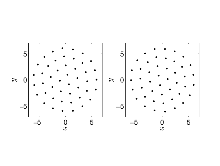
Figure 2: The ground state of the renormalised energy (50) calculated for (a) cω=0.05c_{\omega}=0.05 and (b) cω=0.3c_{\omega}=0.3 with the number of points in each component equal to N=46N=46. Component-1 is shown in the left columns and component-2 in the right columns.
Refer to caption
Figure 3: The critical value of Ωt​s\Omega^{ts} as a function of Γ12\Gamma_{12} calculated analytically by Eq. (55) (solid line) and numerically (dashed line) for the parameters ε=0.0358\varepsilon=0.0358, α1=α2=1\alpha_{1}=\alpha_{2}=1.

We now want to find the ground state of (33) when the radii of both components are equal. Under this condition we have ρ1=ρ2\rho_{1}=\rho_{2}, Γ1=Γ2\Gamma_{1}=\Gamma_{2} and α1=α2\alpha_{1}=\alpha_{2}. This allows us to perform a rescaling that leaves the renormalised energy only dependent on a single parameter. We write Ω=ω​Ωc\Omega=\omega\Omega^{c} for Ωc\Omega^{c} defined in (45). Then

ρ1​(−|log⁡ε|R12+Ωε)=ρ1​|log⁡ε|​(ω​π​Γ2α1​Γ12−1R12)\rho_{1}\left(-\frac{{|\log\varepsilon|}}{R_{1}^{2}}+\frac{\Omega}{\varepsilon}\right)=\rho_{1}{|\log\varepsilon|}\left(\omega\sqrt{\frac{\pi\Gamma_{2}}{\alpha_{1}\Gamma_{12}}}-\frac{1}{R_{1}^{2}}\right) (48)

which implies that we can rescale the pip_{i}’s and qjq_{j}’s as pi=γ​p~ip_{i}=\gamma\tilde{p}_{i} and qj=γ​q~jq_{j}=\gamma\tilde{q}_{j} with

γ2=12​|log⁡ε|​(ω​π​Γ2α1​Γ12−1R12)\gamma^{2}=\frac{1}{2{|\log\varepsilon|}\left(\omega\sqrt{\frac{\pi\Gamma_{2}}{\alpha_{1}\Gamma_{12}}}-\frac{1}{R_{1}^{2}}\right)} (49)

so that the new energy is

12πε2ρ1[−∑i≠jlog|pi−pj|2−∑i≠jlog|qi−qj|2+∑i|pi|2+∑i|qi|2+cω∑i≠j1|pi−qj|2]\frac{1}{2}\pi\varepsilon^{2}\rho_{1}\Bigg[-\sum_{i\neq j}\log|p_{i}-p_{j}|^{2}-\sum_{i\neq j}\log|q_{i}-q_{j}|^{2}\\ +\sum_{i}|p_{i}|^{2}+\sum_{i}|q_{i}|^{2}+c_{\omega}\sum_{i\neq j}\frac{1}{|p_{i}-q_{j}|^{2}}\Bigg] (50)

with

cω=π⁡(1−Γ12)4​α1​Γ122​(2​ω−1)​ε2​|log⁡ε|2.c_{\omega}=\frac{\pi(1-\Gamma_{12})}{4\alpha_{1}\Gamma_{12}^{2}}(2\omega-1)\varepsilon^{2}{|\log\varepsilon|}^{2}. (51)

We simulate this renormalised energy (50) using a conjugate gradient method varying the parameter cωc_{\omega} and the number of vortex points. For a fixed number of lattice points NN, when increasing cωc_{\omega}, the ground state lattice goes from triangular to square at a critical cωt​sc_{\omega}^{ts}. Note that when NN gets large, cωt​sc_{\omega}^{ts} no longer depends on NN. In Fig. 2 we plot the ground state for two values of cωc_{\omega} which give a triangular (cω=0.05c_{\omega}=0.05) and a square lattice (cω=0.3c_{\omega}=0.3) when N=46N=46.

For each NN, we can calculate the critical cωt​sc_{\omega}^{ts} and compare this with the simulations on the full GP equations, as performed in [3] (they provide the appropriate value of NN). From (51), we thus find the critical value of Ω\Omega for which the lattice goes from triangular to square:

Ωt​s=(12+2​cωt​s​α1​Γ122π⁡(1−Γ12)​ε2​|log⁡ε|2)​π​Γ2g1​Γ12​|log⁡ε|\Omega^{ts}=\left(\frac{1}{2}+\frac{2c_{\omega}^{ts}\alpha_{1}\Gamma_{12}^{2}}{\pi(1-\Gamma_{12})\varepsilon^{2}{|\log\varepsilon|}^{2}}\right)\sqrt{\frac{\pi\Gamma_{2}}{g_{1}\Gamma_{12}}}{|\log\varepsilon|} (52)

It turns out that when Ω\Omega gets close to 1, the condensate expands and one has to include in the TF profile a term (1−Ω2)​r2(1-\Omega^{2})r^{2} instead of just r2r^{2}. The radii R1R_{1} and R2R_{2} vary like (1−Ω2)1/4(1-\Omega^{2})^{1/4}. This changes cωc_{\omega} from (51) to

cω=π⁡(1−Γ12)4​α1​Γ122​(2​ω−1−Ω21−Ω2)​ε2​|log⁡ε|2c_{\omega}=\frac{\pi(1-\Gamma_{12})}{4\alpha_{1}\Gamma_{12}^{2}}\left(\frac{2\omega-\sqrt{1-\Omega^{2}}}{\sqrt{1-\Omega^{2}}}\right)\varepsilon^{2}{|\log\varepsilon|}^{2} (53)

so that if we define

βt​s=(12+2​cωt​s​g1​Γ122π⁡(1−Γ12)​|log⁡ε|2)​π​Γ2g1​Γ12​|log⁡ε|\beta_{ts}=\left(\frac{1}{2}+\frac{2c_{\omega}^{ts}g_{1}\Gamma_{12}^{2}}{\pi(1-\Gamma_{12}){|\log\varepsilon|}^{2}}\right)\sqrt{\frac{\pi\Gamma_{2}}{g_{1}\Gamma_{12}}}{|\log\varepsilon|} (54)

then Ωt​s=βt​s​1−(Ωt​s)2\Omega^{ts}=\beta_{ts}\sqrt{1-(\Omega^{ts})^{2}}, which yields

Ωt​s=βt​s1+βt​s2.\Omega^{ts}=\frac{\beta_{ts}}{\sqrt{1+\beta_{ts}^{2}}}. (55)

We plot this form of Ωt​s\Omega^{ts} as a function of Γ12\Gamma_{12} in Fig. 3 where we have taken ε=0.0358\varepsilon=0.0358 and α1=α2=1\alpha_{1}=\alpha_{2}=1 (note that this parameter set corresponds to set ‘ES3’ in [3]). This provides good agreement with simulations of the full Gross Pitaevskii energy and confirms that our point energy (33) well describes the system.

VI Disk Plus Annulus

Equation (29) introduces the critical α¯0\bar{\alpha}_{0} (or equivalently Γ12\Gamma_{12}) for which the two disk state is no longer a solution. In this section we consider α0>α¯0\alpha_{0}>\bar{\alpha}_{0} so that the system is given by a disk in component-1 and an annulus in component-2. This requires α1\alpha_{1} to be different to α2\alpha_{2}, because otherwise the conditions α0>α¯0\alpha_{0}>\bar{\alpha}_{0} and α02−α1​α2≤0\alpha_{0}^{2}-\alpha_{1}\alpha_{2}\leq 0 are not consistent. Defining the inner and outer radii of component-2 to be at r=R2−r=R_{2_{-}} and r=R2+r=R_{2_{+}} such that R2−<R1<R2+R_{2_{-}}<R_{1}<R_{2_{+}}, the appropriate density profiles are

ρT​F,1​(r)=|η1|2=μ1−r22​α1\rho_{TF,1}(r)=|\eta_{1}|^{2}=\frac{\mu_{1}-r^{2}}{2\alpha_{1}} (56)

for 0<r<R2−0<r<R_{2_{-}},

ρT​F,1​(r)=|η1|2\displaystyle\rho_{TF,1}(r)=|\eta_{1}|^{2} =\displaystyle= 12​α1​Γ12​(μ1−α0α2​μ2−r2​Γ2)\displaystyle\frac{1}{2\alpha_{1}\Gamma_{12}}\left(\mu_{1}-\frac{\alpha_{0}}{\alpha_{2}}\mu_{2}-r^{2}\Gamma_{2}\right) (57)
ρT​F,2​(r)=|η2|2\displaystyle\rho_{TF,2}(r)=|\eta_{2}|^{2} =\displaystyle= 12​α2​Γ12​(μ2−α0α1​μ1−r2​Γ1)\displaystyle\frac{1}{2\alpha_{2}\Gamma_{12}}\left(\mu_{2}-\frac{\alpha_{0}}{\alpha_{1}}\mu_{1}-r^{2}\Gamma_{1}\right) (58)

for R2−<r<R1R_{2_{-}}<r<R_{1}, and

ρT​F,2​(r)=|η2|2=μ2−r22​α2\rho_{TF,2}(r)=|\eta_{2}|^{2}=\frac{\mu_{2}-r^{2}}{2\alpha_{2}} (59)

for R1<r<R2+R_{1}<r<R_{2_{+}}.

The normalisation condition (22) gives the following expressions for the radii

R2−\displaystyle R_{2_{-}} =\displaystyle= R−−Γ2Γ1​S\displaystyle\sqrt{R-\sqrt{-\frac{\Gamma_{2}}{\Gamma_{1}}}S} (60)
R1\displaystyle R_{1} =\displaystyle= R−−Γ1Γ2​(1−Γ2)2​S\displaystyle\sqrt{R-\sqrt{-\frac{\Gamma_{1}}{\Gamma_{2}}(1-\Gamma_{2})^{2}}S} (61)
R2+\displaystyle R_{2_{+}} =\displaystyle= R+−Γ1​Γ2​S\displaystyle\sqrt{R+\sqrt{-\Gamma_{1}\Gamma_{2}}S} (62)

and

μ1\displaystyle\mu_{1} =\displaystyle= R\displaystyle R (63)
μ2\displaystyle\mu_{2} =\displaystyle= R+−Γ1​Γ2​S\displaystyle R+\sqrt{-\Gamma_{1}\Gamma_{2}}S (64)

for the chemical potentials. Here we have introduced the parameters

R\displaystyle R =\displaystyle= 2​α~1​(1+α~22α~02​(1−Γ2)2)π\displaystyle 2\sqrt{\frac{\tilde{\alpha}_{1}(1+\frac{\tilde{\alpha}_{2}^{2}}{\tilde{\alpha}_{0}^{2}}(1-\Gamma_{2})^{2})}{\pi}} (65)
S\displaystyle S =\displaystyle= 2​α~1​α~22​(1−Γ2)π​α~02.\displaystyle 2\sqrt{\frac{\tilde{\alpha}_{1}\tilde{\alpha}_{2}^{2}(1-\Gamma_{2})}{\pi\tilde{\alpha}_{0}^{2}}}. (66)

A number of conditions can immediately be found from these expressions. In order for R2−<R1R_{2_{-}}<R_{1}, it must be that Γ12>0\Gamma_{12}>0 [The inequalities R2+>R1R_{2_{+}}>R_{1} and R2+>R2−R_{2_{+}}>R_{2_{-}} are automatically valid]. Secondly, all the expressions (except that for μ1\mu_{1}) require Γ1​Γ2<0\Gamma_{1}\Gamma_{2}<0. This is equivalent to α2>α1\alpha_{2}>\alpha_{1} (under the assumption that the annulus develops in component-2). Thus the range of Γ12\Gamma_{12} for which component-1 is circular and component-2 is annular is given by 0<Γ12<Γ¯120<\Gamma_{12}<\bar{\Gamma}_{12}, where Γ¯12=Γ12\bar{\Gamma}_{12}=\Gamma_{12} evaluated at α0=α¯0\alpha_{0}=\bar{\alpha}_{0} given by (29).

When α0=α¯0\alpha_{0}=\bar{\alpha}_{0} we have shown in Eq. (44) that the critical velocity for creation of the first vortex (that occurs at the origin in component-2) is identically zero. This is precisely the point at which the annulus develops (ρT​F,2​(r=0)=0\rho_{TF,2}(r=0)=0 with R2−=0R_{2_{-}}=0). In the region α0>α¯0\alpha_{0}>\bar{\alpha}_{0}, the first appearance of a topological defect is the development of a giant vortex in component-2 and this can be analyzed fully. We need to introduce

Λ2\displaystyle\Lambda_{2} =α2α2~​∫R2−R2+ρT​F,2​(s)s​𝑑s\displaystyle=\frac{\alpha_{2}}{\tilde{\alpha_{2}}}\int_{R_{2_{-}}}^{R_{2_{+}}}\frac{\rho_{TF,2}(s)}{s}ds (67)
=\displaystyle= 14​α2~​Γ12​[Γ1​R2−2​log⁡(R12R2−2)+Γ12​R2+2​log⁡(R2+2R12)].\displaystyle\frac{1}{4\tilde{\alpha_{2}}\Gamma_{12}}\left[\Gamma_{1}R_{2_{-}}^{2}\log\left({\frac{R_{1}^{2}}{R_{2_{-}}^{2}}}\right)+\Gamma_{12}R_{2_{+}}^{2}\log\left({\frac{R_{2_{+}}^{2}}{R_{1}^{2}}}\right)\right].

Then the critical velocity for nucleation of the giant vortex is determined by Ωg​v=ε​Λ2\Omega_{gv}=\varepsilon\Lambda_{2} and the circulation of this giant vortex is the integer part of Ω/(ε​Λ2)\Omega/(\varepsilon\Lambda_{2}). Next, we want to determine vortices in the bulk and apply (38) to the case of the disk plus annulus. Thus we need to define X2​(r)X_{2}(r) to take into account the giant vortex.

We define X1​(r)X_{1}(r) the primitive of −r​ρT​F,1​(r)-r\rho_{TF,1}(r) which vanishes at R1R_{1} giving

X1​(r)=18​α1​(R12−r2)2+α0​Γ18​α1​α2​Γ12​(R2−2−R12)​(R12+R2−2−2​r2)\begin{split}X_{1}(r)=&\frac{1}{8\alpha_{1}}(R_{1}^{2}-r^{2})^{2}\\ &+\frac{\alpha_{0}\Gamma_{1}}{8\alpha_{1}\alpha_{2}\Gamma_{12}}(R_{2_{-}}^{2}-R_{1}^{2})(R_{1}^{2}+R_{2_{-}}^{2}-2r^{2})\end{split} (68)

for 0<r<R2−0<r<R_{2_{-}}, and is the same as Eq. (35) in the region R2−<r<R1R_{2_{-}}<r<R_{1}. In order to account for the development of vortices beyond the giant vortex, we must recall that additional to the term −εΩ∫rρT​F,2(if2,∇f2)-\varepsilon\Omega\int r\rho_{TF,2}(if_{2},\nabla f_{2}), there will be a kinetic energy term coupling the giant vortex and the vortex cores, namely ε2​d​∫ρT​F,2/r⁡(i​f2,∇f2)\varepsilon^{2}d\int\rho_{TF,2}/r(if_{2},\nabla f_{2}), where dd is the degree of the giant vortex, of order Ω/(ε​Λ2)\Omega/(\varepsilon\Lambda_{2}). Therefore, we define X2​(r)X_{2}(r) to be the primitive of −r​ρT​F,2​(r)+(1/Λ2)​ρT​F,2​(r)/r-r\rho_{TF,2}(r)+(1/\Lambda_{2})\rho_{TF,2}(r)/r which vanishes at both R2−=0R_{2_{-}}=0 and R2+=0R_{2_{+}}=0,

X2​(r)=∫rR2+s​ρT​F,2​(s)​𝑑s−1Λ2​∫rR2+ρT​F,2​(s)s​𝑑sX_{2}(r)=\int_{r}^{R_{2_{+}}}s\rho_{TF,2}(s)d{s}-\frac{1}{\Lambda_{2}}\int_{r}^{R_{2_{+}}}\frac{\rho_{TF,2}(s)}{s}d{s} (69)

where Λ2\Lambda_{2} is given by (67). Completing the integrals gives

X2​(r)=18​α2​(R2+2−r2)2−α0​Γ28​α1​α2​Γ12​(R12−r2)2−14​α2​Γ12​Λ2​(Γ1​R2−2​log⁡(R12r2)CLOSEOPEN+Γ12​R2+2​log⁡(R2+2R12)+Γ1​r2−Γ1​R2−2)\begin{split}X_{2}(r)=&\frac{1}{8\alpha_{2}}(R_{2_{+}}^{2}-r^{2})^{2}-\frac{\alpha_{0}\Gamma_{2}}{8\alpha_{1}\alpha_{2}\Gamma_{12}}(R_{1}^{2}-r^{2})^{2}\\ &-\frac{1}{4{\alpha}_{2}\Gamma_{12}\Lambda_{2}}\Bigg(\Gamma_{1}{R_{2_{-}}^{2}}\log\left(\frac{R_{1}^{2}}{r^{2}}\right)\\ &+\Gamma_{12}{R_{2_{+}}^{2}}\log\left(\frac{R_{2_{+}}^{2}}{{R_{1}^{2}}}\right)+\Gamma_{1}r^{2}-\Gamma_{1}R_{2_{-}}^{2}\Bigg)\end{split} (70)

for R2−<r<R1R_{2_{-}}<r<R_{1} and

X2​(r)=18​α2​(R2+2−r2)2−14​α2​Λ2​(R2+2​log⁡(R2+2r2)+r2−R2+2)\begin{split}X_{2}(r)=&\frac{1}{8\alpha_{2}}(R_{2_{+}}^{2}-r^{2})^{2}\\ &-\frac{1}{4{\alpha}_{2}\Lambda_{2}}\left({R_{2_{+}}^{2}\log\left(\frac{R_{2_{+}}^{2}}{r^{2}}\right)+r^{2}-R_{2_{+}}^{2}}\right)\end{split} (71)

for R1<r<R2+R_{1}<r<R_{2_{+}}.

Refer to caption
Refer to caption
Figure 4: (a) Functions ρT​F,1/X1{\rho_{TF,1}}/{X_{1}} (solid lines) and ρT​F,2/X2{\rho_{TF,2}}/{X_{2}} (dashed lines) given by Eq’s (72)-(75) for Γ12=0.0202\Gamma_{12}=0.0202 (black lines) and Γ12=0.015\Gamma_{12}=0.015 (blue lines). (b) The critical velocity for creation of the first vortex plotted from Eq. (41) [black line] and numerically [blue line] as a function of Γ12\Gamma_{12}. The solid part corresponds to a vortex in component 1 at the center and the dashed part in component 2 in the interface region. The parameters are ε=0.0352\varepsilon=0.0352, α1=0.97\alpha_{1}=0.97 and α2=1.03\alpha_{2}=1.03. Note that Γ¯12=0.02\bar{\Gamma}_{12}=0.02

As before we write down the ratios ρT​F,i/Xi{\rho_{TF,i}}/{X_{i}}:

ρT​F,1X1​(r)=4(R12−r2)−(4​Γ1​α0Γ12​α2​(R2−2−R12)​(R2−2−r2)(R12−r2))×[(R12−r2)2+Γ1​α0Γ12​α2(R2−2−R12)(R12+R2−2−2r2)]−1\begin{split}\frac{\rho_{TF,1}}{X_{1}}(r)=&\frac{4}{(R_{1}^{2}-r^{2})}-\left({\frac{4\Gamma_{1}\alpha_{0}}{\Gamma_{12}\alpha_{2}}\frac{(R_{2_{-}}^{2}-R_{1}^{2})(R_{2_{-}}^{2}-r^{2})}{(R_{1}^{2}-r^{2})}}\right)\\ &\times\Big[(R_{1}^{2}-r^{2})^{2}\\ &+\frac{\Gamma_{1}\alpha_{0}}{\Gamma_{12}\alpha_{2}}(R_{2_{-}}^{2}-R_{1}^{2})(R_{1}^{2}+R_{2_{-}}^{2}-2r^{2})\Big]^{-1}\end{split} (72)

for 0<r<R2−0<r<R_{2_{-}},

ρT​F,1X1​(r)\displaystyle\frac{\rho_{TF,1}}{X_{1}}(r) =\displaystyle= 4(R12−r2),\displaystyle\frac{4}{(R_{1}^{2}-r^{2})}, (73)
ρT​F,2X2​(r)\displaystyle\frac{\rho_{TF,2}}{X_{2}}(r) =\displaystyle= 4​Γ1Γ12​(R2−2−r2)\displaystyle\frac{4\Gamma_{1}}{\Gamma_{12}}(R_{2_{-}}^{2}-r^{2}) (74)
×[(R2+2−r2)2−α0​Γ2α1​Γ12(R12−r2)2\displaystyle\quad\times\Bigg[(R_{2_{+}}^{2}-r^{2})^{2}-\frac{\alpha_{0}\Gamma_{2}}{\alpha_{1}\Gamma_{12}}(R_{1}^{2}-r^{2})^{2}
−2Λ2​Γ12​(Γ1​R2−2​log⁡(R12r2)CLOSE\displaystyle\qquad-\frac{2}{\Lambda_{2}\Gamma_{12}}\Bigg(\Gamma_{1}R_{2_{-}}^{2}\log\left(\frac{R_{1}^{2}}{r^{2}}\right)
+Γ12R2+2log(R2+2R12)+Γ1(r2−R2−2))]−1\displaystyle\qquad+\Gamma_{12}R_{2_{+}}^{2}\log\left(\frac{R_{2_{+}}^{2}}{R_{1}^{2}}\right)+\Gamma_{1}(r^{2}-R_{2_{-}}^{2})\Bigg)\Bigg]^{-1}

for R2−<r<R1R_{2_{-}}<r<R_{1} and

ρT​F,2X2​(r)=4​(R2+2−r2)(R2+2−r2)2−2Λ2​(R2+2​log⁡(R2+2r2)+r2−R2+2)\frac{\rho_{TF,2}}{X_{2}}(r)=\frac{4(R_{2_{+}}^{2}-r^{2})}{(R_{2_{+}}^{2}-r^{2})^{2}-\frac{2}{\Lambda_{2}}\left(R_{2_{+}}^{2}\log\left(\frac{R_{2_{+}}^{2}}{r^{2}}\right)+r^{2}-R_{2_{+}}^{2}\right)} (75)

for R1<r<R2+R_{1}<r<R_{2_{+}}.

It follows that

min⁡(ρT​F,1X1)={4​α2​Γ2​R12+α0​Γ1​R2−2α2​Γ2​R14+α0​Γ1​R2−4for0<r<R2−4(R12−R2−2)forR2−<r<R1.\min\left(\frac{\rho_{TF,1}}{X_{1}}\right)=\begin{cases}4\frac{\alpha_{2}\Gamma_{2}R_{1}^{2}+\alpha_{0}\Gamma_{1}R_{2_{-}}^{2}}{\alpha_{2}\Gamma_{2}R_{1}^{4}+\alpha_{0}\Gamma_{1}R_{2_{-}}^{4}}\quad&\text{for}\qquad 0<r<R_{2_{-}}\\ \frac{4}{(R_{1}^{2}-R_{2_{-}}^{2})}\quad&\text{for}\qquad R_{2_{-}}<r<R_{1}.\end{cases} (76)

Using the expressions above for the radii, we see that

4​α2​Γ2​R12+α0​Γ1​R2−2α2​Γ2​R14+α0​Γ1​R2−4=2α1~​πα2​(α1​α~2+α~1​α2)4\frac{\alpha_{2}\Gamma_{2}R_{1}^{2}+\alpha_{0}\Gamma_{1}R_{2_{-}}^{2}}{\alpha_{2}\Gamma_{2}R_{1}^{4}+\alpha_{0}\Gamma_{1}R_{2_{-}}^{4}}=\frac{2}{\tilde{\alpha_{1}}}\sqrt{\frac{\pi}{\alpha_{2}}\left(\alpha_{1}\tilde{\alpha}_{2}+\tilde{\alpha}_{1}\alpha_{2}\right)} (77)

which we note is independent of α0\alpha_{0}. If we compare the values of Eq. (76), we see that they are equal when α0=α¯0\alpha_{0}=\bar{\alpha}_{0} (which we can consider a degenerate case) and otherwise min⁡(ρT​F,1/X1)\min({\rho_{TF,1}}/{X_{1}}) over the whole space is simply given by the expression in Eq. (77). This implies that the vortex in component-1 is preferred at the origin rather than in the interface region of the two components.

To complete the analysis we must also find the min⁡(ρT​F,2/X2)\min({\rho_{TF,2}}/{X_{2}}) over the whole space to determine whether vortices appear first in component 1 or component 2. It is not possible to find an analytic expression for this minimum and so we must resort to plotting the function and comparing this to min⁡(ρT​F,1/X1)\min({\rho_{TF,1}}/{X_{1}}). In Fig. 4, we plot the functions ρT​F,1/X1{\rho_{TF,1}}/{X_{1}} and ρT​F,2/X2{\rho_{TF,2}}/{X_{2}} in two different cases where min⁡(ρT​F,1/X1)<min⁡(ρT​F,2/X2)\min({\rho_{TF,1}}/{X_{1}})<\min({\rho_{TF,2}}/{X_{2}}) and min⁡(ρT​F,1/X1)>min⁡(ρT​F,2/X2)\min({\rho_{TF,1}}/{X_{1}})>\min({\rho_{TF,2}}/{X_{2}}). We also plot the critical Ω\Omega defined in Eq. (41) as a function of Γ12\Gamma_{12}. We see that until some critical value of Γ12\Gamma_{12}, the vortex first nucleates at the origin in component-1, while above in some small region in Γ12\Gamma_{12} before reaching Γ¯12\bar{\Gamma}_{12}, the vortex first nucleates in the interface region in the second component. Then, increasing Ω\Omega, leads to a vortex lattice close to this point of nucleation. Recall that the giant vortex is always present.

Conclusion

From the energy of a rotating two component condensate, we have derived a reduced energy (33) governing the location of peaks and vortices. We have found that the ground state of this reduced energy yields a square lattice of vortices in regimes consistent with the ones found numerically for the full Gross Pitaevskii energy. We have analyzed in detail the geometry of the ground state (two disks or disk and annulus) and derived formula of the critical velocity for the appearance of the first vortex. We can determine in which component the first vortex appears and the shape of the lattice.

Acknowledgments

The authors acknowledge support from the French ministry Grant ANR-BLAN-0238, VoLQuan.

References

  • [1] Schweikhard, V et al. 2004. Phys. Rev. Lett. 93, 210403.
  • [2] Kasamatsu, K., Tsubota, M. and Ueda, M. 2005. Int. J. Modern Phy. B 19, 11 (1835-1904).
  • [3] Mason, P. & Aftalion, A. 2011. Phys. Rev. A 84, 033611.
  • [4] Eto, M. et al. 2011. Phys. Rev. A 83, 063603.
  • [5] Mueller, E. J. and Ho, T-L. 2002. Phys. Rev. Lett. 88, 180403.
  • [6] Keçeli, M. and Oktel, Ö. 2006. Phys. Rev. A 73, 023611.
  • [7] Cooper, N. R. 2008. Advances in Physics 57, 539.
  • [8] R.Barnett, G.Rafael, M.A.Porter, H.P.Buchler, New J. Phys. 10, 043030 (2008).
  • [9] Aftalion, A. and Du Q., Phys. Rev A 64 (2001) Vol.6, 063603.
  • [10] Aftalion, A., Vortices in Bose Einstein condensates, Progress in Nonlinear Differential Equations and their Applications, Vol.67 Birkhäuser Boston, Inc., Boston, MA, (2006).
  • [11] Y.Castin & R.Dum, Eur. Phys. J. D, 7, 399 (1999).
  • [12] A.L.Fetter, Rev. Mod. Phys. 81, 647 (2009).
  • [13] L. Lassoued, P. Mironescu, Ginzburg–Landau type energy with discontinuous constraint, J. Anal. Math. 77 (1999) 1–26.
  • [14] T.C. Lin, J. Wei, Half-Skyrmions and Spike-Vortex Solutions of Two-Component Nonlinear Schrödinger Systems, J. Math. Phys. 48, 053518 (2007).