Towards the fast scrambling conjecture

There is a growing consensus based on evidence from string theory and gauge-gravity correspondences that black holes do not destroy information when they evaporate. Roughly, the argument is that black holes can be realized in string theory in a manner that accounts for their entropy [1, 2, 3, 4, 5, 6, 7], and that certain string theories are equivalent to manifestly unitary systems [8, 9, 10]. For a recent review, see [11].

Instead of being lost, information about the microscopic state of the black hole leaks out with the hole’s Hawking radiation, much as it would for any other radiating object. Early estimates for the amount of time it would take to recover a bit from a black hole, however, suggested that no information would leak out for an amount of time proportional to the black hole lifetime [12, 13, 14]. Since astrophysical black holes have lifetimes many orders of magnitude longer than the age of the universe, that is tantamount to the information being lost forever. More specifically, such a long delay before the escape of information provided a plausible resolution to some of the conceptual conundrums of quantum gravity, most notably the apparent inconsistency of information release with the quantum no-cloning principle [14].

More recent estimates using techniques from quantum information theory, on the other hand, suggest that information could be released from black holes much more quickly [15]. Those calculations indicate that the relevant time scale is not the amount of time it takes for the black hole to evaporate but, instead, the amount of time the dynamics takes to “scramble” the black hole’s microscopic degrees of freedom in such a way that initially localized perturbations become undetectable by observables that fail to probe a significant fraction of all the degrees of freedom. While a direct calculation of this scrambling time remains out of reach, the relaxation timescales associated with classical black holes are incredibly fast. So fast, in fact, that if they also govern the scrambling time, then the black hole complementarity principle, one of the guiding principles for many researchers in quantum gravity [14, 16, 17] is only just saved from inconsistency – faster scrambling would lead to a paradox.

Motivated by these considerations, as well as the implications of the existence of fast scramblers for the underlying structure of the degrees of freedom of quantum gravity, Sekino and Susskind elaborated on the speculations of [15] to formulate the following three-part fast scrambling conjecture [18, 19]:

1. 1.

   The most rapid scramblers take a time logarithmic in the number of degrees of freedom.

2. 2.

   Matrix quantum mechanics (systems whose degrees of freedom are $n$ by $n$ matrices) saturate the bound.

3. 3.

   Black holes are the fastest scramblers in nature.

The purpose of this article is to explore the validity of the conjecture, focusing primarily on the first part. While the conjecture implicitly refers to the most rapid scramblers in nature, we allow ourselves the freedom to investigate the most rapid scramblers in quantum mechanics (and even slightly beyond) without worrying if our models are physically realizable.

Thanks to earlier research in quantum computation by Dankert et al., it is already known how to define a time-dependent Hamiltonian which will scramble in logarithmic time with high probability [20]. The scrambler, however, is a very carefully engineered quantum circuit, so that it is difficult to ascribe the fast scrambling specifically to interactions between the constituents as opposed to clever tuning of their external knobs. Ideally, therefore, we would like to exhibit a fast scrambler described by a simple time-independent Hamiltonian. To that end, we present two examples:

• •

  Brownian quantum circuits. The scrambler of [20] was a highly structured quantum circuit. Other work has studied circuits composed of random gates [21, 22, 23, 24, 25] but a rigorous proof that they scramble in logarithmic time remains to be found. Instead, we present a continuous-time analog of a quantum circuit in which the Hamiltonian is a stochastically varying two-body interaction, and prove that it scrambles in logarithmic time.

• •

  Ising model. We consider scrambling by the antiferromagnetic Ising interaction on a general graph with an external field parallel to the spin quantization axis. Despite its triviality, this model nonetheless exhibits a form of weak scrambling in logarithmic time on some graphs.

The careful reader will have observed that neither of these examples meets all of our criteria for a convincing scrambler: the Brownian quantum circuits are time-dependent, if not structured, and the Ising model fails to scramble fully. Nonetheless, we feel that, taken together, the examples provide substantial evidence that quantum systems with simple time-independent Hamiltonians can scramble in logarithmic time.

The fast scrambling conjecture not only states that logarithmic-time scramblers exist, but also asserts that it is impossible to scramble faster. It might seem hopeless to address this question without invoking additional physical assumptions beyond just the validity of quantum mechanics. After all, scrambling is a form of information propagation, and limits on information propagation normally depend on locality. A Hamiltonian allowing all degrees of freedom to interact directly has no locality to speak of. Nonetheless, using bounds of Lieb-Robinson-type [26, 27, 28] to rigorously control a mean-field approximation, we are able to show the following:

• •

  Subject to some nontrivial norm assumptions on the terms in the Hamiltonian, no physical system described by a Hamiltonian with dense two-body interactions can scramble in time faster than $O({\log n})$, where $n$ is the number of degrees of freedom.¹¹ 1 Throughout the article, $O(f(n))$ is used in the physicist’s sense of “leading order”. Readers familiar with asymptotic notation should for the most part reinterpret these expressions as $\Theta(f(n))$. “Dense” here means that the number of interacting pairs of degrees of freedom scales like $O(n^{2})$.

• •

  The bound extends to certain four-body Hamiltonians similar to the BFSS matrix model [8].

• •

  With more sparsely interacting systems, there is a lower bound of $O(\sqrt{\log n})$ on the scrambling time.

While the norm assumptions are unfortunately too stringent to allow us to apply the results rigorously to the matrix model Hamiltonian and, thereby, to black hole physics, these results are strong evidence that scrambling in less than logarithmic time is impossible. (A related obstacle is our focus on distinguishable degrees of freedom; bosonic degrees of freedom naturally lead to unbounded operators.)

Scrambling is nothing other than a strong form of thermalization applicable to closed system evolution. A closed system never forgets its initial state, but over time it might become impossible to distinguish different initial states without measuring a large fraction of all the system degrees of freedom. The minimum time required for the information about the initial state to be lost is called the scrambling time.

In general, the scrambling time depends on the nature of the set of initial states. For example, small perturbations of an equilibrium configuration will generally get scrambled more rapidly than will a pair of metastable configurations. Likewise, it could be easier to scramble a discrete set of states than all possible superpositions of those states. In this article, we will focus on product initial states, but a slightly different formulation will likely be necessary in order to study black hole physics. In particular, energy conservation will usually prohibit the strong form of scrambling we demand here.²² 2 A general definition of scrambling appropriate to finite temperature will be included in an upcoming revision of this article.

Suppose that we have a system with $n$ distinguishable degrees of freedom and a Hamiltonian $H=\sum_{\langle x,y\rangle}H_{\langle x,y\rangle}$ acting on a Hilbert space ${\cal H}={\cal H}_{1}\otimes{\cal H}_{2}\otimes\cdots\otimes{\cal H}_{n}$, where the sum ranges over pairs $\langle x,y\rangle$ of degrees of freedom. An initial state $|\Psi(0)\rangle$ evolves to a state $|\Psi(t)\rangle=\exp(-iHt)|\Psi(0)\rangle$. For $S\subseteq\{1,2,\ldots,n\}$ a subset of the degrees of freedom and $S^{c}$ the complement, let $\Psi_{S}(t)=\operatorname{tr}_{S^{c}}|\Psi(t)\rangle\!\langle\Psi(t)|$.

Ideally, a scrambler will delocalize any information initially localized with respect to the factorization of ${\cal H}$ into subsystems. We therefore define the scrambling time $t_{*}$ to be smallest time $t$ such that $\Psi_{S}(t)\simeq\Phi_{S}(t)$ for all $S$ such that $|S|<\kappa n$ for some $0<\kappa<1/2$, and for all initial states $|\Psi(0)\rangle$ and $|\Phi(0)\rangle$ that factorize into the form $|\omega_{1}\rangle\otimes|\omega_{2}\rangle\otimes\cdots\otimes|\omega_{n}\rangle$. For concreteness, we will fix $\kappa=1/3$, but its specific value will not affect our conclusions.

The scrambling time obviously depends on the normalization of the Hamiltonian. In Sekino and Susskind’s original formulation, the fast scrambling conjecture was that $t_{*}/\beta\geq C(\beta)\log n$, where $\beta$ is the inverse temperature and $C$ is an unspecified function. In much of what follows, we will work either far from equilibrium, where $\beta$ is not be well-defined, or near infinite temperature, where it doesn’t accurately reflect the energy per degree of freedom (which stays finite as $\beta\rightarrow 0$ in the spin models we consider). This leaves a couple of alternatives for a dimensionless measure of scrambling time:

• •

  One can consider the ratio of the amount of time it takes to scramble systems of different sizes, hopefully cancelling the temperature dependence. Let $t_{*}^{(k)}$ be the scrambling time for subsystems of size $|S|\leq k$ and set $\tau_{*}=t_{*}^{(\kappa n)}/t_{*}^{(1)}$. The revised conjecture is then that $\tau_{*}\geq O(\log n)$.

• •

  The Hamiltonians we consider do not have their interactions arranged in a lattice structure. Instead, each subsystem $S$ generally participates in a number of interactions growing with $n$. As a second option, one can require that the energy scales extensively with the system size $n$, thereby selecting a normalization for the Hamiltonian which, while coarse, is sufficient to determine the scaling of $t_{*}$ with $n$.

The final step in formalizing the notion of scrambling time is to clarify the meaning of $\Psi_{S}(t)\simeq\Phi_{S}(t)$. The trace distance provides a notion of statistical distinguishability that meshes well with the quantum information theoretic applications of scrambling. Specifically, one should demand that $\|\Psi_{S}(t)-\Phi_{S}(t)\|_{*}<\epsilon$ where $\|X\|_{*}=\operatorname{tr}\sqrt{X^{\dagger}X}$. (See, e.g., [46] for a discussion of the statistical interpretation of the norm.)

A quantum circuit is an idealized model of the time evolution of a quantum computer, which is generally assumed to consist of a number of qubits. At a given discrete time step, a collection of “gates” is applied to the state, where a gate is a unitary transformation involving one or two qubits. Each qubit participates in at most one gate per time step.

As mentioned earlier, Dankert et al. found a quantum circuit that scrambles $n$ qubits after $O(\log n)$ time steps [20]. Their circuit, however, is quite an intricate construction that doesn’t plausibly model any naturally occurring interactions. Other researchers have studied random quantum circuits, establishing that they are scramblers, but the question of whether they scramble in time $O(\log n)$ remains open [21, 22, 23, 24, 25].

In this section, we study a continuous-time analog of a random quantum circuit, which provably does scramble in time $O(\log n)$. Consider $n$ qubits interacting according to a stochastically varying Hamiltonian. Time is subdivided into steps of length $\epsilon=\Delta t$ and during a given time step, the interaction between each pair of qubits is given by a random Wigner matrix. More formally, the Hamiltonian from time $t_{r}=r\Delta t$ to $t_{r+1}=(r+1)\Delta t$ is given by

where the $\Delta B_{r,j,k,\alpha_{j},\alpha_{k}}$ are independent and identically chosen real Gaussians $N(0,\epsilon^{2})$ with zero mean and variance $\epsilon^{2}$ . The operator $\sigma_{j}^{\alpha_{j}}$ represents the Pauli operator $\sigma^{\alpha_{j}}$ acting on qubit $j$, with $\sigma^{0}$ the identity matrix.

The time evolution from $t_{0}$ to $t_{r}$ is given by

For this process to have a well-defined and nontrivial limit as $\Delta t\rightarrow 0$, one must choose $\epsilon^{2}\propto(\Delta t)^{-1}$ [48]. That is, the strength of the interactions must increase as the size of the time steps decreases. This requirement makes it problematic to interpret $t_{*}$ in units of energy. Instead, we show that the ratio $\tau_{*}=t_{*}^{(\kappa n)}/t_{*}^{(1)}=O(\log n)$ for constant $0<\kappa<1/2$. More generally, the ratio of the time required to scramble systems of size $k$ to the time required to scramble a single qubit scales like $O(\log k)$.

The limiting dynamics of the random Hamiltonian evolution is given by $U(0)=I$ and $U(t+dt)=\exp(i\,dG(t))\,U(t)$ for

where the $dB_{j,k,\alpha_{j},\alpha_{k}}(t)$ are independent Brownian motions with unit variance per unit time. Since we are only interested in $\tau_{*}$, the normalization factor is of no real consequence; it is chosen such that $\|dG(t)\|^{2}_{2}=dt$.

Calculating using the Ito calculus (see [49] for an accessible introduction) leads to the following stochastic differential equation for $U(t)$:

(In a slight abuse of notation, we henceforth write $dB_{\alpha_{j},\alpha_{k}}(t):=dB_{j,k,\alpha_{j},\alpha_{k}}(t)$. $I_{\setminus\{j,k\}}$ denotes the identity on all sites except for $i$ and $j$.) Suppose we have some initial state $|\Psi(0)\rangle$. Then the state $\Psi(t)=U(t)|\Psi(0)\rangle\langle\Psi(0)|U^{\dagger}(t)$ undergoes the dynamics

The time evolution will have scrambled subsystem $S$ once $\Psi_{S}(t)$ is independent of the initial state, as measured by the trace distance as discussed in Section 2. Equivalently, $\Psi_{S}(t)$ should approach a fixed state independent of $\Psi(0)$. In the case of Brownian circuits, that fixed state is close to maximally mixed provided $S$ is not too large. Rather than calculating $\|\Psi_{S}(t)-I_{S}/\dim{\cal H}_{S}\|_{1}$ directly, it is much easier to evaluate

An application of Cauchy-Schwarz ensures that if $\operatorname{tr}\Psi_{S}(t)^{2}<(1+\epsilon^{2})/\dim{\cal H}_{S}$, then $\|\Psi_{S}(t)-I_{S}/\dim{\cal H}_{S}\|_{1}<\epsilon$, as required for scrambling.

We therefore introduce the purity of a subsystem $S$:

The equation of motion for the purity $h_{S}(t)$ is given by

After some algebra, it is shown in Appendix A that (11) gives the following dynamics for the purity averaged over realizations of the Brownian motion, $\overline{h}_{S}=\mathbb{E}_{B}[h_{S}]$:

Here $|A|$ means log dim $A$. If the initial configuration $\Psi(0)$ consists of a pure product state, then $\overline{h}_{S}$ depends only on $|S|=k$, so the system of ODE’s collapses to a tridiagonal system and can be written in the form

The rough features of the system (13) are sketched in Figure 1 and the system’s behavior is studied in Appendix B, with the conclusion that the ratio scrambling time

There is an inherent difficulty in searching for fast scramblers: the intuition that a given system will rapidly scramble information is usually based on a sense that the dynamics is complicated, which is almost invariably an obstacle to studying the details of the system’s time evolution. Complexity is not an absolute requirement, however. In this section, we will see that one of the simplest conceivable quantum mechanical systems has lessons to teach us about scrambling time.

Let $G=(V,E)$ be an undirected graph. Assign a spin-$\frac{1}{2}$ to each vertex $v\in V$ and allow spins adjacent with respect to the edge set $E$ to interact via the antiferromagnetic Ising Hamiltonian

as illustrated in Figure 2.

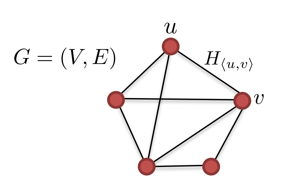
The normalization factor $|V|/|E|$ is chosen to ensure that the energy per spin scales extensively with the system size, $n=|V|$, as discussed in Section 2. Choosing $|0_{z}\rangle$ and $|1_{z}\rangle$ to be the $+1$ and $-1$ eigenstates of $\sigma^{z}$, the Hamiltonian can be written more simply as

The system obviously can’t scramble because any product state of the form $|i_{1}^{z}\rangle|i_{2}^{z}\rangle\cdots|i_{n}^{z}\rangle$ is an eigenstate of $H$. Local information encoded in that basis remains locally accessible for all times. On the other hand, information in the conjugate basis of $\sigma^{x}$ eigenstates, $|0^{x}\rangle$ and $|1^{x}\rangle$, potentially has more interesting behavior. Suppose then that the initial state is $|\Psi(0)\rangle=|i_{1}^{x}\rangle|i_{2}^{x}\rangle\cdots|i_{n}^{x}\rangle$.

Up to a global phase, the system is periodic with period $\pi|E|/|V|$ and the state $|\Psi(t)\rangle$ at time $t$ is most entangled at time $t_{\operatorname{ent}}=\pi|E|/(2|V|)$. The state $|\Psi(t_{\operatorname{ent}})\rangle$ is known as a graph state in quantum computation, where it plays a central role in the measurement-based quantum computing architecture [50, 51]. For a subset $S\subseteq V$ of spins, the entanglement entropy of the density operator $\Psi_{S}(t_{\operatorname{ent}})=\operatorname{tr}_{S^{c}}|\Psi(t_{\operatorname{ent}})\rangle\!\langle\Psi(t_{\operatorname{ent}})|$ has a simple formula in terms of the submatrix $\operatorname{Adj}_{S}$ of the adjacency matrix of $G$ that selects the rows of $S$ and the columns of $S^{c}$ [52]:

where the entropy is measured in bits. It follows that if $\operatorname{Adj}_{S}$ has full rank as a matrix over ${{\mathbb{Z}}}_{2}$, then the entanglement is $|S|$ bits. The only density operator with $|S|$ bits of entropy on $|S|$ qubits, however, is the maximally mixed density operator. Therefore, if $\operatorname{Adj}_{S}$ has rank $|S|$, the final density operator on $S$ will be independent of the choice of initial state $|\Psi(0)\rangle=|i_{1}^{x}\rangle\cdots|i_{n}^{x}\rangle$. That is, the system will have scrambled the $\sigma^{x}$ eigenstates.

Each edge from $S$ to $S^{c}$ contributes a nonzero entry to $\operatorname{Adj}_{S}$, but formula (17) implies that too many connections can reduce entanglement. For example, for the fully connected graph, every row of $\operatorname{Adj}_{S}$ is just a sequence of ones, so there is never more than one bit of entanglement entropy. To maximize the entanglement between $S$ and $S^{c}$, one needs the matrix $\operatorname{Adj}_{S}$ to have full rank for all $|S|\leq n/2$. This is generically the case for appropriate random graphs in which edges are included randomly and independently in $G$ according to the rule $\operatorname{Pr}[(u,v)\in E]=p$.

Since $t_{\operatorname{ent}}=\pi|E|/n$, minimizing $t_{\operatorname{ent}}$ requires minimizing the expected number of edges in the graph, which is ${n\choose 2}p$, subject to the constraint that the rank of $\operatorname{Adj}_{S}$ be maximal for all $|S|\leq n/2$. As $n$ goes to infinity and $\frac{|S|}{|S^{c}|}$ goes to any constant $\alpha$, the rank defect of the matrix is Poisson distributed with parameter $\alpha e^{-\gamma}$ provided $(\log n+\gamma)/n\leq p\leq 1-(\log n+\gamma)/n$ [53]. Therefore, $\operatorname{Adj}_{S}$ will be full rank with probability at least $1-e^{-\gamma}$. Thus, the minimal value of $t_{\operatorname{ent}}$ is equal to $\pi(\log n+\gamma)$, where $\gamma$ can be regarded as a constant.

Even though the system doesn’t scramble fully in the sense of making all local information locally inaccessible, it does scramble the basis of $\sigma^{x}$ eigenstates and does so in time logarithmic in $n$, as required of a fast scrambler.

For the sake of comparison with the Brownian circuit model, it is also instructive to consider the analog of $\tau_{*}$, the ratio of the amount of time to scramble systems of size $\kappa n$ to the time required to scramble a single qubit. Since the system is exactly solvable, it is straightforward to establish by direct calculation that for $S=\{j\}$ a singleton, the Hamiltonian (16) and initial state $|\Psi(0)\rangle$ imply

where $d_{j}$ is the number of graph neighbors of site $j$. The expected number of neighbors per site is $p(n-1)$. Requiring that (18) be close to minimal, i.e. $\frac{1}{2}$, gives the 1-scrambling time as $O(\sqrt{pn})=O(\sqrt{\log n})$. The ratio of the times required for scrambling $\sigma^{x}$ eigenstates therefore scales like $O(\sqrt{\log n})=O(\log n/\sqrt{\log n})$. This hints at the possibility that for systems that do scramble all product states, unlike this Ising model, $\tau_{*}$ might also fail obey an $\Omega(\log n)$ lower bound as required by the fast scrambling conjecture.

Regardless, the Ising model provides an example of a system capable of producing large scale multipartite entanglement sufficient to scramble all information stored locally in a fixed basis on a time scale no more than logarithmic with the number of degrees of freedom.

One way to prove lower bounds on the scrambling time is to exploit the connection between scrambling and signalling. In particular, scrambling a subsystem $S$ implies the ability to signal to the complementary subsystem $S^{c}$. The main task of this section is therefore to prove signalling bounds, but we must do so without relying on relativity or, more generally, any underlying geometry in the organization of the degrees of freedom. Our technique goes back to Lieb and Robinson [26], who proved bounds on commutators $[O_{A}(t),O_{B}]$ for observables $O_{A}$ and $O_{B}$ localized on subsystems $A$ and $B$ of lattice spin systems. To signal reliably from $B$ to $A$, there must be normalized observables for which the norm of the commutator is $O(1)$. Hastings improved the original Lieb-Robinson technique so as to produce dimension-independent bounds [54] and Nachtergaele-Sims showed how to adapt it to general graphs [27]. The version we start from combines both features and is due to Hastings and Koma [28].

As we will see, the Lieb-Robinson technique gives lower bounds on the time required to signal from $B$ to $A$ provided $A$ and $B$ are both constant-sized subsystems. The definition of scrambling used in this paper, however, only implies signalling from a constant-sized $B$ to the complementary subsystem $S^{c}$, and $S^{c}$ will generally involve at least half the degrees of freedom in the whole system. To deal with this large $S^{c}$, we use the Lieb-Robinson bound to show that a mean-field approximation to the time evolution remains reasonably good for sufficiently short times, provided the initial state has product form. For as long as the mean-field approximation holds, the dynamics cannot generate any significant entanglement, which prohibits signalling to $S^{c}$ and, of course, scrambling.

References

- (1) L. Susskind, Some speculations about black hole entropy in string theory, hep-th/9309145.
- (2) A. Sen, Extremal black holes and elementary string states, Mod.Phys.Lett. A10 (1995) 2081–2094, [hep-th/9504147].
- (3) A. Strominger and C. Vafa, Microscopic origin of Bekenstein-Hawking entropy, Phys.Lett. B379 (1996) 99–104, [hep-th/9601029].
- (4) C. G. Callan and J. M. Maldacena, D-brane approach to black hole quantum mechanics, Nucl. Phys. B472 (1996) 591–610, [hep-th/9602043].
- (5) S. R. Das and S. D. Mathur, Excitations of D strings, entropy and duality, Phys.Lett. B375 (1996) 103–110, [hep-th/9601152].
- (6) J. M. Maldacena and L. Susskind, D-branes and fat black holes, Nucl.Phys. B475 (1996) 679–690, [hep-th/9604042].
- (7) G. T. Horowitz and J. Polchinski, A correspondence principle for black holes and strings, Phys.Rev. D55 (1997) 6189–6197, [hep-th/9612146].
- (8) T. Banks, W. Fischler, S. Shenker, and L. Susskind, M theory as a matrix model: A conjecture, Phys.Rev. D55 (1997) 5112–5128, [hep-th/9610043].
- (9) J. Maldacena, The large limit of superconformal field theories and supergravity, Advances in theoretical and mathematical physics 2 (1998) 231–252, [hep-th/9711200].
- (10) J. Maldacena, Eternal black holes in anti-de Sitter, Journal of High Energy Physics 04 (2003) 021, [hep-th/0106112].
- (11) V. Balasubramanian and B. Czech, Quantitative approaches to information recovery from black holes, Classical and quantum gravity 28 (2011) 163001.
- (12) D. N. Page, Average entropy of a subsystem, Phys.Rev.Lett. 71 (1993) 1291, [gr-qc/9305007].
- (13) D. N. Page, Black hole information, in Proceedings of the 5th Canadian conference on general relativity and relativistic astrophysics (R. B. Mann and R. G. McLenaghan, eds.), 1993. hep-th/9305040.
- (14) L. Susskind, L. Thorlacius, and J. Uglum, The stretched horizon and black hole complementarity, Phys.Rev. D48 (1993) 3743, [hep-th/9306069].
- (15) P. Hayden and J. Preskill, Black holes as mirrorrs: quantum information in random subsystems, Journal of high energy physics 09 (2007) 120, [0708.4025].
- (16) Y. Kiem, H. Verlinde, and E. Verlinde, Black hole horizons and complementarity, Phys.Rev. D52 (1995) 7053–7065, [hep-th/9502074].
- (17) D. A. Lowe, J. Polchinski, L. Susskind, L. Thorlacius, and J. Uglum, Black hole complementarity versus locality, Phys.Rev. D52 (Dec., 1995) 6997–7010, [hep-th/9506138].
- (18) Y. Sekino and L. Susskind, Fast scramblers, Journal of High Energy Physics 10 (2008) 065, [0808.2096].
- (19) L. Susskind, Addendum to fast scramblers, 1101.6048.
- (20) C. Dankert, R. Cleve, J. Emerson, and E. Livine, Exact and approximate unitary 2-designs and their application to fidelity estimation, Phys.Rev. A80 (2009), no. 1 012304, [quant-ph/0606161].
- (21) J. Emerson, E. Livine, and S. Lloyd, Convergence conditions for random quantum circuits, Phys.Rev. A72 (2005), no. 6 060302, [quant-ph/0503210].
- (22) A. W. Harrow and R. A. Low, Random quantum circuits are approximate 2-designs, Comm.Math.Phys. 291 (2009) 257–302, [0802.1919].
- (23) L. Arnaud and D. Braun, Efficiency of producing random unitary matrices with quantum circuits, Phys.Rev. A78 (2008), no. 6 062329, [arXiv:0807.0775].
- (24) W. G. Brown and L. Viola, Convergence rates for arbitrary statistical moments of random quantum circuits, Phys.Rev.Lett. 104 (2010), no. 25 250501, [0910.0913].
- (25) I. T. Diniz and D. Jonathan, Comment on the paper “Random quantum circuits are approximate 2-designs”, Comm.Math.Phys. 304 (2011) 281–293, [1006.4202].
- (26) E. H. Lieb and D. W. Robinson, The finite group velocity of quantum spin systems, Comm.Math.Phys. 28 (1972) 251–257.
- (27) B. Nachtergaele and R. Sims, Lieb-Robinson bounds and the exponential clustering theorem, Comm.Math.Phys. 265 (2006) 119–130, [math-ph/0506030].
- (28) M. B. Hastings and T. Koma, Spectral gap and exponential decay of correlations, Comm.Math.Phys. 265 (2006) 781–804, [math-ph/0507008].
- (29) C. Asplund, D. Berenstein, and D. Trancanelli, Evidence for fast thermalization in the BMN matrix model, Phys.Rev.Lett. 107 (2011) 171602, [arXiv:1104.5469].
- (30) J. L. F. Barbon and J. M. Magan, Chaotic fast scrambling at black holes, arXiv:1105.2581.
- (31) K. Schoutens, H. Verlinde, and E. Verlinde, Quantum black hole evaporation, Phys.Rev. D48 (1993) 2670–2685, [hep-th/9304128].
- (32) J. von Neumann, Proof of the ergodic theorem and the H-theorem in quantum mechanics, The European Physical Journal H 35 (2010) 201–237. Original: Zeitschrift für Physik 57, 30 (1929).
- (33) J. Gemmer, M. Michel, and G. Mahler, Quantum thermodynamics, vol. 784 of Lecture Notes in Physics. Springer-Verlag, Berlin, second ed., 2009. Emergence of thermodynamic behavior within composite quantum systems.
- (34) N. Linden, S. Popescu, A. J. Short, and A. Winter, Quantum mechanical evolution towards thermal equilibrium, Phys.Rev. E79 (2009), no. 6 061103, 12, [arXiv:0812.2385].
- (35) S. Goldstein, J. L. Lebowitz, R. Tumulka, and N. Zanghì, Canonical typicality, Phys.Rev.Lett. 96 (2006), no. 5 050403, 3.
- (36) S. Popescu, A. J. Short, and A. Winter, Entanglement and the foundations of statistical mechanics, Nat. Phys. 2 (2006), no. 11 754–758, [quant-ph/0511225v3].
- (37) P. Reimann, Foundation of statistical mechanics under experimentally realistic conditions, Phys.Rev.Lett. 101 (Nov, 2008) 190403.
- (38) P. Bocchieri and A. Loinger, Ergodic foundation of quantum statistical mechanics, Phys.Rev. (2) 114 (1959) 948–951.
- (39) S. Lloyd, Black Holes, Demons, and the Loss of Coherence. PhD thesis, Rockefeller University, 1988.
- (40) H. Tasaki, From quantum dynamics to the canonical distribution: general picture and a rigorous example, Phys.Rev.Lett. 80 (1998), no. 7 1373–1376.
- (41) P. Calabrese and J. Cardy, Time dependence of correlation functions following a quantum quench, Phys.Rev.Lett. 96 (2006), no. 13 136801, [cond-mat/0601225].
- (42) J. M. Deutsch, Quantum statistical mechanics in a closed system, Phys.Rev. A43 (Feb, 1991) 2046–2049.
- (43) M. Srednicki, Chaos and quantum thermalization, Phys.Rev. E50 (Aug, 1994) 888–901, [cond-mat/9403051].
- (44) A. Riera, C. Gogolin, and J. Eisert, Thermalization in nature and on a quantum computer, arXiv:1102.2389.
- (45) M. Rigol and M. Srednicki, Alternatives to eigenstate thermalization, arXiv:1108.0928.
- (46) M. A. Nielsen and I. L. Chuang, Quantum Computation and Quantum Information. Cambridge University Press, 2000.
- (47) M. Fannes, A continuity property of the entropy density for spin lattice systems, Comm.Math.Phys. 31 (1973) 291–294.
- (48) I. Karatzas and S. E. Shreve, Brownian motion and stochastic calculus. Springer, 1991.
- (49) L. Arnold, Stochastic differential equations: theory and applications. Dover, 1974.
- (50) R. Raussendorf, D. E. Browne, and H. J. Briegel, Measurement-based quantum computation on cluster states, Phys.Rev. A68 (2003), no. 2 022312, [quant-ph/0301052].
- (51) M. van den Nest, A. Miyake, W. Dür, and H. J. Briegel, Universal resources for measurement-based quantum computation, Phys.Rev.Lett. 97 (2006), no. 15 150504, [quant-ph/0604010].
- (52) M. Hein, J. Eisert, and H. J. Briegel, Multiparty entanglement in graph states, Phys.Rev. A69 (2004), no. 6 062311, [quant-ph/0307130].
- (53) V. F. Kolchin, Random graphs. Cambridge University Press, 1999.
- (54) M. B. Hastings, Lieb-Schultz-Mattis in higher dimensions, Phys.Rev. B69 (2004), no. 10 104431, [cond-mat/0305505].
- (55) P. Hayden and A. Winter, The fidelity alternative and quantum identification, . arXiv:1003.4994.
- (56) P. Hayden, M. Horodecki, A. Winter, and J. Yard, A decoupling approach to the quantum capacity, Open systems and information dynamics 15 (2008) 7–19, [quant-ph/0702005].
- (57) B. Nachtergaele, H. Raz, B. Schlein, and R. Sims, Lieb-Robinson bounds for harmonic and anharmonic lattice systems, Comm.Math.Phys. 286 (2009) 1073–1098, [arXiv:0712.3820].