跳到论文正文
W Papers独立论文阅读器 arXiv:1111.6402 论文正文 计算阅读时间 · 0%
引用这篇论文根据当前论文元数据生成,正式投稿前建议核对。


License: arXiv.org perpetual non-exclusive license
arXiv:1111.6402v2 [hep-ph] 27 Mar 2012

November 2011

FCNC portals to the dark sector

Jernej F. Kamenik1,2,11 1 jernej.kamenik@ijs.si and Christopher Smith3,22 2 c.smith@ipnl.in2p3.fr

1J. Stefan Institute, Jamova 39, P. O. Box 3000, 1001 Ljubljana, Slovenia
2Department of Physics, University of Ljubljana, Jadranska 19, 1000 Ljubljana, Slovenia

3Université Lyon 1 & CNRS/IN2P3, UMR5822 IPNL, Rue Enrico Fermi 4, 69622 Villeurbanne Cedex, France

Abstract

The most general basis of operators parametrizing a low-scale departure from the SM particle content is constructed. The SM gauge invariance is enforced, and operators of lowest dimensions are retained separately for a new light neutral particle of spin 0, 1/2, 1, and 3/2. The basis is further decomposed into couplings to the SM Higgs/gauge fields, to pairs of quark/lepton fields, and to baryon/lepton number violating combinations of fermion fields. This basis is then used to systematically investigate the discovery potential of the rare FCNC decays of the KK and BB mesons with missing energy in the final state. The most sensitive decay modes in the s→ds\to d, b→db\to d, and b→sb\to s sectors are identified and compared for each type of couplings to the new invisible state.


1 Introduction

Though extremely successful, the Standard Model (SM) is not expected to be valid up to arbitrary high energies. It certainly needs to be amended at the Planck scale, with the advent of quantum gravity. But then, some new dynamics should show up already at a much lower scale, though still above the electroweak scale, to avoid hierarchy problems. With this picture in mind, it seems natural to assume that all the New Physics (NP) degrees of freedom are heavier than the known SM particles, and decouple at low energy. In a fully model-independent way, the impact on the SM of any NP model can then be embedded into non-renormalizable effective operators, under the provision that these involve only the SM fields and satisfy the SM gauge symmetries. The full classification of these operators has been achieved many years ago, by Buchmuller and Wyler [1] for the baryon- and lepton-number conserving operators, and by Weinberg [2] for those violating these global symmetries.

Still, whether the SM particles are the only dynamical degrees of freedom within the electroweak energy range is far from established. Not only is the existence of new light particles not excluded, since they would evade direct detection when sufficiently weakly interacting, but their presence could even be welcome. Indeed, many NP models are built upon some spontaneously broken symmetries, and do often have remnants at low-energy in the form of massless or very light Goldstone bosons. A well-known example is the axion [3], introduced to cure the strong CP problem of the SM. More crucially, there are now very strong indications that the universe is filled with dark matter, so there should be at least one new electrically neutral colorless particle, possibly lighter than the electroweak scale. Once opening that door, it is not such a drastic step to imagine a whole dark sector, i.e. a full-fledged set of darkly interacting dark particles only loosely connected to our own visible sector. Further, it should be stressed that adjoining a dark sector to the SM is always possible, does not need to be directly related to dark matter (so one would rather speak of a hidden sector), and is actually quite generic in supersymmetric models. For a recent review, including further physical motivations from string theory or extra dimensional settings, see e.g. Ref. [4].

In the present work, our main goal is to construct the lowest-dimensional effective interactions parametrizing a low-scale departure from the SM particle content. Specifically, we assume that there is a new particle of spin 00, 1/21/2, 11, or 3/23/2, neutral under the SM gauge group S​U​(3)C⊗S​U​(2)L⊗U​(1)YSU(3)_{C}\otimes SU(2)_{L}\otimes U(1)_{Y}, and write down the gauge invariant operators coupling this particle to SM fields. These effective interactions are not yet included and thus complement the NP operator basis of Refs. [1, 2]. To our knowledge, such a complete basis has never been presented, though parts of it already appeared in the literature. In particular, those effective couplings between SM and dark particles which are renormalizable, sometimes called portals, have already been investigated [5].

Our second goal is to constrain the effective operators. Since the new state is assumed neutral under the SM gauge group, it looks like a natural dark matter candidate. However, the viability of this hypothesis would require constraining its mass, couplings, and lifetime, and this in general requires more inputs about the dark sector dynamics. Here, we refrain from doing so and rather concentrate exclusively on the quark FCNC transitions s→d​Xs\to dX, b→d​Xb\to dX, and b→s​Xb\to sX, where XX collectively denotes any final state made of dark particles. Our focus on these modes, instead of for example leptonic observables or collider signals, is motivated on one hand by their extreme sensitivities to NP (as detailed in the next section), and on the other, by the next generation of experiments currently under construction. Indeed, rare KK decays are the main targets of the NA62 (CERN) and K0TO (J-Parc) experiments, while rare BB decays could be accessed at the Super-B (Italy) and Belle II (KEK) facilities. So, in the present work, we further assume that the dark particle is light enough to be directly produced in KK and/or BB meson decays, and sufficiently long-lived to escape detection in flavor factories. For all practical matters, this new particle is invisible, and would show up as missing energy in FCNC-induced rare KK and BB decays (for recent works along this line, see e.g. Refs. [6, 7]).

Our analysis is organized according to the dark particle spin. To keep the discussion focused on the operator basis, we rely on extensive appendices to cover the issues of hadronic matrix elements and differential rates. So, before entering the discussion, the next section summarizes the main features of the observables considered here, i.e. the rare KK and BB decays. Then, given our focus on FCNC processes, a flavor-based classification of the dark operators is described in the following section, on which we rely throughout the paper.

Rare FCNC decays

The FCNC-induced decay modes are very suppressed in the SM, where the missing energy is carried away by a ν​ν¯\nu\bar{\nu} pair (see Fig. 1). So, even relatively small NP contributions could be evidenced. Specifically, to set the stage and get an idea of the sensitivity of the rare KK and BB decays, imagine that a NP operator of dimension nn contributes to dI→dJ​Xd^{I}\to d^{J}X, with I=2,3I=2,3, J=1,2J=1,2 the quark generation indices. If its Wilson coefficient is set to one, then there is a scale Λ\Lambda such that the NP contribution equates the SM prediction for dI→dJ​ν​ν¯d^{I}\to d^{J}\nu\bar{\nu},

mIn−6Λn−4≈g2MW2​g216​π2​|Vt​I∗​Vt​J|,\frac{m_{I}^{n-6}}{\Lambda^{n-4}}\approx\frac{g^{2}}{M_{W}^{2}}\frac{g^{2}}{16\pi^{2}}|V_{tI}^{\ast}V_{tJ}|\;, (1)

with m2,3=mK,Bm_{2,3}=m_{K,B}, gg the S​U​(2)LSU(2)_{L} coupling constant, and VV the CKM matrix. As shown in Table 1 as a function of the dimension, the SM loop factor combined with the CKM suppression pushes the scales Λ\Lambda well above the electroweak scale for n≲7n\lesssim 7. On the contrary, the rare decay constraints cease to make sense for S​U​(2)L⊗U​(1)YSU(2)_{L}\otimes U(1)_{Y} invariant operators of dimension n≳9n\gtrsim 9, since powers of (H†​H)/Λ2→v2/Λ2(H^{\dagger}H)/\Lambda^{2}\to v^{2}/\Lambda^{2} grow unchecked when Λ≲v\Lambda\lesssim v, where v≈246v\approx 246 GeV is the SM Higgs vacuum expectation value.

Refer to caption
Figure 1: The rare decays with missing energy in the SM, as induced by the Z penguin (W boxes are understood).
n=5n=5 n=6n=6 n=7n=7 n=8n=8 n=9n=9
s→ds\to d 3.3⋅1073.3\cdot 10^{7} TeV 130130 TeV 2.02.0 TeV 0.250.25 TeV 0.070.07 TeV
b→db\to d 1.3⋅1051.3\cdot 10^{5} TeV 2626 TeV 1.51.5 TeV 0.370.37 TeV 0.160.16 TeV
b→sb\to s 2.7⋅1042.7\cdot 10^{4} TeV 1212 TeV 0.90.9 TeV 0.250.25 TeV 0.110.11 TeV
Table 1: Naive reach, in terms of scales Λ\Lambda and as a function of the effective operator dimension nn, of the rare FCNC-induced KK and BB decays, as estimated from Eq. (1) with the CKM values of Eq. (6).

Clearly, these scales are only indicative. The true sensitivity to a given dark operator depends essentially on two additional factors. First, the quark transitions dI→dJ​Xd^{I}\to d^{J}X have to be probed through hadronic processes. Hence, depending on the modes, hadronic matrix elements as well as phase-space factors can alter significantly the estimates of Table 1. In the following, we compare the sensitivities of all the leading modes. Specifically, in the KK sector, we include the modes with the least number of pions and photons in the final states, i.e. K→XK\to X, K→π​XK\to\pi X, K→γ​XK\to\gamma X, and K→π​π​XK\to\pi\pi X, and leave out the K→π​π​π​XK\to\pi\pi\pi X modes. Similarly, in the BB sector, the considered modes are the B→XB\to X, B→(K,K∗)​XB\to(K,K^{\ast})X, and B→(π,ρ)​XB\to(\pi,\rho)X decay channels. The γ​X\gamma X channel, driven in the KK sector by the QED anomaly, is suppressed and difficult to reconstruct experimentally in the BB sector, and will thus not be included [6].

The second factor determining the true sensitivity of a given mode is related to the experimental strategies deployed to measure it. Since invisible states are not seen, the kinematical reconstruction is limited. In addition, these modes are so rare (in the SM) that they require very aggressive background suppressions. To this end, the central tool is the differential rate in terms of the kinematical parameters of the visible products. But this differential rate depends on the nature of the dark particle. Currently, most experimental analyses implicitly impose the SM differential rate (for X=ν​ν¯X=\nu\bar{\nu}). This means that the current bounds cannot be directly translated to other types of final state particles. This motivates another goal of the present paper, which is to provide the full dictionary of the differential rates for all the leading effective interactions involving invisible final states. These spectra should be used by the experimentalists to derive bounds for each type of new invisible state.

For more details on these issues, including kinematics, matrix elements, current measurements or bounds, and experimental prospects for the various modes, we refer to appendix A.1 (B.1) for KK (BB) decays.

Flavor-based classification of the dark operators

At the electroweak scale, once the whole NP particle spectrum but the XX has been integrated out, the lowest dimensional operators can be split into three types according to their quark and lepton field contents:

ℋe​f​f=ℋm​a​t+ℋi​n​t+ℋΔ​ℬ,Δ​ℒ.\mathcal{H}_{eff}=\mathcal{H}_{mat}+\mathcal{H}_{int}+\mathcal{H}_{\Delta\mathcal{B},\Delta\mathcal{L}}\;. (2)

By definition, ℋi​n​t\mathcal{H}_{int} contains only gauge and Higgs fields, while ℋm​a​t\mathcal{H}_{mat} and ℋΔ​ℬ,Δ​ℒ\mathcal{H}_{\Delta\mathcal{B},\Delta\mathcal{L}} contain at least one SM fermionic field. The operators of ℋΔ​ℬ,Δ​ℒ\mathcal{H}_{\Delta\mathcal{B},\Delta\mathcal{L}} have a non-zero charge under the baryon (ℬ\mathcal{B}) or lepton (ℒ\mathcal{L}) number U⁡(1)U(1)s. As in Ref. [1, 2], all the operators are to be written as manifestly invariant under S​U​(3)C⊗S​U​(2)L⊗U​(1)YSU(3)_{C}\otimes SU(2)_{L}\otimes U(1)_{Y}, i.e. in terms of the quark (lepton) doublets QQ (L)(L) and singlets U,DU,D (E)(E) of each flavor, of the S​U​(3)C,S​U​(2)L,U​(1)YSU(3)_{C},SU(2)_{L},U(1)_{Y} field strengths Gμ​νa,Wμ​νi,Bμ​νG_{\mu\nu}^{a},W_{\mu\nu}^{i},B_{\mu\nu}, of the Higgs doublet HH, as well as of covariant derivatives acting on these fields, insofar as these cannot be reduced using the SM equations of motion (EOM).

Due to their different field contents, these three types of operators do not contribute equally to the quark transitions s→d​Xs\to dX, b→d​Xb\to dX, and b→s​Xb\to sX, so let us organize them differently, in terms of four classes of scenarios, as shown in Table 2.

Consider first the operators of ℋm​a​t\mathcal{H}_{mat} involving down-type quarks (those with leptons or up-type quarks are obtained by substituting D,Q→E,LD,Q\to E,L or D,H→U,H∗D,H\to U,H^{\ast}). Up to possible partial derivatives acting on the quark or invisible fields, and omitting the Dirac structures, the quark currents are

ℋm​a​t=cR​LI​JΛn​H†​D¯I​QJ×X+cL​RI​JΛn​H​Q¯I​DJ×X+cL​LI​JΛn​Q¯I​QJ×X+cR​RI​JΛn​D¯I​DJ×X.\mathcal{H}_{mat}=\dfrac{c_{RL}^{IJ}}{\Lambda^{n}}H^{\dagger}\bar{D}^{I}Q^{J}\times X+\frac{c_{LR}^{IJ}}{\Lambda^{n}}H\bar{Q}^{I}D^{J}\times X+\dfrac{c_{LL}^{IJ}}{\Lambda^{n}}\bar{Q}^{I}Q^{J}\times X+\dfrac{c_{RR}^{IJ}}{\Lambda^{n}}\bar{D}^{I}D^{J}\times X\;. (3)

Those operators have a flavor structure, and thus can in principle induce dI→dJ​Xd^{I}\to d^{J}X. Clearly, when analyzing the physics reach of rare KK and BB decays in terms of the scale Λ\Lambda, the assumptions made on the cI≠Jc^{I\neq J} are crucial. There are two main scenarios:

  • I.

    The constraints derived from rare FCNC decays are the tightest when the NP flavor structure is generic,

    cI≠J∼𝒪⁡(1).c^{I\neq J}\sim\mathcal{O}(1)\;. (4)

    As shown in Table 1, the bounds on the NP scale Λ\Lambda are then often far above the electroweak scale.

  • II.

    Since ℋm​a​t\mathcal{H}_{mat} results from integrating out the whole NP particle spectrum, the flavor-breaking character of its operators could originate from dynamical effects not related to the dark sector. In that case, the NP dynamics would also quite naturally correct the visible FCNC operators, on which there are many tight experimental constraints from KK and BB physics [8]. This is typically the case in supersymmetric settings, where the flavored soft-breaking terms cannot be fully generic. Phenomenologically, a simple way to account for such a non-generic NP flavor structure is to impose the Minimal Flavor Violation (MFV) ansatz [9], i.e. force the quark currents to have the forms

    D¯I​(𝐘d​𝐘u†​𝐘u)I​J​QJ,Q¯I​(𝐘u†​𝐘u)I​J​QJ,D¯I​(𝐘d​𝐘u†​𝐘u​𝐘d†)I​J​DJ.\bar{D}^{I}(\mathbf{Y}_{d}\mathbf{Y}_{u}^{\dagger}\mathbf{Y}_{u})^{IJ}Q^{J}\;,\;\;\bar{Q}^{I}(\mathbf{Y}_{u}^{\dagger}\mathbf{Y}_{u})^{IJ}Q^{J}\;,\;\bar{D}^{I}(\mathbf{Y}_{d}\mathbf{Y}_{u}^{\dagger}\mathbf{Y}_{u}\mathbf{Y}_{d}^{\dagger})^{IJ}D^{J}\;. (5)

    In the down-quark mass-eigenstate basis, the diagonal v​𝐘d=2​𝐦dv\mathbf{Y}_{d}=\sqrt{2}\mathbf{m}_{d} tunes the chirality flips, while v​𝐘u=2​𝐦u​Vv\mathbf{Y}_{u}=\sqrt{2}\mathbf{m}_{u}V parametrizes the flavor change (𝐦u,d\mathbf{m}_{u,d} denotes the diagonal quark mass matrices, VV the CKM matrix, and v≈246v\approx 246 GeV the Higgs vacuum expectation value). So, MFV rescales the Wilson coefficients according to cR​LI​J=mdI​cL​LI​J/vc_{RL}^{IJ}=m_{d}^{I}c_{LL}^{IJ}/v, cL​RI​J=cL​LI​J​mdJ/vc_{LR}^{IJ}=c_{LL}^{IJ}m_{d}^{J}/v, cR​RI​J=mdI​mdJ​cL​LI​J/v2c_{RR}^{IJ}=m_{d}^{I}m_{d}^{J}c_{LL}^{IJ}/v^{2}, and

    cL​LI≠J∼λI​J=𝐘u†​𝐘u≈Vt​I∗​Vt​J→{λs​d≈(−3.1+i​1.3)×10−4,λb​d≈(7.8−i​3.1)×10−3,λb​s≈(−4.0−i​0.07)×10−2.c_{LL}^{I\neq J}\sim\lambda^{IJ}=\mathbf{Y}_{u}^{\dagger}\mathbf{Y}_{u}\approx V_{tI}^{\ast}V_{tJ}\to\left\{\begin{array}[c]{l}\lambda^{sd}\approx(-3.1+i1.3)\times 10^{-4}\;,\\ \lambda^{bd}\approx(7.8-i3.1)\times 10^{-3}\;,\\ \lambda^{bs}\approx(-4.0-i0.07)\times 10^{-2}\;.\end{array}\right. (6)

    Upon these rescalings, the accessible scales Λ\Lambda are then much lower, especially for operators of low dimensions, and for s→ds\to d operators involving light right-handed quarks.

If the whole NP dynamics is flavor blind, then XX couples only to the flavor-diagonal quark currents and cI≠J=0c^{I\neq J}=0. A flavor transition is of course still possible but it must proceed through the SM weak interactions, i.e. the flavor-blind quark currents must be dressed by a flavor-changing WW interaction, either between the quark lines or as a self-energy on these quark lines.

In particular, all the operators of ℋi​n​t\mathcal{H}_{int} are of this type. Indeed, to contribute to FCNC processes, gauge fields have to be coupled to quarks, while Higgs fields are either coupled to quarks or left as external tadpoles (to be replaced by the vacuum expectation value after the electroweak symmetry breaking). The resulting couplings between quarks and XX can then be matched onto ℋm​a​t\mathcal{H}_{mat}, and satisfy11 1 The contributions to cI≠Jc^{I\neq J} are tiny because, as long as the S​U​(2)L⊗U​(1)YSU(2)_{L}\otimes U(1)_{Y} symmetry is exact, the gauge/Higgs fields of the ℋi​n​t\mathcal{H}_{int} operators can couple to a flavor-changing quark current only at the cost of at least two Yukawa insertions, i.e. two Higgs tadpoles, on the quark line. At the high scale, these tadpoles cost a factor Λ−2\Lambda^{-2} compared to the flavor-blind version of the same operator. When Λ\Lambda is large, flavor-changing effects thus dominantly originate from electroweak scale GIM breaking, even though this necessitates an extra WW loop (see Table 2). cI≠J≈0c^{I\neq J}\approx 0. Thus, the only difference with respect to the flavor-blind ℋm​a​t\mathcal{H}_{mat} operators is that the cI​Ic^{II} coefficients are initially suppressed by some power of the SM coupling constants (at the scale Λ\Lambda), by some loop factors, and by quark Yukawa couplings when a Higgs field is coupled to the quark line (so that c33≫c11,22c^{33}\gg c^{11,22}).

For reasons entirely pertaining to the SM dynamics, it is different to probe the couplings to heavy quarks, c33c^{33}, and to light quarks, c11,22c^{11,22}, so these constitute our third and fourth classes of scenarios.

  • III.

    Let us assume we have an operator coupling XX to the top quark current. Dressing it with a WW exchange (see Table 2), the necessary GIM breaking arises at the electroweak scale. From the rare decay perspective, this electroweak physics is local, so it can be matched onto the flavor-changing operators of Class II. The Wilson coefficients end up suppressed by the MFV scalings (6) and by a loop and gauge coupling, i.e.

    cI≠J∼c33​kI​J,kI​J=g216​π2​λI​J→{ks​d≈(−0.8+i​0.4)×10−6,kb​d≈(2.1−i​0.8)×10−5,kb​s≈(−1.1−i​0.02)×10−4.c^{I\neq J}\sim c^{33}k^{IJ}\;,\;\;k^{IJ}=\frac{g^{2}}{16\pi^{2}}\lambda^{IJ}\to\left\{\begin{array}[c]{l}k^{sd}\approx(-0.8+i0.4)\times 10^{-6}\;,\\ k^{bd}\approx(2.1-i0.8)\times 10^{-5}\;,\\ k^{bs}\approx(-1.1-i0.02)\times 10^{-4}\;.\end{array}\right. (7)

    Typically, the bounds on the scale Λ\Lambda are brought down very significantly, often at around the electroweak scale. Still, the rare KK and BB decays remain ideal probes for such kind of effective couplings since a direct collider signal in the t​t¯t\bar{t} channel is presumably hidden by the large flavor-blind SM backgrounds.

  • IV.

    With XX coupled to the light quarks (uu, dd, or ss), it is much trickier to derive bounds on the scale Λ\Lambda for three reasons. Firstly, BB physics is unable to provide competitive constraints, given the small CKM factors Vu​b∗​Vu​sV_{ub}^{\ast}V_{us} or Vu​b∗​Vu​dV_{ub}^{\ast}V_{ud}. Secondly, though in the KK sector the weak transition is favored by the large Vu​s∗​Vu​dV_{us}^{\ast}V_{ud} for CP-conserving observables22 2 CP-violating observables, for which Im⁡(Vu​s∗​Vu​d)=0\operatorname{Im}(V_{us}^{\ast}V_{ud})=0 (this standard CKM convention is used throughout the paper, see e.g. Ref. [10]), are induced by heavy quarks and fall into Class III. Due to the scaling (7), they are very suppressed., the light quarks are never integrated out and remain dynamical. This renders the theoretical control difficult since the KK physics scale is too low to allow for a perturbative QCD treatment. This is true both for the effective operators describing the weak transition and for the effective operators describing the production of the new invisible states. Thirdly, there are already many constraints on the flavor blind production of invisible particles, in particular from π0\pi^{0} or quarkonium decays. Compared to the other classes, it is a priori not clear whether rare decays offer privileged windows. In the following, we will consider only specific scenarios where competitive bounds can be derived.

ℋe​f​f​(qI→qJ​X)=cI​JΛn​q¯I​qJ×X\mathcal{H}_{eff}(q^{I}\to q^{J}X)=\dfrac{c^{IJ}}{\Lambda^{n}_{\;}}\bar{q}^{I}q^{J}\times X
Flavor-violating (cI≠J≠0c^{I\neq J}\neq 0) Flavor-conserving (cI≠J=0c^{I\neq J}=0)
Heavy quark: q=(c),t​q=(c),t\rule{0.0pt}{13.73148pt}\vskip 3.0pt plus 1.0pt minus 1.0pt Light quarks: q=u,d,s,(c)q=u,d,s,(c)
[Uncaptioned image] [Uncaptioned image] [Uncaptioned image]
Bounds on cI​J/Λnc^{IJ}/\Lambda^{n} directly derived from the dI→dJ​Xd^{I}\to d^{J}X processes. When MFV holds, cI​J∼Vt​I∗​Vt​Jc^{IJ}\sim V_{tI}^{\ast}V_{tJ} times the appropriate chirality flip factors mdI,J/vm_{d^{I,J}}/v, see Eq. (6). Same local operator basis, but with the coefficients rescaled as cI​J→(g/(4​π))2​Vt​I∗​Vt​J×c33c^{IJ}\to(g/(4\pi))^{2}V_{tI}^{\ast}V_{tJ}\times c^{33} times the appropriate chirality flip factors mdI,J/vm_{d^{I,J}}/v, see Eq. (7). Due to the small Vu​b∗V_{ub}^{\ast}, BB decays are not competitive. For KK decays, the q=uq=u contributions are dominant but non local, and require controlling long-distance hadronic effects.
Class I, II Class III Class IV
Table 2: Flavor-based classification of the operators involving dark particles, collectively denoted XX. After the electroweak symmetry breaking, the ℋm​a​t\mathcal{H}_{mat} operators are directly matched onto ℋe​f​f​(qI→qJ​X)\mathcal{H}_{eff}(q^{I}\to q^{J}X) and split into the four classes. The ℋi​n​t\mathcal{H}_{int} operators collapse onto the Class III and/or IV flavor-blind operators once their gauge/Higgs fields are attached to quarks. The ℋΔ​ℬ,Δ​ℒ\mathcal{H}_{\Delta\mathcal{B},\Delta\mathcal{L}} operators have different signatures, and do not fit in this classification. Note that the charm quark is considered heavy (light) for KK (BB) decays.

The final type of operators is a bit different and does not immediately fit in the above classification. First, in general, Δ​ℬ\Delta\mathcal{B} and Δ​ℒ\Delta\mathcal{L} dark operators cannot be present simultaneously, since an XX exchange would induce proton decay. A way out would be to impose MFV, which forces Δ​ℒ\Delta\mathcal{L} operators to be proportional to the tiny neutrino masses [11], rendering them irrelevant. The Δ​ℬ\Delta\mathcal{B} operators are not particularly suppressed under MFV, but they never contribute to the FCNC-induced rare decays considered here. Indeed, these modes trivially conserve ℬ\mathcal{B} since an odd number of baryons would be required in the final state. This is not possible for KK decays, while the signatures for BB decays should be experimentally clear, but are beyond our scope.

If MFV is not imposed and Δ​ℬ\Delta\mathcal{B} operators are somehow disposed of, then Δ​ℒ\Delta\mathcal{L} contributions to the dI→dJ​Xd^{I}\to d^{J}X processes are possible. But, the only Δ​ℒ≠0\Delta\mathcal{L}\neq 0 invisible final states either involve an odd number of neutrinos, or some Δ​ℒ=2\Delta\mathcal{L}=2 neutrino pairs νL​νL\nu_{L}\nu_{L}. Since a neutrino field in an effective operator costs Λ−3/2\Lambda^{-3/2}, these are in general significantly suppressed compared to the operators of ℋm​a​t\mathcal{H}_{mat} and ℋi​n​t\mathcal{H}_{int}. The only exceptions are those contributing to dI→dJ​νL​ψd^{I}\to d^{J}\nu_{L}\psi or dI→dJ​νL​Ψd^{I}\to d^{J}\nu_{L}\Psi. As will be discussed in the relevant sections, because νL\nu_{L} is part of the lepton doublet, these operators are always accompanied by the charge-current transitions dI→uJ​ℓ−​ψd^{I}\to u^{J}\ell^{-}\psi or dI→uJ​ℓ−​Ψd^{I}\to u^{J}\ell^{-}\Psi, which may offer better windows than the rare FCNC transitions.

2 Invisible spin-1/2 fermion

When the new invisible fermion is neutral under the SM gauge group and is produced in pairs, imposing the S​U​(3)C⊗S​U​(2)L⊗U​(1)YSU(3)_{C}\otimes SU(2)_{L}\otimes U(1)_{Y} gauge invariance reduces the basis to the usual ten chiral currents:

ℋm​a​tψ¯​ψ\displaystyle\mathcal{H}_{mat}^{\mathrm{\bar{\psi}\psi}} =cL​LVΛ2​Q¯​γμ​Q×ψ¯L​γμ​ψL+cL​RVΛ2​Q¯​γμ​Q×ψ¯R​γμ​ψR+cR​LVΛ2​D¯​γμ​D×ψ¯L​γμ​ψL+cR​RVΛ2​D¯​γμ​D×ψ¯R​γμ​ψR\displaystyle=\frac{c_{LL}^{V}}{\Lambda^{2}}\bar{Q}\gamma_{\mu}Q\times\bar{\psi}_{L}\gamma^{\mu}\psi_{L}+\frac{c_{LR}^{V}}{\Lambda^{2}}\bar{Q}\gamma_{\mu}Q\times\bar{\psi}_{R}\gamma^{\mu}\psi_{R}+\frac{c_{RL}^{V}}{\Lambda^{2}}\bar{D}\gamma_{\mu}D\times\bar{\psi}_{L}\gamma^{\mu}\psi_{L}+\frac{c_{RR}^{V}}{\Lambda^{2}}\bar{D}\gamma_{\mu}D\times\bar{\psi}_{R}\gamma^{\mu}\psi_{R}
+cL​RSΛ3H†D¯Q×ψ¯LψR+cL​LSΛ3H†D¯Q×ψ¯RψL+cR​RSΛ3HQ¯D×ψ¯LψR+cR​LSΛ3HQ¯D×ψ¯RψL\displaystyle\;\;\;\;+\frac{c_{LR}^{S}}{\Lambda^{3}}H^{\dagger}\bar{D}Q\times\bar{\psi}_{L}\psi_{R}+\frac{c_{LL}^{S}}{\Lambda^{3}}H^{\dagger}\bar{D}Q\times\bar{\psi}_{R}\psi_{L}+\frac{c_{RR}^{S}}{\Lambda^{3}}H\bar{Q}D\times\bar{\psi}_{L}\psi_{R}+\frac{c_{RL}^{S}}{\Lambda^{3}}H\bar{Q}D\times\bar{\psi}_{R}\psi_{L}
+cL​LTΛ3H†D¯σμ​νQ×ψ¯Rσμ​νψL+cR​RTΛ3HQ¯σμ​νD×ψ¯Lσμ​νψR,\displaystyle\;\;\;\;+\frac{c_{LL}^{T}}{\Lambda^{3}}H^{\dagger}\bar{D}\sigma_{\mu\nu}Q\times\bar{\psi}_{R}\sigma^{\mu\nu}\psi_{L}+\frac{c_{RR}^{T}}{\Lambda^{3}}H\bar{Q}\sigma_{\mu\nu}D\times\bar{\psi}_{L}\sigma^{\mu\nu}\psi_{R}\;, (8)

with the definition σμ​ν≡i⁡(γμ​γν+gμ​ν)\sigma^{\mu\nu}\equiv i(\gamma^{\mu}\gamma^{\nu}+g^{\mu\nu}), and where QQ (DD) stands for the left-handed quark doublet (right-handed down-quark singlet). Similar operators can be written down for the up-quark right-handed singlet or for leptonic transitions, and the generalization to a two Higgs-doublet model is straightforward.

The coefficients are not assumed real, and their flavor indices are understood. For example, written in full for the s→ds\to d, b→sb\to s, and b→db\to d sectors which concern us here:

cL​LVΛ2​Q¯​γμ​Q×ψ¯L​γμ​ψL≡cL​LV,s​dΛ2​s¯​γμ​PL​d×ψ¯L​γμ​ψL+cL​LV,b​sΛ2​b¯​γμ​PL​s×ψ¯L​γμ​ψL+cL​LV,b​dΛ2​b¯​γμ​PL​d×ψ¯L​γμ​ψL+h.c..\frac{c_{LL}^{V}}{\Lambda^{2}}\bar{Q}\gamma_{\mu}Q\times\bar{\psi}_{L}\gamma^{\mu}\psi_{L}\equiv\frac{c_{LL}^{V,sd}}{\Lambda^{2}}\bar{s}\gamma_{\mu}P_{L}d\times\bar{\psi}_{L}\gamma^{\mu}\psi_{L}+\frac{c_{LL}^{V,bs}}{\Lambda^{2}}\bar{b}\gamma_{\mu}P_{L}s\times\bar{\psi}_{L}\gamma^{\mu}\psi_{L}+\frac{c_{LL}^{V,bd}}{\Lambda^{2}}\bar{b}\gamma_{\mu}P_{L}d\times\bar{\psi}_{L}\gamma^{\mu}\psi_{L}+h.c.\;. (9)

There are only two tensor operators because the identity 2​σμ​ν​γ5=i​εμ​ν​α​β​σα​β2\sigma^{\mu\nu}\gamma_{5}=i\varepsilon^{\mu\nu\alpha\beta}\sigma_{\alpha\beta} forbids Q¯​σμ​ν​D×ψ¯R​σμ​ν​ψL\bar{Q}\sigma_{\mu\nu}D\times\bar{\psi}_{R}\sigma^{\mu\nu}\psi_{L} and D¯​σμ​ν​Q×ψ¯L​σμ​ν​ψR\bar{D}\sigma_{\mu\nu}Q\times\bar{\psi}_{L}\sigma^{\mu\nu}\psi_{R}. The dimension-seven operators involving the SM Higgs field are retained because their suppression is only by v/Λv/\Lambda. By contrast, true dimension-seven operators involving an additional derivative are more severely suppressed by mK,B,ψ/Λm_{K,B,\psi}/\Lambda, and are thus not included.

dd KL→X​XK_{L}\to XX Ki→πj​X​XK^{i}\to\pi^{j}XX KL→γ​X​XK_{L}\to\gamma XX Ki→πj​πk​X​XK^{i}\to\pi^{j}\pi^{k}XX Behavior
i,j,…i,j,... L,0L,0 +,++,+ +,+,0+,+,0 L,+,−L,+,- L,0,0L,0,0 in mXm_{X} for
mXmaxm_{X}^{\max} mK/2m_{K}/2 mπ​(CLOSEm_{\pi}\;(exp. cut)) mK/2m_{K}/2 (mK−2​mπ)/2(m_{K}-2m_{\pi})/2 K→π​X​XK\to\pi XX
12\dfrac{1}{2} fX​SfX​P\begin{array}[c]{c}f_{XS}\\ f_{XP}\end{array} 7¯\bar{7} 7474 2424 1919 −- 33 66 55 [Uncaptioned image]
fV​VfV​A\begin{array}[c]{c}f_{VV}\\ f_{VA}\end{array} 66 −- 140140 9898 2828 33 44 −- [Uncaptioned image]
fA​VfA​A\begin{array}[c]{c}f_{AV}\\ f_{AA}\end{array} 66 −372∗\begin{array}[c]{c}-\\ 372^{\ast}\end{array} −- −- −- 1010 2323 1818 −-
fT​TfT~​T\begin{array}[c]{c}f_{TT}\\ f_{\tilde{T}T}\end{array} 7¯\bar{7} −- 1111 99 1111 44 55 22 [Uncaptioned image]
00 gX​Sg_{XS} 6¯\bar{6} 2400024000 72007200 50005000 −- 380380 11001100 910910
gV​VgA​V\begin{array}[c]{c}g_{VV}\\ g_{AV}\end{array} 6 −- 99−\begin{array}[c]{c}99\\ -\end{array} 70−\begin{array}[c]{c}70\\ -\end{array} 20−\begin{array}[c]{c}20\\ -\end{array} 27\begin{array}[c]{c}2\\ 7\end{array} 316\begin{array}[c]{c}3\\ 16\end{array} −13\begin{array}[c]{r}-\\ 13\end{array} [Uncaptioned image]
11 hX​ShX​P\begin{array}[c]{c}h_{XS}\\ h_{XP}\end{array} 8¯\bar{8} 4.54.5 1.61.6 1.31.3 −- 0.30.3 0.50.5 0.40.4 [Uncaptioned image]
32\dfrac{3}{2} fX​SfX​P\begin{array}[c]{c}f_{XS}\\ f_{XP}\end{array} 9¯\bar{9} 0.510.51 0.190.19 0.200.20 −- 0.0400.040 0.0670.067 0.0630.063 [Uncaptioned image]
fV​VfV​A\begin{array}[c]{c}f_{VV}\\ f_{VA}\end{array} 88 −- 0.120.12 0.110.11 0.070.07 0.0140.014 0.0170.017 −- [Uncaptioned image]
fA​VfA​A\begin{array}[c]{c}f_{AV}\\ f_{AA}\end{array} 88 −0.32∗\begin{array}[c]{c}-\\ 0.32^{\ast}\end{array} −- −- −- 0.0270.027 0.0380.038 0.0340.034 −-
fT​SfT​P\begin{array}[c]{c}f_{TS}\\ f_{TP}\end{array} 9¯\bar{9} −- 0.100.10 0.090.09 0.100.10 0.0340.034 0.0390.039 .016∗.021∗\begin{array}[c]{c}.016^{\ast}\\ .021^{\ast}\end{array} [Uncaptioned image]
fT​TfT~​T\begin{array}[c]{c}f_{TT}\\ f_{\tilde{T}T}\end{array} 9¯\bar{9} −- 0.120.12 0.100.10 0.130.13 0.0460.046 0.0530.053 0.0380.038 [Uncaptioned image]
fT~​SfT~​P\begin{array}[c]{c}f_{\tilde{T}S}\\ f_{\tilde{T}P}\end{array} 9¯\bar{9} −- .08∗.10∗\begin{array}[c]{c}.08^{\ast}\\ .10^{\ast}\end{array} .07∗.08∗\begin{array}[c]{c}.07^{\ast}\\ .08^{\ast}\end{array} 0.100.10 0.0390.039 0.0450.045 0.0330.033 [Uncaptioned image]
Table 3: Pair production of invisible states: Scales Λ\Lambda (in TeV) accessible for each operator, assuming 10−1010^{-10} bounds on all the branching ratios. The operator dimensions dd are written with a bar for those involving a Higgs field, and thus a v/Λv/\Lambda factor. For the K→π​X​XK\to\pi XX modes, the differential rates are integrated over the pion momentum window [140,195]∪[211,229][140,195]\cup[211,229] MeV, see App. A.1. The short-hands XS (XP) stand for SS or PS (SP or PP), as appropriate. The quoted mXmaxm_{X}^{\max} are indicative; the bounds are derived for mX=0m_{X}=0 or, if the rate vanishes (signaled by (*)), for mX=100m_{X}=100 MeV. For those which do not vanish, most V−AV-A, S−PS-P, or T−T~T-\tilde{T} degeneracies are lifted when mX≠0m_{X}\neq 0. Still, the dependences of the Λ\Lambdas on mXm_{X} are rather weak. The bounds stay within an order of magnitude of their values at mX=0m_{X}=0, except for mXm_{X} close to the kinematical threshold, where they sharply drop towards zero. This is shown in the last column for K+→π+​ν​ν¯K^{+}\to\pi^{+}\nu\bar{\nu}, where Λ\Lambda (normalized to the value quoted in the table) is plotted against mXm_{X} over the range [0,mπ][0,m_{\pi}].
dd B0→X​XB^{0}\to XX B→π​X​XB\to\pi XX B→ρ​X​XB\to\rho XX B→K​X​XB\to KXX B→K∗​X​XB\to K^{\ast}XX
mXmaxm_{X}^{\max} mB0/2m_{B^{0}}/2 (mB−mπ)/2(m_{B}-m_{\pi})/2 (mB−mρ)/2(m_{B}-m_{\rho})/2 (mB−mK)/2(m_{B}-m_{K})/2 (mB−mK∗)/2(m_{B}-m_{K^{\ast}})/2
1/21/2 fS​S,S​Pf_{SS,SP} 7¯\bar{7} −- 3.23.2 −- 3.0​(4.6)3.0\,(4.6) −-
fP​S,P​Pf_{PS,PP} 7¯\bar{7} 2.72.7 −- 2.12.1 −- 1.7​(4.0)1.7(4.0)
fV​V,V​Af_{VV,VA} 66 −- 1010 5.35.3 9.7​(19)9.7\,(19) 4.3​(15)4.3(15)
fA​Vf_{AV} 66 −- −- 7.67.6 −- 6.2​(21)6.2(21)
fA​Af_{AA} 66 6.2∗6.2^{\ast} −- 7.67.6 −- 6.2​(21)6.2(21)
fT​Tf_{TT} 7¯\bar{7} −- 2.62.6 3.13.1 2.4​(3.7)2.4\,(3.7) 2.7​(6.2)2.7(6.2)
fT~​Tf_{\tilde{T}T} 7¯\bar{7} −- 2.62.6 3.03.0 2.4​(3.7)2.4\,(3.7) 2.6​(6.0)2.6(6.0)
0 gS​Sg_{SS} 6¯\bar{6} −- 8282 −- 75​(140)75(140) −-
gP​Sg_{PS} 6¯\bar{6} 5050 −- 4646 −- 37​(130)37(130)
gV​Vg_{VV} 66 −- 7.27.2 −- 6.8​(13)6.8(13) −-
gA​Vg_{AV} 66 −- −- 4.74.7 −- 3.9​(13)3.9(13)
1 hS​S,S​Ph_{SS,SP} 8¯\bar{8} −- 0.610.61 −- 0.56​(0.79)0.56(0.79) −-
hP​S,P​Ph_{PS,PP} 8¯\bar{8} 0.560.56 −- 0.420.42 −- 0.36​(0.67)0.36(0.67)
3/2 fS​S,S​Pf_{SS,SP} 9¯\bar{9} −- 0.180.18 −- 0.17​(0.22)0.17\,(0.22) −-
fP​S,P​Pf_{PS,PP} 9¯\bar{9} 0.180.18 −- 0.130.13 −- 0.10​(0.19)0.10(0.19)
fV​V,V​Af_{VV,VA} 88 −- 0.150.15 0.100.10 0.14​(0.19)0.14\,(0.19) 0.09​(0.17)0.09(0.17)
fA​Vf_{AV} 88 −- −- 0.120.12 −- 0.11​(0.20)0.11(0.20)
fA​Af_{AA} 88 0.14∗0.14^{\ast} −- 0.120.12 −- 0.11​(0.20)0.11(0.20)
fT​T,T~​Tf_{TT,\tilde{T}T} 9¯\bar{9} −- 0.160.16 0.160.16 0.15​(0.19)0.15\,(0.19) 0.15​(0.24)0.15(0.24)
fT​S,T​Pf_{TS,TP} 9¯\bar{9} −- 0.140.14 0.120.12 0.13​(0.17)0.13\,(0.17) 0.11​(0.18)0.11(0.18)
fT~​Sf_{\tilde{T}S} 9¯\bar{9} −- 0.11∗0.11^{\ast} 0.140.14 0.09∗​(0.12∗)0.09^{\ast}\,(0.12^{\ast}) 0.12​(0.20)0.12(0.20)
fT~​Pf_{\tilde{T}P} 9¯\bar{9} −- 0.13∗0.13^{\ast} 0.140.14 0.11∗​(0.15∗)0.11^{\ast}\,(0.15^{\ast}) 0.12​(0.20)0.12(0.20)
Table 4: Pair production of invisible states: Scales Λ\Lambda (in TeV) accessible for the various operators with present (future) measurements (see App. B.1). The operator dimensions dd are written with a bar for those involving a Higgs field, and thus a v/Λv/\Lambda factor. We assume mX=0m_{X}=0 everywhere, except when the rate vanishes in this limit (indicated by *). Specifically, the B→X​XB\to XX bound on fA​Af_{AA}, the B→π⁡(K)​X​XB\to\pi(K)XX bounds on gTg_{T}, fT​S,T​Pf_{TS,TP}, and the B→K∗​X​XB\to K^{*}XX bounds on gT,V,Ag_{T,V,A} are derived for mX≃2m_{X}\simeq 2 GeV. The behaviors of the scales Λ\Lambda as functions of mXm_{X} are shown for X=ψX=\psi in Fig. 2.

After the electroweak symmetry breaking, the gauge-invariant operators are rewritten in terms of the (pseudo)scalar, (axial)vector, and (pseudo)tensor currents. This minimizes the interferences between the currents in physical observables, since these operators dominantly produce the invisible fermions in different states. The change of basis is

fV​V,V​A\displaystyle f_{VV,VA} =cL​RV±cL​LV±cR​LV+cR​RV4,fS​S,S​P=vΛ​cL​RS±cL​LS±cR​LS+cR​RS4,fT​T,T~​T=vΛ​cR​RT±cL​LT2,\displaystyle=\frac{c_{LR}^{V}\pm c_{LL}^{V}\pm c_{RL}^{V}+c_{RR}^{V}}{4},\;\;f_{SS,SP}=\frac{v}{\Lambda}\frac{c_{LR}^{S}\pm c_{LL}^{S}\pm c_{RL}^{S}+c_{RR}^{S}}{4}\;,\;f_{TT,\tilde{T}T}=\frac{v}{\Lambda}\frac{c_{RR}^{T}\pm c_{LL}^{T}}{2}\;,
fA​V,A​A\displaystyle f_{AV,AA} =cR​RV±cR​LV∓cL​LV−cL​RV4,fP​S,P​P=vΛ​cR​RS±cR​LS∓cL​LS−cL​RS4,\displaystyle=\frac{c_{RR}^{V}\pm c_{RL}^{V}\mp c_{LL}^{V}-c_{LR}^{V}}{4},\;f_{PS,PP}=\frac{v}{\Lambda}\frac{c_{RR}^{S}\pm c_{RL}^{S}\mp c_{LL}^{S}-c_{LR}^{S}}{4}\;, (10)

where fX​Yf_{XY} tunes q¯I​ΓX​qJ×ψ¯​ΓY​ψ\bar{q}^{I}\Gamma_{X}q^{J}\times\bar{\psi}\Gamma_{Y}\psi with ΓV,A,S,P,T,T~=γμ,γμ​γ5,1,γ5,σμ​ν,σμ​ν​γ5\Gamma_{V,A,S,P,T,\tilde{T}}=\gamma^{\mu},\gamma^{\mu}\gamma_{5},1,\gamma_{5},\sigma_{\mu\nu},\sigma_{\mu\nu}\gamma_{5}, and flavor indices are understood. The corresponding differential rates are listed in Appendix A.3 (B.3) for KK (BB) decays, and the physics reach is summarized in Tables 3 (4). Specifically, the entries of these tables are obtained by turning on each fif_{i} in turn, while keeping the others to zero. We do not do this at the level of the cic_{i} in order to minimize the interferences among the NP contributions. The value of each |fi||f_{i}| is set to one for the vector and axial vector currents, and to v/Λv/\Lambda for the others, in order to keep track of the S​U​(2)L⊗U​(1)YSU(2)_{L}\otimes U(1)_{Y} structure of the underlying operators. Since KL,SK_{L,S} are approximate CP eigenstates, the CP phase of the fif_{i} must be kept arbitrary. Effectively, we turn on Im⁡fi\operatorname{Im}f_{i} and Re⁡fi\operatorname{Re}f_{i} to one (or v/Λv/\Lambda) separately, and the tightest bound (largest Λ\Lambda) is indicated in Table 3.

To derive the entries of Tables 3 and 4, specific experimental bounds on the rare decay branching ratios are used, as detailed in App. A.1 (B.1) for KK (BB) decays. Note that the scales Λ\Lambda corresponding to tighter or looser experimental bounds are immediately obtained by a simple rescaling of the numbers in Tables 3 and 4, given the dimensions of the operators (8) and the definitions (10).

Finally, in Fig. 3, we compare the sensitivity of the various KK and BB decay modes for two illustrative examples, cL​LVc_{LL}^{V} and cL​LSc_{LL}^{S}, with and without imposing MFV. In the former case, the coefficients are set to (cL​LV)I​J=λI​J(c_{LL}^{V})^{IJ}=\lambda^{IJ} and (cL​LS)I​J=λI​J​mdI/v(c_{LL}^{S})^{IJ}=\lambda^{IJ}m_{d^{I}}/v, see Eq. (6). Actually, to avoid dragging a relative factor mb/vm_{b}/v, the scales Λ\Lambda are plotted taking a two Higgs doublet model of type II at large tan⁡β=vu/vd\tan\beta=v_{u}/v_{d} (where vuv_{u} and vdv_{d} are the two Higgs vacuum expectation values), so that mb/vd≈1m_{b}/v_{d}\approx 1 and (cL​LS)s​d(c_{LL}^{S})^{sd} is simply suppressed by ms/mbm_{s}/m_{b}. As can be seen in Fig. 3, this chirality flip is expensive in the KK sector, and pulls the K→π​ψ​ψ¯K\to\pi\psi\bar{\psi} constraint an order of magnitude below those from rare BB decays. By contrast, for the vector current, similar constraints are drawn from rare KK and BB decays when MFV is imposed.

Refer to caption
Figure 2: Evolution of the scales Λ\Lambda associated with the pair production of invisible fermions as a function of the fermion mass. The values at mψ=0m_{\psi}=0 correspond to those quoted in Table 4, except for B→ψ​ψ¯B\to\psi\bar{\psi}, given at mψ=2m_{\psi}=2 GeV. Note that these B→(K(∗),ρ,π)​ψ​ψ¯B\to(K^{(\ast)},\rho,\pi)\psi\bar{\psi} bounds assume flat experimental acceptances and full phase-space coverage, which is not true in the present experimental analyses, see App. B.1.
Refer to caption
Figure 3: Scales Λ\Lambda (in TeV) accessible using the rare KK and BB decays, for the vector current cL​LVc_{LL}^{V} and the scalar current cL​LSc_{LL}^{S}. The plots on the right are obtained when MFV is imposed on the Wilson coefficients.

Let us now turn to the operators not involving the SM fermions, but rather the SM gauge and Higgs fields. Using these fields EOM, as well as partial integration and identities like 2​σμ​ν​γ5=i​εμ​ν​α​β​σα​β2\sigma^{\mu\nu}\gamma_{5}=i\varepsilon^{\mu\nu\alpha\beta}\sigma_{\alpha\beta}, the leading operators reduce to

ℋi​n​tψ¯​ψ\displaystyle\mathcal{H}_{int}^{\mathrm{\bar{\psi}\psi}} =cR​LBΛ​Bμ​ν×ψ¯R​σμ​ν​ψL+cL​RBΛ​Bμ​ν×ψ¯L​σμ​ν​ψR+cR​LHΛ​H†​H×ψ¯R​ψL+cL​RHΛ​H†​H×ψ¯L​ψR\displaystyle=\frac{c_{RL}^{B}}{\Lambda}B_{\mu\nu}\times\bar{\psi}_{R}\sigma^{\mu\nu}\psi_{L}+\frac{c_{LR}^{B}}{\Lambda}B_{\mu\nu}\times\bar{\psi}_{L}\sigma^{\mu\nu}\psi_{R}+\frac{c_{RL}^{H}}{\Lambda}H^{\dagger}H\times\bar{\psi}_{R}\psi_{L}+\frac{c_{LR}^{H}}{\Lambda}H^{\dagger}H\times\bar{\psi}_{L}\psi_{R}
+cL​LHΛ2iH†𝒟↔μH×ψ¯LγμψL+cR​RHΛ2iH†𝒟↔μH×ψ¯RγμψR\displaystyle\;\;\;\;+\frac{c_{LL}^{H}}{\Lambda^{2}}iH^{\dagger}\overleftrightarrow{\mathcal{D}}_{\mu}H\times\bar{\psi}_{L}\gamma^{\mu}\psi_{L}+\frac{c_{RR}^{H}}{\Lambda^{2}}iH^{\dagger}\overleftrightarrow{\mathcal{D}}_{\mu}H\times\bar{\psi}_{R}\gamma^{\mu}\psi_{R}
+cR​L,iGΛ3QiG×ψ¯RψL+cL​R,iGΛ3QiG×ψ¯LψR\displaystyle\;\;\;\;+\frac{c_{RL,i}^{G}}{\Lambda^{3}}Q_{i}^{G}\times\bar{\psi}_{R}\psi_{L}+\frac{c_{LR,i}^{G}}{\Lambda^{3}}Q_{i}^{G}\times\bar{\psi}_{L}\psi_{R}
+cR​LH​BΛ3(H†H)Bμ​ν×ψ¯Rσμ​νψL+cL​RH​BΛ3(H†H)Bμ​ν×ψ¯Lσμ​νψR\displaystyle\;\;\;\;+\frac{c_{RL}^{HB}}{\Lambda^{3}}(H^{\dagger}H)B_{\mu\nu}\times\bar{\psi}_{R}\sigma^{\mu\nu}\psi_{L}+\frac{c_{LR}^{HB}}{\Lambda^{3}}(H^{\dagger}H)B_{\mu\nu}\times\bar{\psi}_{L}\sigma^{\mu\nu}\psi_{R}
+cR​LH​WΛ3(H†σiH)Wμ​νi×ψ¯Rσμ​νψL+cL​RH​WΛ3(H†σiH)Wμ​νi×ψ¯Lσμ​νψR,\displaystyle\;\;\;\;+\frac{c_{RL}^{HW}}{\Lambda^{3}}(H^{\dagger}\sigma^{i}H)W_{\mu\nu}^{i}\times\bar{\psi}_{R}\sigma^{\mu\nu}\psi_{L}+\frac{c_{LR}^{HW}}{\Lambda^{3}}(H^{\dagger}\sigma^{i}H)W_{\mu\nu}^{i}\times\bar{\psi}_{L}\sigma^{\mu\nu}\psi_{R}\;, (11)

where 𝒟↔μ=𝒟←μ−𝒟→μ\overleftrightarrow{\mathcal{D}}_{\mu}=\overleftarrow{\mathcal{D}}_{\mu}-\overrightarrow{\mathcal{D}}_{\mu} and QiGQ_{i}^{G} stand for each of the following gauge-invariant combinations of SM fields

QiG=𝒟μ​H†​𝒟μ​H,(H†​H)2,Bμ​ν​Bμ​ν,Wμ​νi​Wiμ​ν,Gμ​νa​Gaμ​ν,Bμ​ν​B~μ​ν,Wμ​νi​W~iμ​ν,Gμ​νa​G~aμ​ν.Q_{i}^{G}=\mathcal{D}^{\mu}H^{\dagger}\mathcal{D}_{\mu}H,\;(H^{\dagger}H)^{2},\;B_{\mu\nu}B^{\mu\nu},\;W_{\mu\nu}^{i}W_{i}^{\mu\nu},\;G_{\mu\nu}^{a}G_{a}^{\mu\nu},\;B_{\mu\nu}\tilde{B}^{\mu\nu},\;W_{\mu\nu}^{i}\tilde{W}_{i}^{\mu\nu},\;G_{\mu\nu}^{a}\tilde{G}_{a}^{\mu\nu}\;. (12)

But for the last three CP-odd combinations, the QiGQ_{i}^{G} monomials are precisely the dimension-four gauge and Higgs couplings of the SM Lagrangian. Operators with partial derivatives acting on ψ\psi are systematically discarded.

The leading dimension-five operators involve either Bμ​νB_{\mu\nu} or H†​HH^{\dagger}H. The Bμ​νB_{\mu\nu} operators effectively assign a (mass-dependent) hypercharge to the invisible fermions, since under partial integration

Bμ​ν×ψ¯R​σμ​ν​ψL=2​i​Bμ×ψ¯R​𝒟↔μ​ψL+2​mψ​Bμ×(ψ¯L​γμ​ψL+ψ¯R​γμ​ψR).B_{\mu\nu}\times\bar{\psi}_{R}\sigma^{\mu\nu}\psi_{L}=2iB^{\mu}\times\bar{\psi}_{R}\overleftrightarrow{\mathcal{D}}_{\mu}\psi_{L}+2m_{\psi}B_{\mu}\times(\bar{\psi}_{L}\gamma^{\mu}\psi_{L}+\bar{\psi}_{R}\gamma^{\mu}\psi_{R})\;. (13)

With mψ/Λ≪1m_{\psi}/\Lambda\ll 1 but otherwise arbitrary, the second term describes millicharged fermions, a scenario to be discussed later on. The H†​HH^{\dagger}H operators effectively correct the ψ\psi mass after the electroweak symmetry breaking, with (setting cL​R,R​LHc_{LR,RL}^{H} to one)

δ​mψ=v2/Λ.\delta m_{\psi}=v^{2}/\Lambda\;. (14)

Taken at face value, naturality would thus prefer Λ>24​(240)\Lambda>24\,(240) TeV if mψ≈δ​mψ<mB/2m_{\psi}\approx\delta m_{\psi}<m_{B}/2 (mK/2)(m_{K}/2), as required to produce these states in rare BB (KK) decays. As seen in Tables 3 and 4, this would push the NP effects from the FCNC operators (8) just beyond accessibility. Of course, these numbers are only indicative, a specific model need not produce these dimension-five operators, and even if generated, a sizeable deviation from naturality cannot be ruled out.

All the other ℋi​n​tψ¯​ψ\mathcal{H}_{int}^{\mathrm{\bar{\psi}\psi}} operators are, for our purpose, only marginally relevant. As explained in Sec. 1, they reduce to the four-fermion operators of Eq. (8) once Higgs and gauge fields are coupled to quarks, with the four-fermion Wilson coefficients obeying the SM scalings (7). For example, the dimension-six operators with H†​𝒟↔μ​HH^{\dagger}\overleftrightarrow{\mathcal{D}}_{\mu}H reduce, after the electroweak symmetry breaking, to an effective ZZ coupling to ψ\psi which can be treated in perfect analogy to the SM ZZ coupling to ν​ν¯\nu\bar{\nu} (see Fig. 1). The rare decays proceed through the flavor-changing hadronic ZZ penguin, and the four-fermion operators scale like cL​L​(R​R)I​J∼g​cL​L​(R​R)H​kI​Jc_{LL(RR)}^{IJ}\sim gc_{LL(RR)}^{H}k^{IJ} with kI​Jk^{IJ} given in Eq. (7).

The final class of operators involves only one dark fermion field, and thus, from Lorentz invariance, violates either lepton (ℒ\mathcal{L}) or baryon (ℬ\mathcal{B}) number:

ℋΔ​ℬ,Δ​ℒψ\displaystyle\mathcal{H}_{\Delta\mathcal{B},\Delta\mathcal{L}}^{\mathrm{\psi}} =c0Δ​ℒ​H×ψ¯R​L+c1Δ​ℒΛ2​(H†​H)​H×ψ¯R​L+cBΔ​ℒΛ2​Bμ​ν​H×ψ¯R​σμ​ν​L+cWΔ​ℒΛ2​Wμ​νi​H​σi×ψ¯R​σμ​ν​L\displaystyle=c_{0}^{\Delta\mathcal{L}}H\times\bar{\psi}_{R}L+\frac{c_{1}^{\Delta\mathcal{L}}}{\Lambda^{2}}(H^{\dagger}H)H\times\bar{\psi}_{R}L+\frac{c_{B}^{\Delta\mathcal{L}}}{\Lambda^{2}}B_{\mu\nu}H\times\bar{\psi}_{R}\sigma^{\mu\nu}L+\frac{c_{W}^{\Delta\mathcal{L}}}{\Lambda^{2}}W_{\mu\nu}^{i}H\sigma_{i}\times\bar{\psi}_{R}\sigma^{\mu\nu}L
+c2Δ​ℒΛ2E¯L×ψ¯RL+c3Δ​ℒΛ2D¯Q×ψ¯RL+cΔ​ℬΛ2D¯DC×ψ¯RUC+h.c..\displaystyle\;\;\;\;+\frac{c_{2}^{\Delta\mathcal{L}}}{\Lambda^{2}}\bar{E}L\times\bar{\psi}_{R}L+\frac{c_{3}^{\Delta\mathcal{L}}}{\Lambda^{2}}\bar{D}Q\times\bar{\psi}_{R}L+\frac{c^{\Delta\mathcal{B}}}{\Lambda^{2}}\bar{D}D^{C}\times\bar{\psi}_{R}U^{C}+h.c.\;. (15)

For simplicity, the possible Dirac, S​U​(2)LSU(2)_{L}, and flavor structures are understood, as well as the operators with ψR→ψLC\psi_{R}\to\psi_{L}^{C}. Operators with three dark fermion fields are at least of dimension seven, hence not included.

As explained in Sec. 1, the phenomenology of the Δ​ℬ\Delta\mathcal{B} or Δ​ℒ\Delta\mathcal{L} operators is different from that induced by those of ℋm​a​tψ¯​ψ\mathcal{H}_{mat}^{\mathrm{\bar{\psi}\psi}} and ℋi​n​tψ¯​ψ\mathcal{H}_{int}^{\mathrm{\bar{\psi}\psi}}. Since cΔ​ℬc^{\Delta\mathcal{B}} and ciΔ​ℒc_{i}^{\Delta\mathcal{L}} cannot be simultaneously large as a tree-level ψ\psi exchange would induce proton decay, and since cΔ​ℬc^{\Delta\mathcal{B}} cannot be probed with the rare FCNC-induced decays considered here, let us concentrate on the Δ​ℒ\Delta\mathcal{L} operators. The renormalizable c0Δ​ℒc_{0}^{\Delta\mathcal{L}} interaction, as well as c1Δ​ℒc_{1}^{\Delta\mathcal{L}} after the electroweak symmetry breaking, mix ψ\psi with νL\nu_{L}. As a result, these operators are bounded by neutrino masses, ψR\psi_{R} behaves effectively as a right-handed neutrino, and the c2,3Δ​ℒc_{2,3}^{\Delta\mathcal{L}} effective interactions include both FCNC and charged-current interactions. Since the renormalizable operator (the so-called neutrino portal) is not suppressed by the NP scale, its coefficient c0Δ​ℒc_{0}^{\Delta\mathcal{L}} must be tiny. So, the effective interactions tuned by c2,3Δ​ℒc_{2,3}^{\Delta\mathcal{L}} can be sizeable only if the NP dynamics responsible for such a suppression does not apply equally to all the Δ​ℒ\Delta\mathcal{L} operators.

In this respect, the semileptonic operator tuned by c3Δ​ℒc_{3}^{\Delta\mathcal{L}} may be the most likely to escape such a suppression. It is the only one directly accessible with the quark FCNC transitions. However, the processes induced by the charged current component of the c3Δ​ℒc_{3}^{\Delta\mathcal{L}} operator, d¯I​(1−γ5)​uJ×ψ¯​(1−γ5)​ℓK\bar{d}^{I}(1-\gamma_{5})u^{J}\times\bar{\psi}(1-\gamma_{5})\ell^{K}, may give tighter constraints. Indeed, since there is no possible interference with the SM contributions, this operator enhances all the kinematically-allowed (semi-)leptonic decays of the K+K^{+}, B+B^{+}, and D+D^{+}, as well as hadronic τ\tau decays. In particular, the most interesting channels are the K+,B+,D+→ℓ+​ψK^{+},B^{+},D^{+}\to\ell^{+}\psi transitions, whose rates are

ΓN​P​(P→ℓK​ψ)=mP​λ​(1,rℓ2,rψ2)1/2​(1−rℓ2−rψ2)64​π​(fPmdI+muJ)2​(mP2Λ2​(c3Δ​ℒ)I​J​K)2,\Gamma^{NP}(P\to\ell^{K}\psi)=\frac{m_{P}\lambda(1,r_{\ell}^{2},r_{\psi}^{2})^{1/2}(1-r_{\ell}^{2}-r_{\psi}^{2})}{64\pi}\left(\frac{f_{P}}{m_{d^{I}}+m_{u^{J}}}\right)^{2}\left(\frac{m_{P}^{2}}{\Lambda^{2}}(c_{3}^{\Delta\mathcal{L}})^{IJK}\right)^{2}\;, (16)

where P=B,K,DP=B,K,D for I,J=(3,1),(2,1),(1,2)I,J=(3,1),(2,1),(1,2), ri=mi/mPr_{i}=m_{i}/m_{P}, fPf_{P} is the P±P^{\pm} decay constant (defined as in Ref. [12]), and the kinematical function λ\lambda is defined in Eq. (95). Indeed, the SM charged-current Fermi operators are vectorial, hence these transitions are helicity-suppressed in the SM (proportional to mℓKm_{\ell^{K}}). On the contrary, the relative strengths of the P+→ℓ+​ψP^{+}\to\ell^{+}\psi transitions for ℓ=e,μ,τ\ell=e,\mu,\tau depend only on that between (c3Δ​ℒ)I​J​K(c_{3}^{\Delta\mathcal{L}})^{IJK}, K=1,2,3K=1,2,3. For example, if (c3Δ​ℒ)I​J​K(c_{3}^{\Delta\mathcal{L}})^{IJK} is independent of KK, the NP effects would be most easily seen for e​ψe\psi final states.

Such an enhancement may be welcome in the BB sector. The persistent tension between the Belle and BaBar measurements of ℬ⁡(B→τ​ν)=(1.68±0.31)⋅10−4\mathcal{B}(B\to\tau\nu)=(1.68\pm 0.31)\cdot 10^{-4}  [13, 15, 14, 16] and the predictions of the global CKM fits within the SM (see Ref. [17] for a recent review) can be addressed provided mψ<3.5m_{\psi}<3.5 GeV. Assuming (c3Δ​ℒ)313≈1(c_{3}^{\Delta\cal L})^{313}\approx 1, the reconciliation of the discrepancy of the order Δ​ℬ​(B→τ​X)≃10−4\Delta\mathcal{B}(B\to\tau X)\simeq 10^{-4} would point towards Λ≲5\Lambda\lesssim 5 TeV, where the equality is reached for mψ=0m_{\psi}=0. Note, though, that a non-universal lepton flavor structure in (c3Δ​ℒ)I​J​K(c_{3}^{\Delta\mathcal{L}})^{IJK} is necessary, in order to circumvent the current bounds from B→e​νB\to e\nu and B→μ​νB\to\mu\nu at the level of 10−610^{-6} [12].

Actually, if the c3Δ​ℒc_{3}^{\Delta\mathcal{L}} couplings are fully universal in their quark and lepton indices (i.e. (c3Δ​ℒ)I​J​K∼𝒪⁡(1)(c_{3}^{\Delta\mathcal{L}})^{IJK}\sim\mathcal{O}(1) for all I,J,KI,J,K), and if mψ≪mKm_{\psi}\ll m_{K}, the best constraints currently come from the Kℓ​2K_{\ell 2} universality test33 3 The πℓ​2\pi_{\ell 2} universality test is also constraining when mψ<mπm_{\psi}<m_{\pi} (we thank D. Bryman for pointing this out). Up to trivial substitutions, RπR_{\pi} is given by Eq. (17) even when π→μ​ψ\pi\to\mu\psi is kinematically forbidden. A future measurement of RπR_{\pi} at the 10−310^{-3} level [20] would give Λ≳67\Lambda\gtrsim 67 TeV. Though lower than from RKR_{K}, the two are equally sensitive if (c3Δ​ℒ)s​u​K/(c3Δ​ℒ)d​u​K∼Vu​s/Vu​d(c_{3}^{\Delta\mathcal{L}})^{suK}/(c_{3}^{\Delta\mathcal{L}})^{duK}\sim V_{us}/V_{ud}., where the NP effect gets enhanced by the small electron mass:

RKexp\displaystyle R_{K}^{\exp} =ΓS​M​(K→e​νe)+ΓN​P​(K→e​ψ)ΓS​M​(K→μ​νμ)+ΓN​P​(K→μ​ψ)\displaystyle=\frac{\Gamma^{SM}(K\to e\nu_{e})+\Gamma^{NP}(K\to e\psi)}{\Gamma^{SM}(K\to\mu\nu_{\mu})+\Gamma^{NP}(K\to\mu\psi)}
≈RKS​M​(1+2​(1−rψ2)2re2​(mKms​c3Δ​ℒg2​|Vu​s|​MW2Λ2)2)≈RKS​M​(1+(1−rψ2)2​(22​TeVΛ)4).\displaystyle\approx R_{K}^{SM}\left(1+\frac{2(1-r_{\psi}^{2})^{2}}{r_{e}^{2}}\left(\frac{m_{K}}{m_{s}}\frac{c_{3}^{\Delta\mathcal{L}}}{g^{2}|V_{us}|}\frac{M_{W}^{2}}{\Lambda^{2}}\right)^{2}\right)\approx R_{K}^{SM}\left(1+(1-r_{\psi}^{2})^{2}\left(\frac{22\;\text{TeV}}{\Lambda}\right)^{4}\right)\;. (17)

From RKS​M=2.477​(1)⋅10−5R_{K}^{SM}=2.477(1)\cdot 10^{-5} [18] and RKexp=2.487​(13)⋅10−5R_{K}^{\exp}=2.487(13)\cdot 10^{-5} [19], we require RKexp−RKS​M≲0.013⋅10−5R_{K}^{\exp}-R_{K}^{SM}\lesssim 0.013\cdot 10^{-5} which translates as Λ≳82\Lambda\gtrsim 82 TeV for mψ≪mKm_{\psi}\ll m_{K}. This is comparable to the scales probed with the FCNC modes.

Some models with light weakly coupled fermions

The operator basis (8) can be used to describe the SM transitions to neutrino pairs, ψL=νe,νμ,ντ\psi_{L}=\nu_{e},\nu_{\mu},\nu_{\tau}, ψR=0\psi_{R}=0, by setting all the cic_{i} to zero but for cL​LVc_{LL}^{V}. The SM rates for KK decays are given in App. A.3.1, and those for BB decays in App. B.3.1. With ψR=0\psi_{R}=0, all but the vector FCNC operators cL​LVc_{LL}^{V} and cR​LVc_{RL}^{V} drop out. Since most NP models do not modify the particle spectrum below the electroweak scale, their effect simply enter as corrections to these two coefficients [21, 22], and lead to the same vector-like spectrum as the SM contribution. Note that contrary to true dark fermions, the neutrinos are not neutral under S​U​(2)L⊗U​(1)YSU(2)_{L}\otimes U(1)_{Y}, and thus the basis (8) is not complete since it is lacking the charged current semileptonic operators. Said differently, if neutrinos had not yet been discovered, charge-current interactions would offer better windows.

The presence of a light right-handed (sterile) neutrino corresponds to ψR=νR\psi_{R}=\nu_{R}, ψL=0\psi_{L}=0 in Eqs. (8) and (15). Of course, once ψR\psi_{R} is identified with νR\nu_{R}, it can be given a charge under U​(1)ℒU(1)_{\mathcal{L}} so that all these operators become Δ​ℒ=0\Delta\mathcal{L}=0. Some NP dynamics is nevertheless needed to couple νR\nu_{R}, a gauge-singlet, to the quark currents. This can arise in the ν\nuMSM model [23], based on the c0Δ​ℒc_{0}^{\Delta\mathcal{L}} coupling and with the quark flavor transition induced by the SM weak interaction. Alternatively, in some left-right symmetric models [24], the c4Δ​ℒc_{4}^{\Delta\mathcal{L}} operator can arise from combined WLW_{L} and WRW_{R} boxes. Note that these two examples are matched onto the operators of Eq. (15), for which lepton universality tests are competitive with FCNC decays, as our analysis of the previous section shows.

In the MSSM, the lightest neutralino χ1\chi_{1} is another electrically neutral weakly interacting particle which could be pair produced in rare decays. Though this particle is not neutral under the SM gauge group, it must be produced in pairs when R parity is conserved. Because the neutralino is a Majorana fermion obeying

ψ¯M​γμ​ψM=ψ¯M​σμ​ν​ψM=0,\bar{\psi}^{M}\gamma^{\mu}\psi^{M}=\bar{\psi}^{M}\sigma^{\mu\nu}\psi^{M}=0\;, (18)

the corresponding operators disappear. In the general MSSM, there are then tree-level processes contributing to the combinations cL​LV+cL​RVc_{LL}^{V}+c_{LR}^{V}, cR​LV+cR​RVc_{RL}^{V}+c_{RR}^{V}, and to the scalar and pseudoscalar currents cX​YSc_{XY}^{S}, X,Y=L,RX,Y=L,R. The flavor transitions are tuned by the off-diagonal entries of the down squark L​LLL, R​RRR, and L​RLR mass terms, and the overall scale Λ\Lambda is set by the exchanged down squark mass. This (Class II) scenario was analyzed in detail in Ref. [25], to which we refer for more information.

Another possible new fermion is the axino a~\tilde{a}, the fermionic superpartner of the axion [26]. Depending on the model, it could be light enough to be produced in KK and BB decays. Note, though, that its Lagrangian couplings are flavor-blind, and further, involve the superpartners of the SM particles when RR parity is conserved. So, the effective interactions are not only suppressed by the large scale Λ=fa\Lambda=f_{a}, but also by the sparticle mass scale, loop factors, and the already tightly constrained flavor-violation occurring in the squark sector. We will not consider this scenario further because, with scales faf_{a} above 10610^{6} TeV [26] (or even much higher in some models), the fermionic operators are far too suppressed, and signals should be more readily accessible using the single scalar axion production discussed in the next section.

A final example is the dark sector millicharged fermion ψε\psi_{\varepsilon} [27]. Typically, these fermions arise when there is a new dark U⁡(1)U(1) field VμV^{\mu} coupled to the SM U​(1)YU(1)_{Y} through the kinetic mixing ε​Bμ​ν​Vμ​ν\varepsilon B^{\mu\nu}V_{\mu\nu}, as well as to some new fermion states initially neutral under the SM gauge group [28]. After diagonalizing the two U⁡(1)U(1) fields, the dark sector fermions end up coupled to the SM photon, but with an arbitrary electric charge ε​e\varepsilon e. Alternatively, this scenario could follow from the Bμ​νB_{\mu\nu} operator in Eq. (13).

When mψε≲mem_{\psi_{\varepsilon}}\lesssim m_{e}, various very tight cosmological and astrophysical bounds hold on ε\varepsilon [27], ruling out any signal in meson decays. On the contrary, for mψε∼𝒪⁡(100−1000CLOSEm_{\psi_{\varepsilon}}\sim\mathcal{O}(100-1000 MeV), the bounds are much less tight, with ε\varepsilon as large as 10−210^{-2} still possible. Since ψε\psi_{\varepsilon} couples to quarks through the photon field, its coupling is flavor-blind (Class III or IV of Table 2). The bounds in Table 3 are adapted to this scenario by setting Λ=MW\Lambda=M_{W} and rescaling the Wilson coefficients as cI​J→ε​e2​kI​Jc^{IJ}\to\varepsilon e^{2}k^{IJ} with kI​Jk^{IJ} given in Eq. (7). Alternatively, the physics reach can be more accurately estimated by looking at the KK and BB radiative modes with a Dalitz pair, and rescaling their branching ratio by ε2\varepsilon^{2},

ℬ⁡(P→P′​ψ¯ε​ψε)≈ε2×ℬ⁡(P→P′​ℓ+​ℓ−).\mathcal{B}(P\to P^{\prime}\bar{\psi}_{\varepsilon}\psi_{\varepsilon})\approx\varepsilon^{2}\times\mathcal{B}(P\to P^{\prime}\ell^{+}\ell^{-})\;. (19)

Up to simple phase-space corrections accounting for mℓ≠mψεm_{\ell}\neq m_{\psi_{\varepsilon}}, this is valid as long as the ZZ boson does not dominate. From this, no BB decay rate appears large enough to reach the interesting ε≲10−3\varepsilon\lesssim 10^{-3} region. For example, with ℬ⁡(B→(K,K∗)​ℓ+​ℓ−)\mathcal{B}(B\to(K,K^{\ast})\ell^{+}\ell^{-}) in the 10−710^{-7} range, a bound on ℬ⁡(B→(K,K∗)​ψ¯ε​ψε)\mathcal{B}(B\to(K,K^{\ast})\bar{\psi}_{\varepsilon}\psi_{\varepsilon}) at the 10−1110^{-11} level would be needed, far below the experimental prospects. Similarly, in the KK sector, assuming about 101310^{13} kaon decays, the only mode for which one could theoretically reach down to ε≈10−3\varepsilon\approx 10^{-3} is KL→γ​ψ¯ε​ψεK_{L}\to\gamma\bar{\psi}_{\varepsilon}\psi_{\varepsilon}, since ℬ⁡(KL→γ​e+​e−)=(9.4±0.4)⋅10−6\mathcal{B}(K_{L}\to\gamma e^{+}e^{-})=(9.4\pm 0.4)\cdot 10^{-6} [12].

So, the rare FCNC decays do not appear competitive when ψε\psi_{\varepsilon} couples to ordinary matter exclusively through the photon. But, let us stress that if the couplings to matter of the SM and dark U⁡(1)U(1)s are not perfectly aligned, the CKM suppression of Eq. (7) may be evaded, and rare decays would become prime sources of information. Also, as we will see in Sec. 4.3, in case the dark photon has a non-zero mass, it may be directly produced and competitive constraints can be derived.

3 Invisible spin-0 boson

If there is a light scalar particle neutral under the SM gauge group and under any dark gauge symmetry, it can be produced alone. The simplest effective operators are then of dimension five

ℋm​a​tϕ=cV​LϕΛ​Q¯​γμ​Q×∂μϕ+cV​RϕΛ​D¯​γμ​D×∂μϕ+cS​LϕΛ​H†​D¯​Q×ϕ+cS​RϕΛ​H​Q¯​D×ϕ.\mathcal{H}_{mat}^{\mathrm{\phi}}=\frac{c_{VL}^{\phi}}{\Lambda}\bar{Q}\gamma_{\mu}Q\times\partial^{\mu}\phi+\frac{c_{VR}^{\phi}}{\Lambda}\bar{D}\gamma_{\mu}D\times\partial^{\mu}\phi+\frac{c_{SL}^{\phi}}{\Lambda}H^{\dagger}\bar{D}Q\times\phi+\frac{c_{SR}^{\phi}}{\Lambda}H\bar{Q}D\times\phi\;. (20)

No operator involving the tensor current or the SM field strengths arises, as these would require more derivatives and thus would be suppressed by additional factors of 𝒪⁡(mK,B/Λ)\mathcal{O}(m_{K,B}/\Lambda). Actually, the first two operators (as well as (Q¯​​𝒟​Q)​ϕ(\bar{Q}\!\not\!\mathcal{D}Q)\phi, not explicitly included) collapse to the third and fourth upon using the tree-level quark EOM [1]

i​​𝒟​Q=𝐘u†​U​H∗+𝐘d†​D​H,i​​𝒟​U=𝐘u​Q​H∗⁣†,i​​𝒟​D=𝐘d​Q​H†,i\!\not\!\mathcal{D}Q=\mathbf{Y}_{u}^{\dagger}UH^{\ast}+\mathbf{Y}_{d}^{\dagger}DH\;,\;i\!\not\!\mathcal{D}U=\mathbf{Y}_{u}QH^{\ast\dagger}\;,\;i\!\not\!\mathcal{D}D=\mathbf{Y}_{d}QH^{\dagger}\;, (21)

i.e., at the cost of the chirality flips

i​(cS​Lϕ)I​J=(𝐘d)I​I​(cV​Lϕ)I​J−(cV​Rϕ)I​J​(𝐘d)J​J,i​(cS​Rϕ)I​J=(cV​Rϕ)I​J​(𝐘d†)I​I−(cV​Lϕ)I​J​(𝐘d†)J​J.i(c_{SL}^{\phi})^{IJ}=(\mathbf{Y}_{d})^{II}(c_{VL}^{\phi})^{IJ}-(c_{VR}^{\phi})^{IJ}(\mathbf{Y}_{d})^{JJ},\;\;i(c_{SR}^{\phi})^{IJ}=(c_{VR}^{\phi})^{IJ}(\mathbf{Y}_{d}^{\dagger})^{II}-(c_{VL}^{\phi})^{IJ}(\mathbf{Y}_{d}^{\dagger})^{JJ}\;. (22)

Though in the rest of the paper, the EOM are always enforced, we prefer to keep all three operators here because they correspond to well-defined scenarios. On one hand, derivative couplings are characteristic of non-linearly realized symmetries, while on the other hand, the H†​D¯​Q×ϕH^{\dagger}\bar{D}Q\times\phi operator is effectively a dimension-four Yukawa-like coupling after the electroweak symmetry breaking.

If the scalar field is charged under some dark sector symmetry, or if the ℤ2\mathbb{Z}_{2} symmetry under ϕ→−ϕ\phi\to-\phi is imposed, it must be produced in pairs. The simplest effective operators are then of dimension six:

ℋm​a​tϕ​ϕ=cV​Lϕ​ϕΛ2​Q¯​γμ​Q×i​ϕ†​∂↔μ​ϕ+cV​Rϕ​ϕΛ2​D¯​γμ​D×i​ϕ†​∂↔μ​ϕ+cS​Lϕ​ϕΛ2​H†​D¯​Q×ϕ†​ϕ+cS​Rϕ​ϕΛ2​H​Q¯​D×ϕ†​ϕ.\mathcal{H}_{mat}^{\mathrm{\phi\phi}}=\frac{c_{VL}^{\phi\phi}}{\Lambda^{2}}\bar{Q}\gamma^{\mu}Q\times i\phi^{\dagger}\overleftrightarrow{\partial}_{\mu}\phi+\frac{c_{VR}^{\phi\phi}}{\Lambda^{2}}\bar{D}\gamma^{\mu}D\times i\phi^{\dagger}\overleftrightarrow{\partial}_{\mu}\phi+\frac{c_{SL}^{\phi\phi}}{\Lambda^{2}}H^{\dagger}\bar{D}Q\times\phi^{\dagger}\phi+\frac{c_{SR}^{\phi\phi}}{\Lambda^{2}}H\bar{Q}D\times\phi^{\dagger}\phi\;. (23)

The minus sign of ∂↔\overleftrightarrow{\partial} in the first two operators is required as the plus combinations reduce to the third and fourth operators by partial integration and use of the quark EOM (21). Tensor currents are not included since they are suppressed by a factor of 𝒪⁡(mK,B/Λ)\mathcal{O}(m_{K,B}/\Lambda).

Bounds are derived on the operators involving quark currents of definite CC and PP, tuned by the couplings

gS,P=vΛ​cS​Rϕ±cS​Lϕ2,gV,A=cV​Rϕ±cV​Lϕ2,gS​S,P​S=vΛ​cS​Rϕ​ϕ±cS​Lϕ​ϕ2,gV​V,A​V=cV​Rϕ​ϕ±cV​Lϕ​ϕ2,g_{S,P}=\frac{v}{\Lambda}\frac{c_{SR}^{\phi}\pm c_{SL}^{\phi}}{2}\;,\;g_{V,A}=\frac{c_{VR}^{\phi}\pm c_{VL}^{\phi}}{2}\;,\;g_{SS,PS}=\frac{v}{\Lambda}\frac{c_{SR}^{\phi\phi}\pm c_{SL}^{\phi\phi}}{2}\;,\;g_{VV,AV}=\frac{c_{VR}^{\phi\phi}\pm c_{VL}^{\phi\phi}}{2}\;, (24)

where flavor indices are understood44 4 Note that the cV​R,V​Lϕ⁡(ϕ)c_{VR,VL}^{\phi(\phi)} couplings are hermitian matrices in flavor space (see Eq. (9)), while (cS​Lϕ(ϕ)∗)J​I=(cS​Rϕ⁡(ϕ))I​J(c_{SL}^{\phi(\phi)\ast})^{JI}=(c_{SR}^{\phi(\phi)})^{IJ}.. The corresponding differential rates are listed in Appendix A.4 (B.4) for KK (BB) decays. The physics reach is summarized in Tables 5 and 6 for one scalar in the final state, and in Tables 3 and 4 for two scalars. As expected from Table 1, the lower dimensionality of the operators (20) and (23) translates as much higher accessible scales compared to spin 1/2 final states.

The simplest effective operators involving Higgs and gauge fields are

ℋi​n​tϕ,3​ϕ\displaystyle\mathcal{H}_{int}^{\mathrm{\phi,3\phi}} =μ′​H†​H×ϕ+ciϕ,GΛ​QiG×ϕ+ci3​ϕΛ​H†​H×ϕ3,\displaystyle=\mu^{\prime}\;H^{\dagger}H\times\phi+\frac{c_{i}^{\phi,G}}{\Lambda}Q_{i}^{G}\times\phi+\frac{c_{i}^{3\phi}}{\Lambda}H^{\dagger}H\times\phi^{3}\;, (25)
ℋi​n​tϕ​ϕ,4​ϕ\displaystyle\mathcal{H}_{int}^{\mathrm{\phi\phi,4\phi}} =λ′​H†​H×ϕ†​ϕ+ciϕ​ϕ,HΛ2​H†​𝒟↔μ​H×ϕ†​∂↔μ​ϕ+ciϕ​ϕ,GΛ2​QiG×ϕ†​ϕ+ci4​ϕΛ2​H†​H×(ϕ†​ϕ)2,\displaystyle=\lambda^{\prime}\;H^{\dagger}H\times\phi^{\dagger}\phi+\frac{c_{i}^{\phi\phi,H}}{\Lambda^{2}}H^{\dagger}\overleftrightarrow{\mathcal{D}}_{\mu}H\times\phi^{\dagger}\overleftrightarrow{\partial}\hskip 0.0pt^{\mu}\phi+\frac{c_{i}^{\phi\phi,G}}{\Lambda^{2}}Q_{i}^{G}\times\phi^{\dagger}\phi+\frac{c_{i}^{4\phi}}{\Lambda^{2}}H^{\dagger}H\times(\phi^{\dagger}\phi)^{2}\;, (26)

where Q1−8GQ_{1-8}^{G} are defined in Eq. (12). Only operators of dimension less or equal to those in Eqs. (20) and (23) are considered. The possibility to write renormalizable couplings between ϕ\phi and HH embodies the so-called Higgs portal. One consequence is a mixing between ϕ\phi and HH, which has already been investigated in details, see e.g. Ref. [5], and will not be considered further here (but for a comment on λ′\lambda^{\prime} in the next section). The other operators are a priori subleading compared to the Higgs portal, simply because of their higher dimensions. Note, though, that when ϕ\phi is pseudoscalar, most of the ℋi​n​tϕ,3​ϕ\mathcal{H}_{int}^{\mathrm{\phi,3\phi}} couplings drop out in the CP limit, leaving only those to Fμ​ν​F~μ​νF_{\mu\nu}\tilde{F}^{\mu\nu} with Fμ​νF_{\mu\nu} any one of the SM field strengths.

dd Ki→πj​XK^{i}\to\pi^{j}X KL→γ​XK_{L}\to\gamma X Ki→πj​πk​XK^{i}\to\pi^{j}\pi^{k}X
i,j,…i,j,... L,0L,0 +,++,+ +,+,0+,+,0 L,+,−L,+,- L,0,0L,0,0
mXmaxm_{X}^{\max} 2​mπ​(CLOSE2m_{\pi}\;(exp. cut)) mKm_{K} mK−2​mπm_{K}-2m_{\pi}
0 gSg_{S} 5¯\bar{5} 3.0⋅10123.0\cdot 10^{12} 1.5⋅10121.5\cdot 10^{12} −- −- −- −-
gPg_{P} 5¯\bar{5} −- −- −- 0.8⋅10110.8\cdot 10^{11} 1.2⋅10111.2\cdot 10^{11} 0.3⋅10110.3\cdot 10^{11}
gVg_{V} 55 1.2⋅1091.2\cdot 10^{9} 0.6⋅1090.6\cdot 10^{9} −- −- −- −-
gAg_{A} 55 −- −- −- 3.6⋅1073.6\cdot 10^{7} 5.4⋅1075.4\cdot 10^{7} 1.2⋅1071.2\cdot 10^{7}
1 hTh_{T} 6¯\bar{6} 8.2⋅103∗8.2\cdot 10^{3}\,{}^{\ast} 5.8⋅103∗5.8\cdot 10^{3}\,{}^{\ast} 7.6⋅1037.6\cdot 10^{3} 2.3⋅1032.3\cdot 10^{3} 3.2⋅1033.2\cdot 10^{3} −-
hT~h_{\tilde{T}} 6¯\bar{6} – – 7.6⋅1037.6\cdot 10^{3} 2.3⋅1032.3\cdot 10^{3} 3.2⋅1033.2\cdot 10^{3} 1.2⋅103∗1.2\cdot 10^{3}\,{}^{\ast}
Table 5: Production of a single invisible particle: Scales Λ\Lambda (in TeV) accessible for the various operators, assuming bounds on the branching ratios of 10−1010^{-10} for each mode. As for Table 3, the ranges of accessible invisible masses indicated in the first line are indicative, as the bounds are derived setting mX=0m_{X}=0 (except for those channels which vanish, denoted by (*), for which mX=100m_{X}=100 MeV). These scales naively decrease when mXm_{X} increases due to the phase-space suppressions, though the experimental acceptances need to be taken into account (see App. A.1). For the production of an invisible vector, see also Fig. 4.
dd B→π​XB\to\pi X B→ρ​XB\to\rho X B→K​XB\to KX B→K∗​XB\to K^{\ast}X
mXmaxm_{X}^{\max} mB−mπm_{B}-m_{\pi} mB−mρm_{B}-m_{\rho} mB−mKm_{B}-m_{K} mB−mK∗m_{B}-m_{K^{\ast}}
0 gSg_{S} 5¯\bar{5} 2⋅1072\cdot 10^{7} −- 1⋅107​(5⋅107)1\cdot 10^{7}(5\cdot 10^{7}) −-
gPg_{P} 5¯\bar{5} −- 7⋅1067\cdot 10^{6} −- 5⋅106​(6⋅107)5\cdot 10^{6}(6\cdot 10^{7})
gVg_{V} 55 3⋅1053\cdot 10^{5} −- 2⋅105​(9⋅105)2\cdot 10^{5}(9\cdot 10^{5}) −-
gAg_{A} 55 −- 1⋅1051\cdot 10^{5} −- 8⋅104​(1⋅106)8\cdot 10^{4}(1\cdot 10^{6})
1 hTh_{T} 6¯\bar{6} 210∗210^{\ast} 260260 210∗​(400∗)210^{\ast}(400^{\ast}) 220​(770)220(770)
hT~h_{\tilde{T}} 6¯\bar{6} −- 260260 −- 220​(770)220(770)
Table 6: Production of a single invisible particle: Scales Λ\Lambda (in TeV) accessible for the various operators with present (future) measurements (see App. B.1). We assume mX=0m_{X}=0 everywhere, except for those channels which vanish, denoted by (*), for which mX=2m_{X}=2 GeV. For the production of vector states, see also Fig. 5.

Finally, the presence of a neutral scalar field does not open new possibilities compared to the SM to construct Δ​ℬ\Delta\mathcal{B} and Δ​ℒ\Delta\mathcal{L} couplings. The simplest operators are obtained by multiplying by ϕ\phi (or by ϕ†​ϕ\phi^{\dagger}\phi if ϕ\phi is not neutral) those of Ref. [2], and are either of dimension seven and Δ​ℬ=Δ​ℒ=1\Delta\mathcal{B}=\Delta\mathcal{L}=1, or dimension six and Δ​ℬ=0,Δ​ℒ=2\Delta\mathcal{B}=0,\Delta\mathcal{L}=2:

ℋΔ​ℬ,Δ​ℒϕ\displaystyle\mathcal{H}_{\Delta\mathcal{B},\Delta\mathcal{L}}^{\mathrm{\phi}} =cΔ​ℒ=2Λ2​H​L¯C​L​H×ϕ+c1Δ​ℬ=Δ​ℒΛ3​Q¯C​Q×Q¯C​L×ϕ+c2Δ​ℬ=Δ​ℒΛ3​Q¯C​σi​Q×Q¯C​σi​L×ϕ\displaystyle=\frac{c^{\Delta\mathcal{L}=2}}{\Lambda^{2}}H\bar{L}^{C}LH\times\phi+\frac{c_{1}^{\Delta\mathcal{B}=\Delta\mathcal{L}}}{\Lambda^{3}}\bar{Q}^{C}Q\times\bar{Q}^{C}L\times\phi+\frac{c_{2}^{\Delta\mathcal{B}=\Delta\mathcal{L}}}{\Lambda^{3}}\bar{Q}^{C}\sigma_{i}Q\times\bar{Q}^{C}\sigma^{i}L\times\phi
+c3Δ​ℬ=Δ​ℒΛ3Q¯CQ×U¯CE×ϕ+c4Δ​ℬ=Δ​ℒΛ3D¯CU×U¯CE×ϕ+c5Δ​ℬ=Δ​ℒΛ3Q¯CL×D¯CU×ϕ+h.c..\displaystyle+\frac{c_{3}^{\Delta\mathcal{B}=\Delta\mathcal{L}}}{\Lambda^{3}}\bar{Q}^{C}Q\times\bar{U}^{C}E\times\phi+\frac{c_{4}^{\Delta\mathcal{B}=\Delta\mathcal{L}}}{\Lambda^{3}}\bar{D}^{C}U\times\bar{U}^{C}E\times\phi+\frac{c_{5}^{\Delta\mathcal{B}=\Delta\mathcal{L}}}{\Lambda^{3}}\bar{Q}^{C}L\times\bar{D}^{C}U\times\phi+h.c.\;. (27)

The Δ​ℒ=2\Delta\mathcal{L}=2 operator can produce an invisible νL​νL​ϕ\nu_{L}\nu_{L}\phi final state. However, not only is this operator of higher dimension compared to those of Eq. (20), but its contribution to the rare decays proceeds through a neutral Higgs penguin (Class III in Table 2), and is thus extremely suppressed. The Δ​ℬ=Δ​ℒ=1\Delta\mathcal{B}=\Delta\mathcal{L}=1 operators have no impact on the Δ​ℬ=0\Delta\mathcal{B}=0 rare FCNC decays considered here. In addition, if mϕ<mp,nm_{\phi}<m_{p,n}, those involving light flavors can induce Δ​ℬ=1\Delta\mathcal{B}=1 proton or neutron decays. In that case, without highly non-generic flavor structures for the ciΔ​ℬ=Δ​ℒc_{i}^{\Delta\mathcal{B}=\Delta\mathcal{L}}, the scale Λ\Lambda must be close to the Planck scale. On the other hand, if mϕ>mp,nm_{\phi}>m_{p,n}, these operators could still induce exotic BB decays into an odd number of baryons plus missing energy.

Some models with light weakly coupled (pseudo)scalars

Typical non-linear symmetry realizations lead to derivative couplings of the type cV​L,V​Rϕc_{VL,VR}^{\phi} to the dark scalar field, with Λ\Lambda given by the symmetry breaking scale FF. Well-known examples of such light scalar states are the axion, resulting from the breaking of the PQ symmetry [3], or the familon, originating from the breaking of some family symmetry [29]. Only the latter naturally lead to FCNC couplings, since by design the family symmetry relates the three generations. For the axion, the dominant effect comes from its flavor-blind coupling to light quarks (Class IV in Table 2). This is dominated by long-distance effects, specifically by the mixing of the axion with the light neutral mesons, as analyzed e.g. in Ref. [30] to which we refer for more details. Let us mention also that in some axion models, there is no direct coupling to light quarks, but rather couplings to the QED or QCD field strengths of the form ϕ​Fμ​ν​F~μ​ν\phi F_{\mu\nu}\tilde{F}^{\mu\nu} or ϕ​Gμ​νa​G~αμ​ν\phi G_{\mu\nu}^{a}\tilde{G}_{\alpha}^{\mu\nu}, as included in Eq. (25).

Similar derivative couplings arise from models of meta-stable supersymmetry breaking [31], where a light pseudo Nambu-Goldstone boson ϕ=P\phi=P may be present. As discussed e.g. in Ref. [32], through the exchange of three gauge bosons, axion-like effective couplings to quarks are generated with cV​L,V​Rϕ∼αi3​(Λ)c_{VL,VR}^{\phi}\sim\alpha_{i}^{3}(\Lambda) and αi\alpha_{i} either the weak, strong, or hypercharge coupling. The scale Λ\Lambda is the supersymmetry breaking scale, which can be around 10−10010-100 TeV in gauge-mediated supersymmetry breaking scenarios. These couplings are dominantly flavor blind, so according to our general rule (7), the flavor-changing vertices scale55 5 Note that this estimate differs from Ref. [32], where the flavor-violation is required to arise at the scale Λ\Lambda from effective dimension seven operators. As explained in Sec. 1, dressing the effective dimension-five flavor blind q¯​γμ​q​∂μP\bar{q}\gamma^{\mu}q\partial_{\mu}P coupling with a WW exchange allows for an electroweak-scale GIM breaking, so that the operator retains its 1/Λ1/\Lambda suppression. as cV​L,V​Rϕ,I​J∼αi3​(Λ)​kI​Jc_{VL,VR}^{\phi,IJ}\sim\alpha_{i}^{3}(\Lambda)k^{IJ}. Thus, rare KK and BB decays seem unable to reach the interesting range Λ>10\Lambda>10 TeV. If supersymmetric particles are allowed to propagate in the loop(s), the operator may be enhanced, though the tight constraints on the flavor violation in the squark sector probably limit the accessible scales to Λ≲10\Lambda\lesssim 10 TeV range.

Another scenario involving dark light scalar particles is the Next to Minimal Supersymmetric Standard Model (NMSSM). But, in this case, the scalar mass is often larger than mBm_{B} [33], the scalar may decay too fast (e.g. to ℓ+​ℓ−\ell^{+}\ell^{-}) to be considered as an asymptotic state in KK and BB decays, and the flavor transitions need to be induced by the (supersymmetrized) weak interaction. When MFV holds, the effective operators are then very suppressed (Class II scenario, see Eq. (6)). For all these reasons, the NMSSM does not appear as a likely scenario where our effective operators could play a role. Still, our formulas for the differential rates can be directly adapted to that case, and improve on the analysis of Ref. [34] by including more observables, and by a better treatment of the hadronic matrix elements.

A more generic example is the singlet scalar model for dark matter, denoted SS. In its simplest form, it enforces the ℤ2\mathbb{Z}_{2} symmetry and includes only the renormalizable coupling λ′\lambda^{\prime} of Eq. (26), with ϕ=S\phi=S a real field. The capabilities of rare decays in probing this scenario were discussed in Ref. [35]. As described there, being flavor blind, the weak interactions are needed to induce the cS​R,S​Lϕ​ϕc_{SR,SL}^{\phi\phi} coupling from the λ′\lambda^{\prime} one (which couples S​SSS to t​t¯t\bar{t} through a tree-level Higgs exchange). So, in this case, the key to interpret the numbers in Table 3 is the identification cS​R,S​Lϕ​ϕ,I​J/Λ2→λ′​kI​J/mh2c_{SR,SL}^{\phi\phi,IJ}/\Lambda^{2}\to\lambda^{\prime}k^{IJ}/m_{h}^{2}, with kI​Jk^{IJ} given in Eq. (7). See Ref. [35] for more details.

As a final example, the new invisible scalars could be the sgoldstinos SS and PP, the scalar superpartners of the goldstino [36], for which the scale Λ\Lambda corresponds to the fundamental scale of supersymmetry breaking. If light enough, these scalars could be produced alone or in pairs in KK and/or BB decays. In the former case, the coupling is of the form of cS​R,S​Lϕc_{SR,SL}^{\phi}, and is tuned by the L​RLR squark mass insertions. In the latter case, the derivative interactions are of the form of cV​Lϕ​ϕc_{VL}^{\phi\phi} and cV​Rϕ​ϕc_{VR}^{\phi\phi} with ϕ=S\phi=S and ϕ†=P\phi^{\dagger}=P, and are tuned by L​LLL and/or R​RRR squark mass insertions. Note that since these squark mass insertions are rather tightly constrained by visible KK and BB observables, the accessible scales are limited by the MFV rescalings (6).

4 Invisible spin-1 boson

Compared to scalar and fermionic invisible particles, the presence of an invisible vector particle (denoted VV) is significantly more difficult to parametrize. A consistent description of a neutral massive vector boson coupled to SM fermions is notoriously delicate. At the same time, adding a U⁡(1)U(1) gauge group to the SM is one of the simplest possible extensions [37, 28, 38]. Furthermore, various theoretical models, whose motivations originate for example from strings [39], extra dimensions [40], or dark matter theories [41], predict such new long or medium range forces, i.e. with masses in the MeV to a few GeV range. Such a dark vector boson would have many phenomenological implications, and has been intensely investigated recently [42]. It could also be produced in rare BB and KK decays, where it would show up as missing energy if sufficiently long-lived. In this respect, most models do also induce a coupling to leptons, but as long as the V→ℓ+​ℓ−V\to\ell^{+}\ell^{-} vertex is not significantly larger than q¯​q→V\bar{q}q\to V, our bounds should hold since producing a Dalitz pair through a virtual VV exchange would push the rates well beyond the experimental reach.

There are several ways to deal with light vector states, which we organize into three scenarios. For the first, the simplest FCNC operators involving the dark vector field are constructed. Those lead to decay rates diverging in the mV→0m_{V}\to 0 limit. This singularity is then treated assuming some kind of Higgs mechanism takes place in the dark sector (in a way similar to Ref. [38]). For the second scenario, the vector field is supposed to couple to SM matter fields only through its field strength, in a (dark) gauge-invariant way. This automatically ensures a safe mV→0m_{V}\to 0 limit, but significantly increases the dimensionality of the effective FCNC couplings. Finally, the third scenario considers only low-energy effective couplings of VV to conserved flavor-blind quark currents [37], as can arise for example from the couplings of VV to SM gauge fields through the kinetic mixing [28].

4.1 Simplest FCNC operators

For the first scenario, we consider the lowest-dimensional flavor-changing operators involving a vector field neutral under the SM gauge group, which are simply

ℋm​a​tV​[I]=εLV​Q¯​γμ​Q×Vμ+εRV​D¯​γμ​D×Vμ.\mathcal{H}_{mat}^{\mathrm{V}}[\text{I}]=\varepsilon_{L}^{V}\bar{Q}\gamma_{\mu}Q\times V^{\mu}+\varepsilon_{R}^{V}\bar{D}\gamma_{\mu}D\times V^{\mu}. (28)

Thanks to the Lorentz condition ∂μVμ=0\partial_{\mu}V^{\mu}=0, the leading correction starts at 𝒪⁡(1/Λ2)\mathcal{O}(1/\Lambda^{2}).

The flavor-changing quark currents Q¯I​γμ​QJ\bar{Q}^{I}\gamma_{\mu}Q^{J} and D¯I​γμ​DJ\bar{D}^{I}\gamma_{\mu}D^{J} are not conserved when I≠JI\neq J (see Eq. (21)). As a result, a naive rate computation with the polarization sum

𝒫μ​ν​(k)=∑p​o​lεμ∗​εν=−gμ​ν+kμ​kνmV2,\mathcal{P}_{\mu\nu}(k)=\sum_{pol}\varepsilon_{\mu}^{\ast}\varepsilon_{\nu}=-g^{\mu\nu}+\frac{k^{\mu}k^{\nu}}{m_{V}^{2}}\;, (29)

diverges as mV→0m_{V}\to 0. This well known phenomenon is related to the impossibility of defining consistently the massless limit without an active gauge symmetry. It is interesting to compare this to the behavior of the dimension-four operators originating from the ZZ penguin in the SM (see Fig. 1). There, the Ward identity is violated only once the electroweak symmetry breaking takes place, and

g2​Vt​I∗​Vt​J(4​π​ΛS​M)2​Q¯I​γμ​QJ×H†​𝒟μ​H→g2​Vt​I∗​Vt​J(4​π​ΛS​M)2​g​v2​Q¯I​γμ​QJ×Zμ.\frac{g^{2}V_{tI}^{\ast}V_{tJ}}{(4\pi\Lambda_{SM})^{2}}\bar{Q}^{I}\gamma_{\mu}Q^{J}\times H^{\dagger}\mathcal{D}^{\mu}H\to\frac{g^{2}V_{tI}^{\ast}V_{tJ}}{(4\pi\Lambda_{SM})^{2}}gv^{2}\bar{Q}^{I}\gamma_{\mu}Q^{J}\times Z^{\mu}\;. (30)

With ΛS​M∼v\Lambda_{SM}\sim v, this effective interaction is simply proportional to g3g^{3}, up to loop factors. However, the mass of the ZZ is also of 𝒪⁡(v)\mathcal{O}(v), and thus it can never be on-shell once using the effective operator formalism. Instead, dimension-six four-fermion operators proportional to g4/MZ2∼g2/v2g^{4}/M_{Z}^{2}\sim g^{2}/v^{2} are relevant at low energy, see Eq. (1).

In our case, VV is light enough to be produced in meson decays. If it also gets its mass through some spontaneous symmetry breaking, then66 6 Actually, we should write mV∼ε​vd​a​r​km_{V}\sim\varepsilon v_{dark} and εL,RV∼εn\varepsilon_{L,R}^{V}\sim\varepsilon^{n} for some ε\varepsilon and n>0n>0. The simplest situation corresponds to n=1n=1. mV∼εL,RV​vd​a​r​km_{V}\sim\varepsilon_{L,R}^{V}v_{dark} for some vd​a​r​kv_{dark} presumably similar or larger than vv. But as long as vd​a​r​k>0v_{dark}>0, the limit mV→0m_{V}\to 0 requires εL,RV→0\varepsilon_{L,R}^{V}\to 0, which never diverges for physical processes. Actually, enforcing εL,RV∼mV/vd​a​r​k\varepsilon_{L,R}^{V}\sim m_{V}/v_{dark} in the mV→0m_{V}\to 0 limit, any decay rate behaves as

Γ(P→P′V)=12​mP∫dΦP′​V(εL,RVℳμ)𝒫μ​ν(k)(εL,RVℳν)∗=mV→012​mP∫dΦP′​Vℳμkμ​kνvd​a​r​k2ℳν∗,\Gamma(P\to P^{\prime}V)=\frac{1}{2m_{P}}\int d\Phi_{P^{\prime}V}(\varepsilon_{L,R}^{V}\mathcal{M}^{\mu})\mathcal{P}_{\mu\nu}(k)(\varepsilon_{L,R}^{V}\mathcal{M}^{\nu})^{\ast}\overset{m_{V}\to 0}{=}\frac{1}{2m_{P}}\int d\Phi_{P^{\prime}V}\mathcal{M}^{\mu}\frac{k_{\mu}k_{\nu}}{v_{dark}^{2}}\mathcal{M}^{\nu\ast}\;, (31)

with ℳμ\mathcal{M}^{\mu} the hadronic matrix element ⟨P′|Q¯I​γμ​QJ|P⟩\langle P^{\prime}|\bar{Q}^{I}\gamma_{\mu}Q^{J}|P\rangle or ⟨P′|D¯I​γμ​DJ|P⟩\langle P^{\prime}|\bar{D}^{I}\gamma_{\mu}D^{J}|P\rangle and d​ΦP′​Vd\Phi_{P^{\prime}V} the phase-space integrations. As expected from the equivalence theorem, this is precisely the rate one would derive from the axionic operators Q¯I​γμ​QJ×∂μϕ\bar{Q}^{I}\gamma_{\mu}Q^{J}\times\partial^{\mu}\phi and D¯I​γμ​DJ×∂μϕ\bar{D}^{I}\gamma_{\mu}D^{J}\times\partial^{\mu}\phi considered in the previous section, Eq. (20) with Λ=vd​a​r​k\Lambda=v_{dark}.

For the pair-production of dark vectors, the simplest operators are of dimension six:

ℋm​a​tVV​[I]\displaystyle\mathcal{H}_{mat}^{\mathrm{VV}}[\text{I}] =cD​LV​VΛ2​Q¯​γμ​𝒟↔ν​Q×Vμ​Vν+cLV​VΛ2​Q¯​γμ​Q×Vν​Vμ​ν+cLV​V~Λ2​Q¯​γμ​Q×Vν​V~μ​ν+cS​LV​VΛ2​H†​D¯​Q×Vμ​Vμ\displaystyle=\frac{c_{DL}^{VV}}{\Lambda^{2}}\bar{Q}\gamma_{\mu}\overleftrightarrow{\mathcal{D}}_{\nu}Q\times V^{\mu}V^{\nu}+\frac{c_{L}^{VV}}{\Lambda^{2}}\bar{Q}\gamma_{\mu}Q\times V_{\nu}V^{\mu\nu}+\frac{c_{L}^{V\tilde{V}}}{\Lambda^{2}}\bar{Q}\gamma_{\mu}Q\times V_{\nu}\tilde{V}^{\mu\nu}+\frac{c_{SL}^{VV}}{\Lambda^{2}}H^{\dagger}\bar{D}Q\times V_{\mu}V^{\mu}
+cD​RV​VΛ2D¯γμ𝒟↔νD×VμVν+cRV​VΛ2D¯γμD×VνVμ​ν+cRV​V~Λ2D¯γμD×VνV~μ​ν+cS​RV​VΛ2HQ¯D×VμVμ,\displaystyle\;+\frac{c_{DR}^{VV}}{\Lambda^{2}}\bar{D}\gamma_{\mu}\overleftrightarrow{\mathcal{D}}_{\nu}D\times V^{\mu}V^{\nu}+\frac{c_{R}^{VV}}{\Lambda^{2}}\bar{D}\gamma_{\mu}D\times V_{\nu}V^{\mu\nu}+\frac{c_{R}^{V\tilde{V}}}{\Lambda^{2}}\bar{D}\gamma_{\mu}D\times V_{\nu}\tilde{V}^{\mu\nu}+\frac{c_{SR}^{VV}}{\Lambda^{2}}H\bar{Q}D\times V_{\mu}V^{\mu}\;, (32)

with the field strength Vμ​ν≡∂μVν−∂νVμV_{\mu\nu}\equiv\partial_{\mu}V_{\nu}-\partial_{\nu}V_{\mu} and its dual V~μ​ν≡12​εμ​ν​ρ​σ​Vρ​σ\tilde{V}^{\mu\nu}\equiv\frac{1}{2}\varepsilon^{\mu\nu\rho\sigma}V_{\rho\sigma}. Note that those involving Vμ​νV^{\mu\nu} can be reduced to ∂ν(Q¯​γμ​Q)×Vμ​Vν\partial_{\nu}(\bar{Q}\gamma_{\mu}Q)\times V^{\mu}V^{\nu} and ∂ν(D¯​γμ​D)×Vμ​Vν\partial_{\nu}(\bar{D}\gamma_{\mu}D)\times V^{\mu}V^{\nu}, which are orthogonal to those tuned by cD​L,D​RV​Vc_{DL,DR}^{VV} (which are missing in Ref. [6]). These operators are given for completeness, but will not be considered further for two reasons. First, in the present minimal theoretical setting, there is no reason for the renormalizable operators of Eq. (28) to be absent, and those would clearly offer better windows. Second, the leading operators of ℋm​a​tVV[\mathcal{H}_{mat}^{\mathrm{VV}}[I]] are those tuned by cS​L,S​RV​Vc_{SL,SR}^{VV} since the others are comparatively suppressed by mK,B/vm_{K,B}/v. But these operators also arise from the H†​D¯​Q×Vμ​ν​Vμ​νH^{\dagger}\bar{D}Q\times V_{\mu\nu}V^{\mu\nu} and H​Q¯​D×Vμ​ν​Vμ​νH\bar{Q}D\times V_{\mu\nu}V^{\mu\nu} operators considered in the next scenario (albeit in a rescaled form, see Eq. (38)). As explained there, these operators could become leading in the presence of a non-abelian dark gauge invariance, which would forbid single vector production.

Phenomenology

Let us consider separately the vector εV​(d¯I​γμ​dJ)×Vμ\varepsilon_{V}(\bar{d}^{I}\gamma_{\mu}d^{J})\times V^{\mu} and axial-vector εA​(d¯I​γμ​γ5​dJ)×Vμ\varepsilon_{A}(\bar{d}^{I}\gamma_{\mu}\gamma_{5}d^{J})\times V^{\mu} couplings. When mV≠0m_{V}\neq 0, both terms of the polarization sum (29) contribute, so experimental bounds translate as constraints in the (mV,εV)(m_{V},\varepsilon_{V}) or (mVCLOSE(m_{V}, OPENεA)\varepsilon_{A}) planes. As explained above, we identify the regions where mV/εV,A>vm_{V}/\varepsilon_{V,A}>v as physical (for a similar reasoning, see e.g. Ref. [38]).

As shown in Figs. 4 and 5, the pair (mV,εV)(m_{V},\varepsilon_{V}) is very constrained in both the KK and BB sectors, with typically mV/εV≫vm_{V}/\varepsilon_{V}\gg v. Indeed, because the second term of Eq. (29) is growing as 1/mV21/m_{V}^{2} in the mV→0m_{V}\to 0 limit, εV\varepsilon_{V} has to be correspondingly tiny to pass the bounds on the branching ratio. Said differently, the dark spontaneous symmetry breaking scale vd​a​r​kv_{dark} in Eq. (31) has to be much larger than the electroweak scale. Interestingly, this remains true even when the flavor-violating part of εV\varepsilon_{V} satisfies MFV (green regions in Figs. 4 and 5), i.e. is rescaled as εV→|Vt​I∗​Vt​J|​εV\varepsilon_{V}\to|V_{tI}^{\ast}V_{tJ}|\varepsilon_{V}, see Eq. (6). So, even if there is no theoretical requirement for the hidden symmetry breaking scale to be very different from that of the visible sector, current FCNC constraints nonetheless require vd​a​r​k≫vv_{dark}\gg v.

For comparison, the right panel in Fig. 4 shows the constraints one would get from a similar bound at the 10−1010^{-10} level on the K→γ​VK\to\gamma V channel. As this process is induced by the anomaly, the coupling is of the form

ℒa​n​o​m=e​Nc12​π2​Fπ​(Re⁡(εV)​KL+i​Im⁡(εV)​KS)​Fμ​ν​V~μ​ν,\mathcal{L}_{anom}=\frac{eN_{c}}{12\pi^{2}F_{\pi}}(\operatorname{Re}(\varepsilon_{V})K_{L}+i\operatorname{Im}(\varepsilon_{V})K_{S})F_{\mu\nu}\tilde{V}^{\mu\nu}\;, (33)

with Fμ​νF^{\mu\nu} the QED field strength. So, the current is effectively conserved, the 1/mV21/m_{V}^{2} term in Eq. (29) drops out, and the mV→0m_{V}\to 0 limit becomes smooth.

4.2 Gauge invariant FCNC operators

For the second scenario, we impose that only the dark field strength Vμ​ν≡∂μVν−∂νVμV_{\mu\nu}\equiv\partial_{\mu}V_{\nu}-\partial_{\nu}V_{\mu} and its dual V~μ​ν≡12​εμ​ν​ρ​σ​Vρ​σ\tilde{V}^{\mu\nu}\equiv\frac{1}{2}\varepsilon^{\mu\nu\rho\sigma}V_{\rho\sigma} occur in the flavor-changing couplings. This restores gauge invariance and ensures a smooth mV→0m_{V}\to 0 limit, but increases the dimension of the simplest operators. Depending on whether the vector is assumed abelian or non-abelian, the lowest-dimensional operators are either dimension six,

ℋm​a​tV​[II]\displaystyle\mathcal{H}_{mat}^{\mathrm{V}}[\text{II}] =+cLVΛ2Q¯γμ𝒟↔νQ×Vμ​ν+cL′VΛ2Q¯γμQ×∂νVμ​ν+cT​LVΛ2H†D¯σμ​νQ×Vμ​ν\displaystyle=+\frac{c_{L}^{V}}{\Lambda^{2}}\bar{Q}\gamma_{\mu}\overleftrightarrow{\mathcal{D}}_{\nu}Q\times V^{\mu\nu}+\frac{c_{L}^{\prime V}}{\Lambda^{2}}\bar{Q}\gamma_{\mu}Q\times\partial_{\nu}V^{\mu\nu}+\frac{c_{TL}^{V}}{\Lambda^{2}}H^{\dagger}\bar{D}\mathcal{\sigma}_{\mu\nu}Q\times V^{\mu\nu}
+cRVΛ2D¯γμ𝒟↔νD×Vμ​ν+cR′VΛ2D¯γμD×∂νVμ​ν+cT​RVΛ2HQ¯σμ​νD×Vμ​ν,\displaystyle\;\;\;\;+\frac{c_{R}^{V}}{\Lambda^{2}}\bar{D}\gamma_{\mu}\overleftrightarrow{\mathcal{D}}_{\nu}D\times V^{\mu\nu}+\frac{c_{R}^{\prime V}}{\Lambda^{2}}\bar{D}\gamma_{\mu}D\times\partial_{\nu}V^{\mu\nu}+\frac{c_{TR}^{V}}{\Lambda^{2}}H\bar{Q}\mathcal{\sigma}_{\mu\nu}D\times V^{\mu\nu}\;, (34)

or dimension eight,

ℋm​a​tVV​[II]\displaystyle\mathcal{H}_{mat}^{\mathrm{VV}}[\text{II}] =cS​LV​VΛ4​H†​D¯​Q×Vμ​ν​Vμ​ν+cS​LV​V~Λ4​H†​D¯​Q×Vμ​ν​V~μ​ν+cS​RV​VΛ4​H​Q¯​D×Vμ​ν​Vμ​ν+cS​RV​V~Λ4​H​Q¯​D×Vμ​ν​V~μ​ν\displaystyle=\frac{c_{SL}^{VV}}{\Lambda^{4}}H^{\dagger}\bar{D}Q\times V_{\mu\nu}V^{\mu\nu}+\frac{c_{SL}^{V\tilde{V}}}{\Lambda^{4}}H^{\dagger}\bar{D}Q\times V_{\mu\nu}\tilde{V}^{\mu\nu}+\frac{c_{SR}^{VV}}{\Lambda^{4}}H\bar{Q}D\times V_{\mu\nu}V^{\mu\nu}+\frac{c_{SR}^{V\tilde{V}}}{\Lambda^{4}}H\bar{Q}D\times V_{\mu\nu}\tilde{V}^{\mu\nu}
+cLV​VΛ4Q¯γμ𝒟↔νQ×Vμ​ρVρ​ν+cLV​V~Λ4Q¯γμ𝒟↔νQ×Vμ​ρV~ρ​ν+cLV~​VΛ4Q¯γμ𝒟↔νQ×V~μ​ρVρ​ν\displaystyle\;+\frac{c_{L}^{VV}}{\Lambda^{4}}\bar{Q}\gamma^{\mu}\overleftrightarrow{\mathcal{D}}_{\nu}Q\times V_{\mu\rho}V^{\rho\nu}+\frac{c_{L}^{V\tilde{V}}}{\Lambda^{4}}\bar{Q}\gamma^{\mu}\overleftrightarrow{\mathcal{D}}_{\nu}Q\times V_{\mu\rho}\tilde{V}^{\rho\nu}+\frac{c_{L}^{\tilde{V}V}}{\Lambda^{4}}\bar{Q}\gamma^{\mu}\overleftrightarrow{\mathcal{D}}_{\nu}Q\times\tilde{V}_{\mu\rho}V^{\rho\nu}
+cRV​VΛ4D¯γμ𝒟↔νD×Vμ​ρVρ​ν+cRV​V~Λ4D¯γμ𝒟↔νD×Vμ​ρV~ρ​ν+cRV~​VΛ4D¯γμ𝒟↔νD×V~μ​ρVρ​ν.\displaystyle\;+\frac{c_{R}^{VV}}{\Lambda^{4}}\bar{D}\gamma^{\mu}\overleftrightarrow{\mathcal{D}}_{\nu}D\times V_{\mu\rho}V^{\rho\nu}+\frac{c_{R}^{V\tilde{V}}}{\Lambda^{4}}\bar{D}\gamma^{\mu}\overleftrightarrow{\mathcal{D}}_{\nu}D\times V_{\mu\rho}\tilde{V}^{\rho\nu}+\frac{c_{R}^{\tilde{V}V}}{\Lambda^{4}}\bar{D}\gamma^{\mu}\overleftrightarrow{\mathcal{D}}_{\nu}D\times\tilde{V}_{\mu\rho}V^{\rho\nu}\;. (35)

To reach this minimal basis, a number of identities and approximations were used. First, for the operators with a single vector field, the dual field strength V~μ​ν\tilde{V}^{\mu\nu} is absent from ℋm​a​tV[\mathcal{H}_{mat}^{\mathrm{V}}[II]] since it can always be reduced to operators involving Vμ​νV^{\mu\nu} using the quark EOM, integration by part, and the Chisholm identity [1].
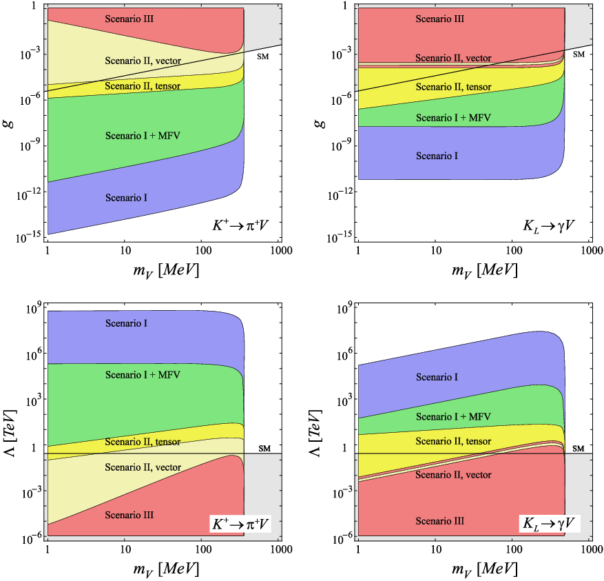
Refer to caption
Figure 4: Above: Exclusion regions drawn from a bound on the K+→π+​VK^{+}\to\pi^{+}V (left) and KL→γ​VK_{L}\to\gamma V (right) branching ratios at the 10−1010^{-10} level. The plots on the first line show the coupling gg as a function of mVm_{V} (in MeV) for the scenario I (blue, g=εVg=\varepsilon_{V}), scenario I with MFV (green, g=εV​|Vt​s∗​Vt​d|g=\varepsilon_{V}|V_{ts}^{\ast}V_{td}|), scenario II from the tensor operators s¯​σμ​ν​d×Vμ​ν\bar{s}\sigma^{\mu\nu}d\times V_{\mu\nu} (yellow) and II from the vector operators s¯​γμ​d×∂νVμ​ν\bar{s}\gamma_{\mu}d\times\partial_{\nu}V^{\mu\nu} (light yellow), and scenario III (g=ε​eg=\varepsilon e). The grey area represents the region where mV/g=vd​a​r​k<v≃246m_{V}/g=v_{dark}<v\simeq 246 GeV. The plots in the second line show the same, but replace gg with Λ=mV/g\Lambda=m_{V}/g (in TeV).
Refer to caption
Figure 5: Constraints on the coupling gg against mVm_{V} from B→K​VB\to KV (left) and B→K∗​VB\to K^{\ast}V (right) for the scenario I (blue, g=ϵVg=\epsilon_{V}), scenario I with MFV (green, g=ϵ​|Vt​b∗​Vt​s|g=\epsilon|V_{tb}^{\ast}V_{ts}|), scenario II from the tensor operators b¯​σμ​ν​s×Vμ​ν\bar{b}\sigma_{\mu\nu}s\times V^{\mu\nu} (yellow) and II from the vector operators b¯​γμ​s×∂νVμ​ν\bar{b}\gamma_{\mu}s\times\partial_{\nu}V^{\mu\nu} (light yellow). The gray areas represent the regions where mV/g=vd​a​r​k<v≃246m_{V}/g=v_{dark}<v\simeq 246 GeV. Lower plots: Same as above, but in terms of Λ=mV/g\Lambda=m_{V}/g (in TeV).

For the operators with two field strengths, we first note that summation over the generators of the adjoint representation of the dark gauge group may be needed to enforce gauge invariance. However, to keep things simple, we consider that after the dark sector symmetry breaking, only one (possibly complex) vector field is light enough to be produced at low energy, and simply discard the adjoint index. In addition, the non-abelian terms of the field strengths are systematically removed since the signatures we are after involve only two vectors. These restrictions, together with 𝒟μ​Vμ​ν=−mV2​Vν\mathcal{D}_{\mu}V^{\mu\nu}=-m_{V}^{2}V^{\nu} and 𝒟μ​V~μ​ν=0\mathcal{D}_{\mu}\tilde{V}^{\mu\nu}=0, permit to reduce all the operators with derivatives acting on the field strengths (as well as those involving Q¯​γμ​(𝒟←ν+𝒟→ν)​Q\bar{Q}\gamma^{\mu}(\overleftarrow{\mathcal{D}}_{\nu}+\overrightarrow{\mathcal{D}}_{\nu})Q). Finally, tensor operators involving two field strengths cannot be constructed since Vμ​ρ​VνρV_{\mu\rho}V_{\,\,\nu}^{\rho} is symmetric under μ↔ν\mu\leftrightarrow\nu, while H†​D¯​σμ​ν​Q×V~μ​ρ​VνρH^{\dagger}\bar{D}\sigma^{\mu\nu}Q\times\tilde{V}_{\mu\rho}V_{\,\,\nu}^{\rho} reduces to H†​D¯​σμ​ν​Q×Vμ​ρ​VνρH^{\dagger}\bar{D}\sigma^{\mu\nu}Q\times V_{\mu\rho}V_{\,\,\nu}^{\rho} upon using 2​σμ​ν​γ5=i​εμ​ν​α​β​σα​β2\sigma^{\mu\nu}\gamma_{5}=i\varepsilon^{\mu\nu\alpha\beta}\sigma_{\alpha\beta}.

Reduction and phenomenology

Not all the operators are relevant phenomenologically. First, we can discard all those involving a derivative acting on the quark fields, since they are comparatively suppressed by 𝒪⁡(mK,B/v)\mathcal{O}(m_{K,B}/v). Then, consider the operators involving ∂μVμ​ν\partial_{\mu}V^{\mu\nu} in ℋm​a​tV[\mathcal{H}_{mat}^{\mathrm{V}}[II]]. Upon enforcing the non-gauge invariant free EOM ∂μVμ​ν=−mV2​Vν\partial_{\mu}V^{\mu\nu}=-m_{V}^{2}V^{\nu}, they collapse to the dimension-four couplings of ℋm​a​tV[\mathcal{H}_{mat}^{\mathrm{V}}[I]], Eq. (28), with the identification

cL,R′VΛ2​(Q¯​γμ​Q,D¯​γμ​D)×∂νVμ​ν→mV2​cL,R′VΛ2​(Q¯​γμ​Q,D¯​γμ​D)×Vμ⇒mV2Λ2​cL,R′V→εL,RV.\frac{c_{L,R}^{\prime V}}{\Lambda^{2}}(\bar{Q}\gamma_{\mu}Q,\bar{D}\gamma_{\mu}D)\times\partial_{\nu}V^{\mu\nu}\to\frac{m_{V}^{2}c_{L,R}^{\prime V}}{\Lambda^{2}}(\bar{Q}\gamma_{\mu}Q,\bar{D}\gamma_{\mu}D)\times V^{\mu}\;\;\Rightarrow\;\frac{m_{V}^{2}}{\Lambda^{2}}c_{L,R}^{\prime V}\to\varepsilon_{L,R}^{V}\;. (36)

This is thus an explicit realization of the ℋm​a​tV[\mathcal{H}_{mat}^{\mathrm{V}}[I]] operators, though with a major difference compared to the previous section. In the mV→0m_{V}\to 0 limit, the coupling εL,RV\varepsilon_{L,R}^{V} here effectively scales at least like mV2m_{V}^{2} instead of mVm_{V}, and the P→P′​VP\to P^{\prime}V rates vanish when mV→0m_{V}\to 0 (compare with Eq. (31)). The precise scaling is not fixed though, because that between cL,R′Vc_{L,R}^{\prime V} and mVm_{V} is not known. If the vector gains its mass at the scale Λ\Lambda from some spontaneous symmetry breaking, all we can say is that mV∼g​Λm_{V}\sim g\Lambda for some gg, and cL,R′V∼gnc_{L,R}^{\prime V}\sim g^{n} for some n≥0n\geq 0, so that εL,RV∼(mV/Λ)2+n\varepsilon_{L,R}^{V}\sim(m_{V}/\Lambda)^{2+n}. This scenario (with n=1n=1, i.e. g=εV=(mV/Λ)3g=\varepsilon_{V}=(m_{V}/\Lambda)^{3}) is shown by the light yellow regions in Figs. 4 and 5. Comparing these regions with those corresponding to the first scenario (in blue), the rescaling (36) is very expensive in terms of accessible scales.

It is interesting to compare the reduction (36) to that of the magnetic operator of ℋm​a​tV[\mathcal{H}_{mat}^{\mathrm{V}}[II]]. After integrating by part and using the quark EOM (21),

cTVΛ2​H†​D¯I​σμ​ν​QJ×Vμ​ν\displaystyle\frac{c_{T}^{V}}{\Lambda^{2}}H^{\dagger}\bar{D}^{I}\mathcal{\sigma}_{\mu\nu}Q^{J}\times V^{\mu\nu} =2​cTVΛ2​H†​H​((Q¯​𝐘d†)I​γμ​QJ+D¯I​γμ​(𝐘d†​D)J)×Vμ\displaystyle=2\frac{c_{T}^{V}}{\Lambda^{2}}H^{\dagger}H((\bar{Q}\mathbf{Y}_{d}^{\dagger})^{I}\gamma_{\mu}Q^{J}+\bar{D}^{I}\gamma_{\mu}(\mathbf{Y}_{d}^{\dagger}D)^{J})\times V^{\mu}
−2icTVΛ2H†D¯I𝒟↔μQJ×Vμ−2cTVΛ2𝒟νH†D¯Iσμ​νQJ×Vμ.\displaystyle\;\;\;\;-2i\frac{c_{T}^{V}}{\Lambda^{2}}H^{\dagger}\bar{D}^{I}\overleftrightarrow{\mathcal{D}}_{\mu}Q^{J}\times V^{\mu}-2\frac{c_{T}^{V}}{\Lambda^{2}}\mathcal{D}^{\nu}H^{\dagger}\bar{D}^{I}\mathcal{\sigma}_{\mu\nu}Q^{J}\times V^{\mu}\;. (37)

The first two terms match those of ℋm​a​tV[\mathcal{H}_{mat}^{\mathrm{V}}[I]], Eq. (28) after electroweak symmetry breaking. Since we started from a gauge-invariant operator, gauge invariance is now hidden in the quark-mass dependent relationships among the couplings εL,RV\varepsilon_{L,R}^{V} of ℋm​a​tV[\mathcal{H}_{mat}^{\mathrm{V}}[I]], as well as of those of the higher-dimensional operators in Eq. (37). It is only upon imposing these relationships that all the terms originating from the kμ​kν/mV2k^{\mu}k^{\nu}/m_{V}^{2} piece of the polarization sum (29) cancel out. Though this is another physically sound interpretation of the ℋm​a​tV[\mathcal{H}_{mat}^{\mathrm{V}}[I]] operators, it is much easier phenomenologically to consider directly the operator H†​D¯I​σμ​ν​QJ×Vμ​νH^{\dagger}\bar{D}^{I}\mathcal{\sigma}_{\mu\nu}Q^{J}\times V^{\mu\nu} of ℋm​a​tV[\mathcal{H}_{mat}^{\mathrm{V}}[II]] from which they derive.

Note, finally, that a similar reduction starting with the last two operators of ℋm​a​tVV[\mathcal{H}_{mat}^{\mathrm{VV}}[II]] can also be done, leading to the leading dimension-six non-gauge invariant operator of Eq. (32)

cS​LV​VΛ4​H†​D¯​Q×Vμ​ν​Vμ​ν∋mV2​cS​LV​VΛ4​H†​D¯​Q×Vν​Vν.\frac{c_{SL}^{VV}}{\Lambda^{4}}H^{\dagger}\bar{D}Q\times V_{\mu\nu}V^{\mu\nu}\ni\frac{m_{V}^{2}c_{SL}^{VV}}{\Lambda^{4}}H^{\dagger}\bar{D}Q\times V_{\nu}V^{\nu}\;. (38)

As explained before, in the present work, we consider this operator exclusively in the gauge invariant form, since the dimension-four couplings of Eq. (28) dominate if no dark gauge invariance is enforced.

After the reductions described above, the only operators relevant for rare FCNC decays are those involving the Higgs field, which we write after the electroweak symmetry breaking as (I>JI>J)

ℋm​a​tV,VV​[II]\displaystyle\mathcal{H}_{mat}^{\mathrm{V},\mathrm{VV}}[\text{II}] =+hS​SI​JΛ3d¯IdJ×Vμ​νVμ​ν+hP​SI​JΛ3d¯Iγ5dJ×Vμ​νVμ​ν+hTI​JΛd¯Iσμ​νdJ×Vμ​ν\displaystyle=+\frac{h_{SS}^{IJ}}{\Lambda^{3}}\bar{d}^{I}d^{J}\times V_{\mu\nu}V^{\mu\nu}+\frac{h_{PS}^{IJ}}{\Lambda^{3}}\bar{d}^{I}\gamma_{5}d^{J}\times V_{\mu\nu}V^{\mu\nu}+\frac{h_{T}^{IJ}}{\Lambda}\bar{d}^{I}\mathcal{\sigma}_{\mu\nu}d^{J}\times V^{\mu\nu}
+i​hS​PI​JΛ3d¯IdJ×Vμ​νV~μ​ν+i​hP​PΛ3d¯Iγ5dJ×Vμ​νV~μ​ν+hT~I​JΛd¯Iσμ​νγ5dJ×Vμ​ν+h.c.,\displaystyle\;\;\;\;+\frac{ih_{SP}^{IJ}}{\Lambda^{3}}\bar{d}^{I}d^{J}\times V_{\mu\nu}\tilde{V}^{\mu\nu}+\frac{ih_{PP}}{\Lambda^{3}}\bar{d}^{I}\gamma_{5}d^{J}\times V_{\mu\nu}\tilde{V}^{\mu\nu}+\frac{h_{\tilde{T}}^{IJ}}{\Lambda}\bar{d}^{I}\mathcal{\sigma}_{\mu\nu}\gamma_{5}d^{J}\times V^{\mu\nu}+h.c.\;\;, (39)

with, omitting flavor indices for simplicity:

hT,T~=vΛ​cT​RV±cT​LV2,hS​S,P​S=vΛ​cS​RV​V±cS​LV​V2,i​hS​P,P​P=vΛ​cS​RV​V~±cS​LV​V~2.h_{T,\tilde{T}}=\frac{v}{\Lambda}\frac{c_{TR}^{V}\pm c_{TL}^{V}}{2},\;h_{SS,PS}=\frac{v}{\Lambda}\frac{c_{SR}^{VV}\pm c_{SL}^{VV}}{2},\;ih_{SP,PP}=\frac{v}{\Lambda}\frac{c_{SR}^{V\tilde{V}}\pm c_{SL}^{V\tilde{V}}}{2}\;. (40)

The rates and differential rates for KK (BB) decays are in Appendix A.5 (B.5), while the physics reach are in Tables 3 to 6. Also, the constraints on the tensor operators are shown by the dark yellow regions in Figs. 4 and 5, setting hT,T~=(v/Λ)​gh_{T,\tilde{T}}=(v/\Lambda)g and Λ=mV/g\Lambda=m_{V}/g.

4.3 Flavor-blind operators

For the last scenario, the invisible vector boson is allowed to couple to conserved quark currents only, so that the singular term in the polarization sum (29) automatically cancels out in decay rate computations. To implement this, we have to drop the S​U​(2)L⊗U​(1)YSU(2)_{L}\otimes U(1)_{Y} gauge invariance requirement (see below), and couple VV to quarks as

ℋe​f​fV​[III]=Jμ​[cq]×Vμ,Jμ​[cq]≡∑q=u,d,s,c,b,tcq​q¯​γμ​q.\mathcal{H}_{eff}^{\mathrm{V}}[\text{III}]=J_{\mu}[c_{q}]\times V^{\mu}\;,\;\;\;\;J_{\mu}[c_{q}]\equiv\sum_{q=u,d,s,c,b,t}c_{q}\bar{q}\gamma_{\mu}q\;. (41)

The cqc_{q} cannot be completely arbitrary but must reflect the flavor structures present in the SM. If that was not the case, then the FCNC couplings (28) of the first scenario are in general present [43], and those would completely dominate in BB and KK decays.

Using the MFV language, there are two possible flavor structures. Either the cqc_{q} are universal or they are proportional to the Yukawa couplings. In the latter case, the top current would completely dominate, corresponding to Class III in the nomenclature of Table 2. In the former case, the remaining freedom corresponds to

cu=cc=ct≡cU,cd=cs=cb≡cD,c_{u}=c_{c}=c_{t}\equiv c_{U}\;,\;\;c_{d}=c_{s}=c_{b}\equiv c_{D}\;, (42)

with cUc_{U} and cDc_{D} a priori arbitrary. Note that this two-parameter freedom means that it is always possible to write Jμ​[cq]J_{\mu}[c_{q}] in terms of the electromagnetic and the baryon number currents only, as was pointed out in Ref. [44]. When the invisible vector is aligned with the photon, rather tight constraints are set by flavor-blind observables, e.g. the muon g−2g-2, quarkonium decays, beam dump experiments (see e.g. Ref. [4] for a recent analysis). While we will compare our constraints with those, let us stress that consistency does not require VμV_{\mu} to couple to leptons77 7 Anomaly cancellation may require the leptons to be charged under the dark gauge symmetry, depending on the detailed particle content and dynamics of the dark sector. We do not consider such constraints.. If it is leptophobic, many of these limits can be evaded. Hence, only the purely hadronic production of VV in KK or BB decays will be considered here, and should be compared e.g. with those from π0\pi^{0} or quarkonium decays with missing energy.

As explained in Sec. 1, it is very different to probe the couplings to heavy (Class III) or to light quarks (Class IV), so we will analyze each situation in turn in the next two sections. But before that, let us return to the issue of an S​U​(2)L⊗U​(1)YSU(2)_{L}\otimes U(1)_{Y} gauge invariant origin for the conserved currents in Eq. (41).

Flavor-blind S​U​(2)L⊗U​(1)YSU(2)_{L}\otimes U(1)_{Y} invariant couplings

In Sec. 4.1, the 1/mV21/m_{V}^{2} singularity of the decay rates arising from the FCNC couplings of Eq. (28) was interpreted in terms of a dark symmetry breaking scale vd​a​r​k≳vv_{dark}\gtrsim v. Specifically, we enforced that the coupling constant ε\varepsilon of VV to quarks and its mass satisfy mV∼vd​a​r​k​εm_{V}\sim v_{dark}\varepsilon, so that it is always the finite combination ε2/mV2→1/vd​a​r​k2\varepsilon^{2}/m_{V}^{2}\to 1/v_{dark}^{2} which occurs in decay rates. But, generic vector or axial-vector quark currents are conserved for massless quarks, which is the case when S​U​(2)L⊗U​(1)YSU(2)_{L}\otimes U(1)_{Y} is exact (for simplicity, we disregard the chiral current anomalies, which do not concern us here). So, the presence of the apparent 1/mV21/m_{V}^{2} singularity could be due to the electroweak symmetry breaking instead of to the dark symmetry breaking.

To make this statement more concrete (see also the discussion in Ref. [46]), let us write down the flavor-blind renormalizable couplings between VV and SM gauge, Higgs, and quark fields (the flavor-blind summation over I=1,2,3I=1,2,3 is understood)

ℋi​n​tV​[III]\displaystyle\mathcal{H}_{int}^{\mathrm{V}}[\text{III}] =ε1​Bμ​ν×Vμ​ν+ε2​i​H†​𝒟↔μ​H×Vμ+εθ​Bμ​ν×V~μ​ν+εH​(H†​H)×Vμ​Vμ,\displaystyle=\varepsilon_{1}B_{\mu\nu}\times V^{\mu\nu}+\varepsilon_{2}iH^{\dagger}\overleftrightarrow{\mathcal{D}}_{\mu}H\times V^{\mu}+\varepsilon_{\theta}B_{\mu\nu}\times\tilde{V}^{\mu\nu}+\varepsilon_{H}(H^{\dagger}H)\times V_{\mu}V^{\mu}\;, (43a)
ℋm​a​tV​[III]\displaystyle\mathcal{H}_{mat}^{\mathrm{V}}[\text{III}] =εB​(Q¯I​γμ​QI+D¯I​γμ​DI+U¯I​γμ​UI)×Vμ+εD​(D¯I​γμ​DI)×Vμ+εU​(U¯I​γμ​UI)×Vμ.\displaystyle=\varepsilon_{B}(\bar{Q}^{I}\gamma_{\mu}Q^{I}+\bar{D}^{I}\gamma_{\mu}D^{I}+\bar{U}^{I}\gamma_{\mu}U^{I})\times V^{\mu}+\varepsilon_{D}(\bar{D}^{I}\gamma_{\mu}D^{I})\times V^{\mu}+\varepsilon_{U}(\bar{U}^{I}\gamma_{\mu}U^{I})\times V^{\mu}\;. (43b)

These dimension-four couplings presumably dominate over the higher dimensional flavor-blind operators, which we do not list here (See Ref. [45]).

Only the ε1\varepsilon_{1}, ε2\varepsilon_{2}, εθ\varepsilon_{\theta}, and εB\varepsilon_{B} couplings are compatible with a dark sector gauge invariance associated to VV, since they vanish under Vμ→∂μϕV^{\mu}\to\partial^{\mu}\phi (see Eq. (31)) upon partial integration, and using the free Higgs boson and quark EOM. The εB\varepsilon_{B} coupling involves the (conserved) baryon number current, and is thus directly matched onto Eq. (41). The other couplings, εH\varepsilon_{H}, εD\varepsilon_{D}, and εU\varepsilon_{U}, would break the dark gauge invariance and are thus discarded. Note that εH\varepsilon_{H} must in any case be tiny if VV is to be light enough to be produced in rare decays. Indeed, the (H†​H)×Vμ​Vμ(H^{\dagger}H)\times V_{\mu}V^{\mu} coupling gives a mass to VV after the electroweak symmetry breaking, so barring a large cancellation between the dark and visible Higgs sectors, εH≲mK⁡(B)2/v2≈10−6​(10−4)\varepsilon_{H}\lesssim m_{K(B)}^{2}/v^{2}\approx 10^{-6}(10^{-4}). We can further discard the εθ\varepsilon_{\theta} term, which is a total derivative and is relevant only for magnetic monopoles [47].

The two remaining couplings are ε1\varepsilon_{1} and ε2\varepsilon_{2}. The first one is the celebrated kinetic mixing [28]. Since Bμ=cos⁡θW​Aμ−sin⁡θW​ZμB_{\mu}=\cos\theta_{W}A_{\mu}-\sin\theta_{W}Z_{\mu}, we can rewrite it as

Bμ​ν×Vμ​ν=2cosθWJνe​m×Vν+2sinθWZν×∂μVμ​ν.B_{\mu\nu}\times V^{\mu\nu}=2\cos\theta_{W}J_{\nu}^{em}\times V^{\nu}+2\sin\theta_{W}Z_{\nu}\times\partial_{\mu}V^{\mu\nu}\;. (44)

The piece proportional to the (conserved) electromagnetic current ∂μFμ​ν=−Jνe​m\partial^{\mu}F_{\mu\nu}=-J_{\nu}^{em} can be matched onto Eq. (41), while the other one mixes ZZ and VV. The ε2\varepsilon_{2} coupling also generates a direct mixing Zμ×VμZ_{\mu}\times V^{\mu} after the electroweak symmetry breaking, since H†​𝒟μ​H→g​v2​ZμH^{\dagger}\mathcal{D}_{\mu}H\to gv^{2}Z_{\mu}.

The Z−VZ-V mixings induced by ε1\varepsilon_{1} and ε2\varepsilon_{2} are very different. The kinetic mixing Zν×∂μVμ​νZ_{\nu}\times\partial_{\mu}V^{\mu\nu} is safe in the mV→0m_{V}\to 0 limit, because it is insensitive to the electroweak symmetry breaking. Actually, once the ZZ is integrated out, this Zν×∂μVμ​νZ_{\nu}\times\partial_{\mu}V^{\mu\nu} vertex together with the SM flavor-changing hadronic vertex of Eq. (30) generate the gauge-invariant operators cL′Vc_{L}^{\prime V} of Eq. (34), with cL′V∼ε1​g3​Vt​I∗​Vt​Jc_{L}^{\prime V}\sim\varepsilon_{1}g^{3}V_{tI}^{\ast}V_{tJ} and Λ∼MZ\Lambda\sim M_{Z}. On the other hand, doing the same with the ε2\varepsilon_{2} coupling generates the dangerous operators of the first scenario, Eq. (28), with

(εLV)I​J∼ε2​g​v2×g2MW2​116​π2​Vt​I∗​Vt​J∼ε2×g16​π2​Vt​I∗​Vt​J.(\varepsilon_{L}^{V})^{IJ}\sim\varepsilon_{2}gv^{2}\times\frac{g^{2}}{M_{W}^{2}}\frac{1}{16\pi^{2}}V_{tI}^{\ast}V_{tJ}\sim\varepsilon_{2}\times\frac{g}{16\pi^{2}}V_{tI}^{\ast}V_{tJ}\;. (45)

However, in parallel to the above FCNC operator, ε2\varepsilon_{2} also corrects the VV mass as δ​mV2∼ε22​v2\delta m_{V}^{2}\sim\varepsilon_{2}^{2}v^{2}. As a result, mVp​h​y​s→0m_{V}^{phys}\to 0 requires ε2→0\varepsilon_{2}\to 0, ensuring again the safety of all decay rates in the massless limit. This shows that indeed, the visible symmetry breaking scale can play the same role as a dark symmetry breaking scale. The only difference, besides v≠vd​a​r​kv\neq v_{dark} in general, is that the former relies on the SM dynamics to drive the FCNC, and thus brings in the loop and CKM suppression factors, see Eq. (45). The allowed range of ε2\varepsilon_{2} values can be derived from the green areas in Figs. 4 and 5, up to the rescaling by g/16​π2∼10−3g/16\pi^{2}\sim 10^{-3}. Note that ε2\varepsilon_{2} values acceptable for rare decays ensure that δ​mV2∼ε22​v2\delta m_{V}^{2}\sim\varepsilon_{2}^{2}v^{2} can be safely neglected.

The above electroweak mechanism ensuring a safe massless limit may render the extension to a two Higgs doublet model desirable. Indeed, there would then be two different εH\varepsilon_{H} couplings, and an additional conserved current can be constructed [37], whose charges are aligned with those of the Peccei-Quinn (PQ) symmetry [48]. Combined with the conserved lepton number current, this allows in principle to make VV completely leptophobic [49]. The cost being the presence of a flavor-blind axial-vector quark current, not conserved at low energy. The corresponding 1/mV21/m_{V}^{2} singularity is nevertheless under control thanks to the additional sources of Z−VZ-V mixing present in the PQ current, i.e. tuned by the same coupling constant. We will not further elaborate on this construction, but just retain that a leptophobic setting is in principle possible, allowing to evade the many low-energy constraints based on the e¯​γμ​e×Vμ\bar{e}\gamma_{\mu}e\times V^{\mu} and μ¯​γμ​μ×Vμ\bar{\mu}\gamma_{\mu}\mu\times V^{\mu} couplings [4, 42].

Apart from the Z−VZ-V mixing effects, matched onto Eq. (28) or Eq. (34), the εB\varepsilon_{B} and ε1\varepsilon_{1} couplings are genuine S​U​(2)L⊗U​(1)YSU(2)_{L}\otimes U(1)_{Y} invariant realization of the two conserved quark currents of Eq. (41). Let us now see how to constrain them from rare decays.

Phenomenological constraints on the couplings to heavy quarks

Once the heavy quarks are integrated out along with the weak bosons, the presence of VV in KK and BB physics is felt through the operators of the second scenario, in particular ℋm​a​tV[\mathcal{H}_{mat}^{\mathrm{V}}[II]]. For example, the last operator in Eq. (34) is induced in complete analogy to the electromagnetic operators describing b→s​γb\to s\gamma and s→d​γs\to d\gamma in the SM. This situation is thus simple to account by adapting the coupling of ℋm​a​tV[\mathcal{H}_{mat}^{\mathrm{V}}[II]] according to Eq. (7), and setting the scale Λ\Lambda at MWM_{W}. Alternatively, a more precise estimate can be obtained when the new invisible vector boson is very light and aligned with the photon (in the quark sector). If we set cU=2/3​ε​ec_{U}=2/3\varepsilon e and cD=−εe/3c_{D}=-\varepsilon e/3, the branching ratios for b→s​Vb\to sV and s→d​Vs\to dV are obtained by rescaling by ε2\varepsilon^{2} the SM predictions for the b→s​γb\to s\gamma and s→d​γs\to d\gamma processes, up to simple phase-space corrections.

Specifically, in the BB sector, the branching ratio for b→s​Vb\to sV is

ℬ⁡(b→s​V)=|ε|2​ℬ​(b→s​γ)SM,ℬ​(b→s​γ)SM=(3.15±0.23)⋅10−4​[50] ,\mathcal{B}(b\to sV)=|\varepsilon|^{2}\mathcal{B}(b\to s\gamma)^{\text{SM}}\;,\;\mathcal{B}(b\to s\gamma)^{\text{SM}}=(3.15\pm 0.23)\cdot 10^{-4}~\text{\cite[cite]{[\@@bibref{}{bsg}{}{}]}\ ,} (46)

when mV≪mBm_{V}\ll m_{B} and Eγ,V>1.6E_{\gamma,V}>1.6 GeV. This cut on the photon energy is actually at the opposite end of phase-space compared to those set for b→s​Xb\to sX. But even without a definite prediction, it is clear that the expected sensitivity of about 10−510^{-5} in the B→(K,K∗)​XB\to(K,K^{\ast})X channels would at best probe ε\varepsilon down to a few percent. For comparison, typical bounds on ε\varepsilon derived from flavor-blind hadronic observables are currently down to the 10−310^{-3} range [4, 42].

The situation is worse in the KK sector, where only CP-violating observables are sensitive to the short-distance (cc and tt) magnetic operator. As analyzed in Ref. [51], those are beyond experimental reach even in the SM case, and thus cannot be used to set constraints on ε\varepsilon. This is actually clear from Table 5: rescaling by ks​d∼10−6k^{sd}\sim 10^{-6}, the scale Λ\Lambda ends up well below the electroweak scale.

So, rare KK and BB decays are rather ineffective at constraining the presence of a new flavor-blind vector coupled exclusively to heavy quarks. Fortunately, in many cases, as e.g. from Eq. (44), universality holds and this vector must also couple to light quarks, where the situation is much better.

Phenomenological constraints on the couplings to light quarks

In this case, the CKM factors strongly favor the KK sector to derive competitive bounds. At the KK mass scale, only the uu, dd, and ss quarks are active quark degrees of freedom. Adopting a matrix notation in the q=(u,d,s)q=(u,d,s) flavor space, ℋe​f​fV[\mathcal{H}_{eff}^{\mathrm{V}}[III]] takes the form

ℋe​f​fV​[III]=e​q¯​γμ​𝐐′​q×Vμ,𝐐′=ε​𝐐+ε′​𝟏,ε≡cU−cDe,ε′≡cU+2​cD3​e,\mathcal{H}_{eff}^{\mathrm{V}}[\text{III}]=e\;\bar{q}\gamma_{\mu}\mathbf{Q}^{\prime}q\times V^{\mu},\;\;\mathbf{Q}^{\prime}=\varepsilon\mathbf{Q}+\varepsilon^{\prime}\mathbf{1}\;,\;\varepsilon\equiv\frac{c_{U}-c_{D}}{e},\;\varepsilon^{\prime}\equiv\frac{c_{U}+2c_{D}}{3e}\;, (47)

with 𝟏=diag(1,1,1)\mathbf{1}=\operatorname*{diag}(1,1,1), 𝐐=diag(2/3,−1/3,−1/3)\mathbf{Q}=\operatorname*{diag}(2/3,-1/3,-1/3), and ee the QED coupling constant. So, from the point of view of low energy physics, there are only two possibilities: either VμV_{\mu} is effectively aligned with the photon (ε\varepsilon term) or its charges are proportional to baryon number (ε′\varepsilon^{\prime} term) [44]. This ℋe​f​fV[\mathcal{H}_{eff}^{\mathrm{V}}[III]] coupling must be directly embedded within Chiral Perturbation Theory (ChPT) [52]. At the leading p2p^{2} order, the VμV^{\mu} field enters only through the covariant derivative acting on the meson fields

Dμ​U=∂μU−i​e​Aμ​[𝐐,U]−i​Vμ​[𝐐′,U]=∂μU−i​e​(Aμ+ε​Vμ)​[𝐐,U].D_{\mu}U=\partial_{\mu}U-ieA_{\mu}\left[\mathbf{Q},U\right]-iV_{\mu}\left[\mathbf{Q}^{\prime},U\right]=\partial_{\mu}U-ie(A_{\mu}+\varepsilon V_{\mu})\left[\mathbf{Q},U\right]\;. (48)

The ε′\varepsilon^{\prime} term cancels out in the commutator, leaving VμV_{\mu} coupled exactly like the photon AμA_{\mu}. This ensures the absence of a direct K→π​VK\to\pi V coupling at leading order, relegating them to 𝒪⁡(p4)\mathcal{O}(p^{4}). Such a direct leading order coupling only exists when the dd and ss charges are different. Indeed, in that case, the generator 𝐐′\mathbf{Q}^{\prime} would no longer commute with that of the weak interaction. This is another way to see that when the universality (42) fails, the dimension-four FCNC couplings of ℋm​a​tV[\mathcal{H}_{mat}^{\mathrm{V}}[I]] should be allowed.

To get bounds on ε\varepsilon is rather immediate since the phenomenology is completely analogous to that of the radiative KK decays (see Ref. [51] for a recent review). It suffices to consider the dominant radiative modes and replace one photon by VV. When it is massless, the rates are obtained from those in QED simply by rescaling by ε2\varepsilon^{2} (or by α′/α\alpha^{\prime}/\alpha, if one defines α′≡ε2​α\alpha^{\prime}\equiv\varepsilon^{2}\alpha). When massive, the amplitudes are essentially the same, the polarization sum is identical (since the QED Ward identity holds), so the main impact is a reduced sensitivity due to the truncated phase-space. Assuming that about 101310^{13} kaon decays will be analyzed in the next generation of experiments, and bounds in the 10−1210^{-12} range are set, the reach in ε\varepsilon is thus naively

ε2≲ℬ⁡(K→n​π+m​γ+V)ℬ⁡(K→n​π+(m+1)​γ)∼10−12ℬ⁡(K→n​π+(m+1)​γ),\varepsilon^{2}\lesssim\frac{\mathcal{B}(K\to n\pi+m\gamma+V)}{\mathcal{B}(K\to n\pi+(m+1)\gamma)}\sim\frac{10^{-12}}{\mathcal{B}(K\to n\pi+(m+1)\gamma)}\;, (49)

for massless (or very light) vector boson VV, and n+m>0n+m>0, n<4n<4. Since the current bounds on ε\varepsilon are down to the 10−310^{-3} range, competitive bounds could be obtained from all the modes with OPENℬ⁡(K→n​π+(m+1)​γ))≳10−7\mathcal{B}(K\to n\pi+(m+1)\gamma))\gtrsim 10^{-7}. Those are listed in Table 7.

Experiment (for V=γV=\gamma) [12] Indicative reach
KL→γ​VK_{L}\to\gamma V 5.47​(4)⋅10−45.47(4)\cdot 10^{-4} |ε,ε′|≲4⋅10−5[mV≪mK]|\varepsilon,\varepsilon^{\prime}|\lesssim 4\cdot 10^{-5}\;[m_{V}\ll m_{K}]
KL→π0​γ​VK_{L}\to\pi^{0}\gamma V 1.273​(34)⋅10−61.273(34)\cdot 10^{-6} |ε|≲1⋅10−3[mV≪mK]|\varepsilon|\lesssim 1\cdot 10^{-3}\;[m_{V}\ll m_{K}]
KS→π0​VK_{S}\to\pi^{0}V −- |ε|≲3⋅10−3[mV≈mπ]|\varepsilon|\lesssim 3\cdot 10^{-3}\;[m_{V}\approx m_{\pi}]
KL→π+​π−​VK_{L}\to\pi^{+}\pi^{-}V 2.83​(11)⋅10−5​[D​E]2.83(11)\cdot 10^{-5}\;[DE] |ε|≲2⋅10−4[mV≪mK]|\varepsilon|\lesssim 2\cdot 10^{-4}\;[m_{V}\ll m_{K}]
K+→π+​γ​VK^{+}\to\pi^{+}\gamma V 1.10​(32)⋅10−61.10(32)\cdot 10^{-6} |ε|≲1⋅10−3[mV≪mK]|\varepsilon|\lesssim 1\cdot 10^{-3}\;[m_{V}\ll m_{K}]
K+→π+​VK^{+}\to\pi^{+}V −- |ε|≲5⋅10−4[mV≈mπ]|\varepsilon|\lesssim 5\cdot 10^{-4}\;[m_{V}\approx m_{\pi}]
K+→π+​π0​VK^{+}\to\pi^{+}\pi^{0}V 6.0​(4)⋅10−6​[D​E]6.0(4)\cdot 10^{-6}\;[DE] |ε|≲4⋅10−4[mV≪mK]|\varepsilon|\lesssim 4\cdot 10^{-4}\;[m_{V}\ll m_{K}]
Table 7: Indicative experimental reach of the radiative decays for a new light vector boson aligned with the photon (ε\varepsilon) or with baryon number (ε′\varepsilon^{\prime}), assuming about 101310^{13} kaon decays are observed and bounds in the 10−1210^{-12} range are set. For the K+→π+​VK^{+}\to\pi^{+}V mode, the reach in |ε||\varepsilon| drops as mVm_{V} decreases (with limits at the 10−310^{-3} level for mV≈50m_{V}\approx 50 MeV, 10−210^{-2} for mV≈5m_{V}\approx 5 MeV, and only 10−110^{-1} for mV≈0.5m_{V}\approx 0.5 MeV).

The K→π​VK\to\pi V channel is special because K→π​γK\to\pi\gamma is forbidden due to gauge invariance. Further, even when off-shell, K→π​γ∗K\to\pi\gamma^{\ast} vanishes at leading order in ChPT, and so does K→π​VK\to\pi V. The leading contribution thus starts at 𝒪⁡(p4)\mathcal{O}(p^{4}), from loops and local counterterms, and is approximately given by [53]

𝒜⁡(K+​(P)→π+​V​(q))=ε​e​GF8​π2​a+​(q2​Pμ−qμ​P⋅q)​εμ∗​(q),\mathcal{A}(K^{+}(P)\to\pi^{+}V(q))=\varepsilon\frac{eG_{F}}{8\pi^{2}}a_{+}\left(q^{2}P^{\mu}-q^{\mu}P\cdot q\right)\varepsilon_{\mu}^{\ast}(q)\;, (50)

with a+a_{+} an 𝒪⁡(1)\mathcal{O}(1) constant. The KSK_{S} rate is expressed similarly in terms of the 𝒪⁡(1)\mathcal{O}(1) constant aSa_{S}, while that for K2≈KLK_{2}\approx K_{L} is CP-violating and thus driven by heavy quarks (since Im⁡(Vu​s∗​Vu​d)=0\operatorname{Im}(V_{us}^{\ast}V_{ud})=0). From this amplitude, we get the rate

Γ⁡(K+→π+​V)=ε2​α​GF2​mK51024​π4​|a+|2​λ3/2​(1,rπ2,rV2)8​π​rV2,\Gamma(K^{+}\to\pi^{+}V)=\varepsilon^{2}\alpha\frac{G_{F}^{2}m_{K}^{5}}{1024\pi^{4}}|a_{+}|^{2}\frac{\lambda^{3/2}(1,r_{\pi}^{2},r_{V}^{2})}{8\pi}r_{V}^{2}\;, (51)

with λ⁡(1,rπ2,rV2)\lambda(1,r_{\pi}^{2},r_{V}^{2}) the kinematical function defined in Eq. (95), and ri=mi/mKr_{i}=m_{i}/m_{K}. Normalizing with the K+→π+​e+​e−K^{+}\to\pi^{+}e^{+}e^{-} process to get rid of a+a_{+},

ℬ⁡(K+→π+​V)=ε2α​3​λ3/2​(1,rπ2,rV2)8​Φe​rV2×ℬ⁡(K+→π+​e+​e−),\mathcal{B}(K^{+}\to\pi^{+}V)=\frac{\varepsilon^{2}}{\alpha}\frac{3\lambda^{3/2}(1,r_{\pi}^{2},r_{V}^{2})}{8\Phi_{e}}r_{V}^{2}\times\mathcal{B}\left(K^{+}\to\pi^{+}e^{+}e^{-}\right)\;, (52)

with Φe≈0.145\Phi_{e}\approx 0.145 the K+→π+​e+​e−K^{+}\to\pi^{+}e^{+}e^{-} phase-space factor, and ℬ⁡(K+→π+​e+​e−)=(3.00±0.09)⋅10−7\mathcal{B}\left(K^{+}\to\pi^{+}e^{+}e^{-}\right)=(3.00\pm 0.09)\cdot 10^{-7} [12]. Reminiscent of K↛π​γK\nrightarrow\pi\gamma, the rate vanishes in the mV→0m_{V}\to 0 limit. This seriously hampers the reach in |ε||\varepsilon|, as indicated in Table 7. Even in the most favorable window mπ≲mV≲2​mπm_{\pi}\lesssim m_{V}\lesssim 2m_{\pi}, K+→π+​VK^{+}\to\pi^{+}V is less sensitive to |ε||\varepsilon| than KL→γ​VK_{L}\to\gamma V by about an order of magnitude, see the red regions in Fig. 4.

To get bounds on ε′\varepsilon^{\prime} is more difficult because it cancels out from the 𝒪⁡(p2)\mathcal{O}(p^{2}) Lagrangian, and thus also from the 𝒪⁡(p4)\mathcal{O}(p^{4}) meson loops (see Eq. (48)). It can thus occur only in some local counterterms involving the Vμ​νV_{\mu\nu} field strength (of vanishing anomalous dimension since there are no divergent loop contributions), and in the odd-parity anomalous 𝒪⁡(p4)\mathcal{O}(p^{4}) Lagrangian. The former are very suppressed compared to the loop contributions induced by QED and by the ε\varepsilon piece, and will be neglected [51].

Concentrating on the odd-parity sector, only the KL→γ​VK_{L}\to\gamma V mode appears useful to constrain ε′\varepsilon^{\prime} (its anomalous amplitude, driven entirely by the up quark [54], is sensitive to both ε\varepsilon and ε′\varepsilon^{\prime}). The magnetic direct emission amplitudes in K→π​π​γK\to\pi\pi\gamma are significantly more suppressed and difficult to access experimentally. Rescaling KL→γ​γK_{L}\to\gamma\gamma according to Eq. (49) shows that a bound on KL→γ​VK_{L}\to\gamma V at the 10−1210^{-12} level would probe couplings down to at least |ε,ε′|≲10−4|\varepsilon,\varepsilon^{\prime}|\lesssim 10^{-4}. Interestingly, this is more than an order of magnitude better than using the flavor-blind transition π0→γ​V\pi^{0}\to\gamma V, for which the best limit is 3.3⋅10−53.3\cdot 10^{-5}, i.e. |ε,ε′|≲6⋅10−3|\varepsilon,\varepsilon^{\prime}|\lesssim 6\cdot 10^{-3} [12]. Further, the range of accessible VV masses is evidently larger in KK decays.

4.4 Baryon and lepton number violating operators

As for the dark scalar, Lorentz invariance requires an even number of SM fermion fields. However, the vector field index allows for alternative chiral structures compared to the Weinberg operators [2]. Specifically, keeping only operators of leading dimensions,

ℋΔ​ℒ=2V,VV\displaystyle\mathcal{H}_{\Delta\mathcal{L}=2}^{\mathrm{V,VV}} =c1IΛ3​H​L¯C​𝒟μ​L​H×Vμ+c2IΛ3​H​L¯C​L​𝒟μ​H×Vμ+c3IΛ3​H​L¯C​L​H×Vμ​Vμ\displaystyle=\frac{c_{1}^{\text{I}}}{\Lambda^{3}}H\bar{L}^{C}\mathcal{D}_{\mu}LH\times V^{\mu}+\frac{c_{2}^{\text{I}}}{\Lambda^{3}}H\bar{L}^{C}L\mathcal{D}_{\mu}H\times V^{\mu}+\frac{c_{3}^{\text{I}}}{\Lambda^{3}}H\bar{L}^{C}LH\times V_{\mu}V^{\mu}
+c1IIΛ3HL¯Cσμ​νLH×Vμ​ν+h.c.,\displaystyle\;\;\;\;+\frac{c_{1}^{\text{II}}}{\Lambda^{3}}H\bar{L}^{C}\sigma_{\mu\nu}LH\times V^{\mu\nu}+h.c.\;, (53a)
ℋΔ​ℬ=−Δ​ℒV,VV\displaystyle\mathcal{H}_{\Delta\mathcal{B}=-\Delta\mathcal{L}}^{\mathrm{V,VV}} =c1,bIΛ3​D¯C​bμ​ν​D×E¯​γν​D×Vμ+c2,bIΛ3​D¯C​bμ​ν​D×L¯​γν​Q×Vμ+h.c.,\displaystyle=\frac{c_{1,b}^{\text{I}}}{\Lambda^{3}}\bar{D}^{C}b_{\mu\nu}D\times\bar{E}\gamma^{\nu}D\times V^{\mu}+\frac{c_{2,b}^{\text{I}}}{\Lambda^{3}}\bar{D}^{C}b_{\mu\nu}D\times\bar{L}\gamma^{\nu}Q\times V^{\mu}+h.c.\;, (53b)
ℋΔ​ℬ=Δ​ℒV,VV\displaystyle\mathcal{H}_{\Delta\mathcal{B}=\Delta\mathcal{L}}^{\mathrm{V,VV}} =c1,aIΛ4​Jaμ×Vμ+c2,aIΛ4​Ja×Vμ​Vμ+c1,aIIΛ4​Jaμ​ν×Vμ​ν+h.c.,\displaystyle=\frac{c_{1,a}^{\text{I}}}{\Lambda^{4}}J_{a}^{\mu}\times V_{\mu}+\frac{c_{2,a}^{\text{I}}}{\Lambda^{4}}J_{a}\times V_{\mu}V^{\mu}+\frac{c_{1,a}^{\text{II}}}{\Lambda^{4}}J_{a}^{\mu\nu}\times V_{\mu\nu}+h.c.\;, (53c)

where the tensor bμ​νb_{\mu\nu} stands for gμ​νg_{\mu\nu} or σμ​ν\sigma_{\mu\nu}, the set a=Q​Q​Q​L,Q​Q​U​E,D​U​U​E,D​U​Q​La=QQQL,QQUE,DUUE,DUQL denotes the gauge-singlet combinations of fields of the Weinberg operators [2], the corresponding currents are defined as

JA​B​C​D\displaystyle J_{ABCD} =A¯C​B×C¯C​D,\displaystyle=\bar{A}^{C}B\times\bar{C}^{C}D\;, (54a)
JA​B​C​Dμ\displaystyle J_{ABCD}^{\mu} =A¯C​𝒟μ​B×C¯C​D,A¯C​B×C¯C​𝒟μ​D,A¯C​𝒟←μ​B×C¯C​D,\displaystyle=\bar{A}^{C}\mathcal{D}^{\mu}B\times\bar{C}^{C}D,\;\bar{A}^{C}B\times\bar{C}^{C}\mathcal{D}^{\mu}D,\;\bar{A}^{C}\overleftarrow{\mathcal{D}}\hskip 0.0pt^{\mu}B\times\bar{C}^{C}D\;, (54b)
JA​B​C​Dμ​ν\displaystyle J_{ABCD}^{\mu\nu} =A¯C​σμ​ν​B×C¯C​D,A¯C​B×C¯C​σμ​ν​D,A¯C​γμ​B×C¯C​γν​D,\displaystyle=\bar{A}^{C}\sigma^{\mu\nu}B\times\bar{C}^{C}D,\;\bar{A}^{C}B\times\bar{C}^{C}\sigma^{\mu\nu}D,\;\bar{A}^{C}\gamma^{\mu}B\times\bar{C}^{C}\gamma^{\nu}D\;, (54c)

and where the S​U​(2)LSU(2)_{L} triplet contraction for the Q​Q​Q​LQQQL current is understood. Note also that c1IIc_{1}^{\text{II}} is antisymmetric in flavor space, c3Ic_{3}^{\text{I}} is symmetric, while c1,2Ic_{1,2}^{\text{I}} have no particular symmetry, though one of them is redundant when flavor-diagonal. For the tensor current, which of the three Dirac structures does exist depends on the chiralities of the fermions involved (and may require reordering the fields using Fierz identities). The only other possible vector current is JDC​U​L​LμJ_{D^{C}ULL}^{\mu}, but it vanishes upon Fierzing due to the antisymmetric S​U​(2)LSU(2)_{L} contraction of the two lepton doublets and thus requires two more Higgs fields. The superscripts I and II refer to the scenarios discussed previously, i.e. separates those operators which explicitly break a dark gauge invariance associated with VV from those which do not.

All these interactions have high dimensions, especially compared to the renormalizable couplings to SM particles of Eqs. (28) and (43). Phenomenologically, they may be relevant only when Λ\Lambda is not too large, which requires the absence of direct FCNC couplings with VV, see Figs. 4 and 5. At the same time, the Δ​ℬ=±Δ​ℒ\Delta\mathcal{B}=\pm\Delta\mathcal{L} interactions can induce nucleon decay when mV<mnm_{V}<m_{n} (note that Δ​ℬ=−Δ​ℒ\Delta\mathcal{B}=-\Delta\mathcal{L} interactions contain at least two dd quarks and do not contribute to p+p^{+} decay at the leading electroweak order), and thus require either the scale Λ\Lambda to be extremely high, or the Wilson coefficients to have highly non-generic flavor structures [11].

A scenario with mB>mV>mnm_{B}>m_{V}>m_{n} is interesting since astrophysical, leptonic, and nucleon decay bounds are essentially circumvented. In that case, rare BB decays into an odd number of baryons (together with an invisible VV) may offer the best windows for the Δ​ℬ=±Δ​ℒ\Delta\mathcal{B}=\pm\Delta\mathcal{L} interactions. Note, though, that if these interactions occur concurrently to those of Eq. (28), (34), or (43), the VV may occur as an intermediate state, bringing back the tight proton decay constraints. It remains to be seen whether in that case, signals in BB decays are nevertheless possible. Such virtual exchanges are beyond our scope, since in the present work, we require the dark particle to be sufficiently long-lived to escape as missing energy in rare decays.

Finally, as for the dark scalar scenario, the Δ​ℒ=2\Delta\mathcal{L}=2 interactions can produce three-body invisible νL​νL​V\nu_{L}\nu_{L}V final states, but are not particularly interesting for FCNC decays. Indeed, they are unable to induce quark flavor transitions, and the FCNC decays would thus proceed through an extremely suppressed hadronic Higgs penguin.

5 Invisible spin-3/2 fermion

Spin-3/23/2 particles are described by Rarita-Schwinger fields, denoted Ψμ\Psi_{\mu}, which transform as spinors with a vector index under the Lorentz group. The corresponding Lagrangian kinetic term can be written as [55]

ℒk​i​n=−12ϵμ​ν​ρ​σΨ¯μγ5γν∂ρΨσ−14mΨΨ¯μ[γμ,γν]Ψν.\mathcal{L}_{kin}=-\frac{1}{2}\epsilon^{\mu\nu\rho\sigma}\overline{\Psi}_{\mu}\gamma_{5}\gamma_{\nu}\partial_{\rho}\Psi_{\sigma}-\frac{1}{4}m_{\Psi}\overline{\Psi}_{\mu}[\gamma^{\mu},\gamma^{\nu}]\Psi_{\nu}\,. (55)

In addition, these fields are also subject to the conditions ​Ψ=0\!\not\!\Psi=0 (spin-3/23/2 projection), (i/∂−mΨ)Ψμ=0(i/\penalty\hskip-5.40608pt\partial-m_{\Psi})\Psi^{\mu}=0 (Dirac equation), and ∂μΨμ=0\partial_{\mu}\Psi^{\mu}=0 (Lorenz condition). For external states, the spin summation is performed as [55]

Π(p)μ​ν=∑s​p​i​nu(p)μsu¯(p)νs=−(/p+mΨ)(Pμ​ν−13Pμ​ρPν​σγργσ),Pα​β≡gα​β−pα​pβmΨ2.\Pi(p)_{\mu\nu}=\sum_{spin}u(p)_{\mu}^{s}\bar{u}(p)_{\nu}^{s}=-(/\penalty\hskip-5.40608ptp+m_{\Psi})(P_{\mu\nu}-\frac{1}{3}P_{\mu\rho}P_{\nu\sigma}\gamma^{\rho}\gamma^{\sigma})\;,\;\;P_{\alpha\beta}\equiv g_{\alpha\beta}-\frac{p_{\alpha}p_{\beta}}{m_{\Psi}^{2}}. (56)

The sum over spin for v​(p)μsv(p)_{\mu}^{s} spinors is given by −Π​(−p)μ​ν-\Pi(-p)_{\mu\nu}.

We distinguish the possible operators for the pair-production of these fields by their Lorenz structures, which can be scalar, vector, or tensor-like (even though Eq. (55) is written down for a Majorana field, Ψ\Psi will be taken as complex from now on). Taking into account the above-stated conditions reduces the possible leading operators to

ℋm​a​tΨ¯​Ψ\displaystyle\mathcal{H}_{mat}^{\overline{\Psi}\Psi} =+cLVΛ2Q¯γμQ×Ψ¯ργμΨρ+cRVΛ2D¯γμD×Ψ¯ργμΨρ+cLAΛ2Q¯γμQ×Ψ¯ργμγ5Ψρ+cRAΛ2D¯γμD×Ψ¯ργμγ5Ψρ\displaystyle=+\frac{c_{L}^{V}}{\Lambda^{2}}\bar{Q}\gamma_{\mu}Q\times\overline{\Psi}^{\rho}\gamma^{\mu}\Psi_{\rho}+\frac{c_{R}^{V}}{\Lambda^{2}}\bar{D}\gamma_{\mu}D\times\overline{\Psi}^{\rho}\gamma^{\mu}\Psi_{\rho}+\frac{c_{L}^{A}}{\Lambda^{2}}\bar{Q}\gamma_{\mu}Q\times\overline{\Psi}^{\rho}\gamma^{\mu}\gamma_{5}\Psi_{\rho}+\frac{c_{R}^{A}}{\Lambda^{2}}\bar{D}\gamma_{\mu}D\times\overline{\Psi}^{\rho}\gamma^{\mu}\gamma_{5}\Psi_{\rho}
+cLSΛ3H†D¯Q×Ψ¯μΨμ+cLPΛ3H†D¯Q×Ψ¯μγ5Ψμ+cRSΛ3HQ¯D×Ψ¯μΨμ+cRPΛ3HQ¯D×Ψ¯μγ5Ψμ\displaystyle\;\;\;\;+\frac{c_{L}^{S}}{\Lambda^{3}}H^{\dagger}\bar{D}Q\times\overline{\Psi}^{\mu}\Psi_{\mu}+\frac{c_{L}^{P}}{\Lambda^{3}}H^{\dagger}\bar{D}Q\times\overline{\Psi}^{\mu}\gamma_{5}\Psi_{\mu}+\frac{c_{R}^{S}}{\Lambda^{3}}H\bar{Q}D\times\overline{\Psi}^{\mu}\Psi_{\mu}+\frac{c_{R}^{P}}{\Lambda^{3}}H\bar{Q}D\times\overline{\Psi}^{\mu}\gamma_{5}\Psi_{\mu}
+cL​STΛ3H†D¯σμ​νQ×Ψ¯[μΨν]+cL​PTΛ3H†D¯σμ​νQ×Ψ¯[μγ5Ψν]+cL​TTΛ3H†D¯σμ​νQ×Ψ¯ρσμ​νΨρ\displaystyle\;\;\;\;+\frac{c_{LS}^{T}}{\Lambda^{3}}H^{\dagger}\bar{D}\sigma_{\mu\nu}Q\times\overline{\Psi}\hskip 0.0pt^{[\mu}\Psi^{\nu]}+\frac{c_{LP}^{T}}{\Lambda^{3}}H^{\dagger}\bar{D}\sigma_{\mu\nu}Q\times\overline{\Psi}\hskip 0.0pt^{[\mu}\gamma_{5}\Psi^{\nu]}+\frac{c_{LT}^{T}}{\Lambda^{3}}H^{\dagger}\bar{D}\sigma_{\mu\nu}Q\times\overline{\Psi}_{\rho}\sigma^{\mu\nu}\Psi^{\rho}
+cR​STΛ3HQ¯σμ​νD×Ψ¯[μΨν]+cR​PTΛ3HQ¯σμ​νD×Ψ¯[μγ5Ψν]+cR​TTΛ3HQ¯σμ​νD×Ψ¯ρσμ​νΨρ,\displaystyle\;\;\;\;+\frac{c_{RS}^{T}}{\Lambda^{3}}H\bar{Q}\sigma_{\mu\nu}D\times\overline{\Psi}\hskip 0.0pt^{[\mu}\Psi^{\nu]}+\frac{c_{RP}^{T}}{\Lambda^{3}}H\bar{Q}\sigma_{\mu\nu}D\times\overline{\Psi}\hskip 0.0pt^{[\mu}\gamma_{5}\Psi^{\nu]}+\frac{c_{RT}^{T}}{\Lambda^{3}}H\bar{Q}\sigma_{\mu\nu}D\times\overline{\Psi}_{\rho}\sigma^{\mu\nu}\Psi^{\rho}\;, (57)

where Ψ¯[μΓΨν]=i(Ψ¯μΓΨν−Ψ¯νΓΨμ)/2\overline{\Psi}\hskip 0.0pt^{[\mu}\Gamma\Psi^{\nu]}=i(\overline{\Psi}\hskip 0.0pt^{\mu}\Gamma\Psi^{\nu}-\overline{\Psi}\hskip 0.0pt^{\nu}\Gamma\Psi^{\mu})/2. Only the leading operators of each kind are kept; operators with additional derivatives are systematically discarded. For the vectorial couplings, the operators involving εμ​ν​ρ​σ​Ψ¯ν​γρ​Ψσ\varepsilon^{\mu\nu\rho\sigma}\overline{\Psi}_{\nu}\gamma_{\rho}\Psi_{\sigma} and εμ​ν​ρ​σ​Ψ¯ν​γ5​γρ​Ψσ\varepsilon^{\mu\nu\rho\sigma}\overline{\Psi}_{\nu}\gamma_{5}\gamma_{\rho}\Psi_{\sigma} have been reduced to the others using the Chisholm identity. Finally, tensor structures are similarly reduced using the Chisholm identity together with σμ​ν​εμ​ν​ρ​σ=−2​i​σρ​σ​γ5\sigma_{\mu\nu}\varepsilon^{\mu\nu\rho\sigma}=-2i\sigma^{\rho\sigma}\gamma_{5}, which in particular permits to get rid of the ϵμ​ν​σ​ρ​Ψ¯σ​γ5​Ψρ\epsilon^{\mu\nu\sigma\rho}\overline{\Psi}_{\sigma}\gamma_{5}\Psi_{\rho} and Ψ¯ρ​σμ​ν​γ5​Ψρ\overline{\Psi}^{\rho}\sigma^{\mu\nu}\gamma_{5}\Psi_{\rho} structures.

The effective couplings of dimensions up to six involving gauge or Higgs fields are easy to construct from those in Eq. (11),

ℋi​n​tΨ¯​Ψ\displaystyle\mathcal{H}_{int}^{\overline{\Psi}\Psi} =+cHSΛH†H×Ψ¯μΨμ+cHPΛH†H×Ψ¯μγ5Ψμ\displaystyle=+\frac{c_{H}^{S}}{\Lambda}H^{\dagger}H\times\overline{\Psi}^{\mu}\Psi_{\mu}+\frac{c_{H}^{P}}{\Lambda}H^{\dagger}H\times\overline{\Psi}^{\mu}\gamma_{5}\Psi_{\mu}
+cBSΛBμ​ν×Ψ¯[μΨν]+cBPΛBμ​ν×Ψ¯[μγ5Ψν]+cBTΛBμ​ν×Ψ¯ρσμ​νΨρ\displaystyle\;\;\;\;+\frac{c_{B}^{S}}{\Lambda}B_{\mu\nu}\times\overline{\Psi}\hskip 0.0pt^{[\mu}\Psi^{\nu]}+\frac{c_{B}^{P}}{\Lambda}B_{\mu\nu}\times\overline{\Psi}\hskip 0.0pt^{[\mu}\gamma_{5}\Psi^{\nu]}+\frac{c_{B}^{T}}{\Lambda}B_{\mu\nu}\times\overline{\Psi}_{\rho}\sigma^{\mu\nu}\Psi^{\rho}
+cB~SΛB~μ​ν×Ψ¯[μΨν]+cB~PΛB~μ​ν×Ψ¯[μγ5Ψν]+cB~TΛB~μ​ν×Ψ¯ρσμ​νΨρ\displaystyle\;\;\;\;+\frac{c_{\tilde{B}}^{S}}{\Lambda}\tilde{B}_{\mu\nu}\times\overline{\Psi}\hskip 0.0pt^{[\mu}\Psi^{\nu]}+\frac{c_{\tilde{B}}^{P}}{\Lambda}\tilde{B}_{\mu\nu}\times\overline{\Psi}\hskip 0.0pt^{[\mu}\gamma_{5}\Psi^{\nu]}+\frac{c_{\tilde{B}}^{T}}{\Lambda}\tilde{B}_{\mu\nu}\times\overline{\Psi}_{\rho}\sigma^{\mu\nu}\Psi^{\rho}
+cHVΛ2iH†𝒟↔μH×Ψ¯ργμΨρ+cHAΛ2iH†𝒟↔μH×Ψ¯ργμγ5Ψρ.\displaystyle\;\;\;\;+\frac{c_{H}^{V}}{\Lambda^{2}}iH^{\dagger}\overleftrightarrow{\mathcal{D}}_{\mu}H\times\overline{\Psi}^{\rho}\gamma^{\mu}\Psi_{\rho}+\frac{c_{H}^{A}}{\Lambda^{2}}iH^{\dagger}\overleftrightarrow{\mathcal{D}}_{\mu}H\times\overline{\Psi}^{\rho}\gamma^{\mu}\gamma_{5}\Psi_{\rho}\;. (58)

After the electroweak symmetry breaking, the situation is similar as for spin 1/2 fields. The dimension-five operators in the first line generate a correction to the Ψ\Psi mass (upon enforcing the ​Ψ=0\!\not\!\Psi=0 constraint), those in the second, third, and fourth line couple Ψ\Psi to the photon and to the ZZ boson. Note, though, that Ψ\Psi does not become millicharged in the usual sense, as these effective operators do not match those derived from the minimal substitution principle (which, in any case, is not consistent for spin 3/2 particles [56]).

The last class is made of operators involving a single Ψ\Psi field. As for the spin-1/2 case, Lorentz invariance requires an odd number of SM fermion fields, so these operators break either baryon or lepton number:

ℋΔ​ℬ,Δ​ℒΨ\displaystyle\mathcal{H}_{\Delta\mathcal{B},\Delta\mathcal{L}}^{\Psi} =c1Δ​ℒΛ𝒟μH×Ψ¯μL+cBΔ​ℒΛ2Bμ​νH×Ψ¯[μγν]L+cWΔ​ℒΛ2Wμ​νiHσi×Ψ¯[μγν]L\displaystyle=\frac{c_{1}^{\Delta\mathcal{L}}}{\Lambda}\mathcal{D}_{\mu}H\times\overline{\Psi}\hskip 0.0pt^{\mu}L+\frac{c_{B}^{\Delta\mathcal{L}}}{\Lambda^{2}}B_{\mu\nu}H\times\overline{\Psi}\hskip 0.0pt^{[\mu}\gamma^{\nu]}L+\frac{c_{W}^{\Delta\mathcal{L}}}{\Lambda^{2}}W_{\mu\nu}^{i}H\sigma^{i}\times\overline{\Psi}\hskip 0.0pt^{[\mu}\gamma^{\nu]}L
+c2Δ​ℒΛ2E¯σμ​νL×Ψ¯[μγν]L+c3Δ​ℒΛ2D¯σμ​νQ×Ψ¯[μγν]L+cΔ​ℬΛ2D¯σμ​νDC×Ψ¯[μγν]UC+h.c..\displaystyle\;\;\;\;+\frac{c_{2}^{\Delta\mathcal{L}}}{\Lambda^{2}}\bar{E}\sigma_{\mu\nu}L\times\overline{\Psi}\hskip 0.0pt^{[\mu}\gamma^{\nu]}L+\frac{c_{3}^{\Delta\mathcal{L}}}{\Lambda^{2}}\bar{D}\sigma_{\mu\nu}Q\times\overline{\Psi}\hskip 0.0pt^{[\mu}\gamma^{\nu]}L+\frac{c^{\Delta\mathcal{B}}}{\Lambda^{2}}\bar{D}\sigma_{\mu\nu}D^{C}\times\overline{\Psi}\hskip 0.0pt^{[\mu}\gamma^{\nu]}U^{C}+h.c.\;. (59)

Notably, compared to the spin-1/2 case (15), no renormalizable coupling can be constructed, and thanks to the extra derivative in the dimension-five operator, there is (of course) no direct mixing between Ψ\Psi and νL\nu_{L} after the electroweak symmetry breaking. Phenomenologically, the signatures for the Δ​ℬ\Delta\mathcal{B} operator would again require specific searches in BB decays, while those for the Δ​ℒ\Delta\mathcal{L} operators are to be found in semileptonic decays. Note, however, that the interactions in Eq. (59) are more difficult to access than those for spin 1/2 invisible particles, Eq. (15), because the tensor matrix elements vanish, ⟨0|d¯I​σμ​ν​uJ|P+⟩=0\langle 0|\bar{d}^{I}\sigma^{\mu\nu}u^{J}|P^{+}\rangle=0. This means that c3Δ​ℒc_{3}^{\Delta\mathcal{L}} does not contribute to the P+→ℓ+​ΨP^{+}\to\ell^{+}\Psi decays, but only enters in the P→P′​ℓ​ΨP\to P^{\prime}\ell\Psi decays for which the helicity-allowed SM contribution P→P′​ℓ​νP\to P^{\prime}\ell\nu is large. Purely leptonic processes are only sensitive to higher-dimensional operators involving covariant derivatives acting on the quark or lepton fields, for example D¯​𝒟μ​Q×Ψ¯μ​L\bar{D}\mathcal{D}_{\mu}Q\times\overline{\Psi}\hskip 0.0pt^{\mu}L. So, the Δ​ℒ\Delta\mathcal{L} operators do not appear promising in searching for dark spin 3/2 particles, and will not be further considered here.

Reduction and phenomenology

The non-conserved quark flavor-changing neutral currents break the gauge symmetry appearing in the Lagrangian (55) when mΨ→0m_{\Psi}\to 0. As a result, the 1/mΨ1/m_{\Psi} terms in the spin sum (56) are not projected out, the massless limit is singular, and we can force Λ\Lambda up to arbitrarily high values simply by decreasing mΨm_{\Psi}. The situation is analogous to that encountered for the massive vector case in Sec. 4.1, and may resolve itself in a fully dynamical theory in a similar way. To get physically meaningful bounds on the scale Λ\Lambda, there are two possible routes.

The first procedure is inspired from the supergravity setting [57], where the spin 3/23/2 gravitino mass is related to the supersymmetry breaking scale as ΛS​U​S​Y=(3​mΨ​MP​l​a​n​c​k)1/2\Lambda_{SUSY}=(\sqrt{3}m_{\Psi}M_{Planck})^{1/2} with MP​l​a​n​c​k=(8πGN)−1/2M_{Planck}=(8\pi G_{N})^{-1/2}. In some sense, this can be understood as the fermionic equivalent of the constraint mV∼g​vd​a​r​km_{V}\sim gv_{dark} enforced for the vector bosons (which would here be insufficient given the harder (mΨ−2)2(m_{\Psi}^{-2})^{2} singularities occurring when there are two spin-3/2 particles in the final state). Indeed, when ΛS​U​S​Y≪MP​l​a​n​c​k\Lambda_{SUSY}\ll M_{Planck}, mΨm_{\Psi}\ is very small and only those terms originating from the mΨ−2m_{\Psi}^{-2} singularity of the spin sum (56) are relevant [55],

Π​(p)μ​ν​=mΨ→0​2​pμ​pν3​mΨ2/p.\Pi(p)_{\mu\nu}\overset{m_{\Psi}\to 0}{=}\frac{2p_{\mu}p_{\nu}}{3m_{\Psi}^{2}}/\penalty\hskip-5.40608ptp\;. (60)

This projects out the ±3/2\pm 3/2 helicity states, leaving the ±1/2\pm 1/2 goldstino helicity states in a way similar to Eq. (31) for the massive vector boson. Specifically, the spin-3/2 operators become equivalent, in the mΨ→0m_{\Psi}\to 0 limit, to the spin-1/2 derivative operators obtained by replacing

Ψμ​=mΨ→0​23​∂μψmΨ.\Psi_{\mu}\overset{m_{\Psi}\to 0}{=}\sqrt{\frac{2}{3}}\frac{\partial_{\mu}\psi}{m_{\Psi}}\,. (61)

Given that the effective operators are at least of dimension six, there are at least two powers of Λ=MP​l​a​n​c​k\Lambda=M_{Planck} which can be eaten away by enforcing Λ​mΨ→ΛS​U​S​Y2\Lambda m_{\Psi}\to\Lambda_{SUSY}^{2}.

The supergravity scenario is thus characterized by the rescaling ΛS​U​S​Y=(3​mΨ​MP​l​a​n​c​k)1/2\Lambda_{SUSY}=(\sqrt{3}m_{\Psi}M_{Planck})^{1/2}. So, even if Ψ\Psi is here not necessarily identified with a light gravitino [58], let us assume that

Λ→Λ¯2/mΨ,\Lambda\to\bar{\Lambda}^{2}/m_{\Psi}\;, (62)

where Λ¯\bar{\Lambda} may not be related to ΛS​U​S​Y\Lambda_{SUSY} in any way but could denote some dark sector symmetry-breaking scale. Phenomenologically, this rescaling permits to derive sensible bounds on Λ¯\bar{\Lambda} from the rare P→P′​Ψ​Ψ¯P\to P^{\prime}\Psi\overline{\Psi} decays, even when mΨ≪mPm_{\Psi}\ll m_{P}.

A second route would start from a basis made entirely of gauge-invariant operators, i.e. involving the field-strength Ψμ​ν≡∂μΨν−∂νΨμ\Psi_{\mu\nu}\equiv\partial_{\mu}\Psi_{\nu}-\partial_{\nu}\Psi_{\mu} and its dual Ψ~μ​ν≡εμ​ν​ρ​σ​∂ρΨσ\tilde{\Psi}_{\mu\nu}\equiv\varepsilon_{\mu\nu\rho\sigma}\partial^{\rho}\Psi^{\sigma}. Though the mΨ→0m_{\Psi}\to 0 limit would always be smooth, we do not perform this construction explicitly because with two field strengths, there are too many operators for the basis to be useful phenomenologically. Instead, we simply remark that starting from such a basis of gauge-invariant operators, it must be possible to generate the ℋm​a​tΨ¯​Ψ\mathcal{H}_{mat}^{\overline{\Psi}\Psi} operators by partial integration and use of the EOM, exactly as for the massive vector boson.

Specifically, when only the spin-3/2 EOM is used, i​γμ​Ψμ​ν=mΨ​Ψνi\gamma_{\mu}\Psi^{\mu\nu}=m_{\Psi}\Psi^{\nu} and γμ​Ψ~μ​ν=−mΨ​γ5​Ψν\gamma_{\mu}\tilde{\Psi}^{\mu\nu}=-m_{\Psi}\gamma_{5}\Psi^{\nu}, an extra factor mΨ2/Λ2m_{\Psi}^{2}/\Lambda^{2} is generated. For example,

1Λ5​H†​D¯​γρ​γν​Q×Ψ¯σ​ρ​γσ​γμ​Ψμ​ν\displaystyle\frac{1}{\Lambda^{5}}H^{\dagger}\bar{D}\gamma^{\rho}\gamma^{\nu}Q\times\overline{\Psi}_{\sigma\rho}\gamma^{\sigma}\gamma^{\mu}\Psi_{\mu\nu} ∼mΨ2Λ5​H†​D¯​γρ​γν​Q×Ψ¯ρ​Ψν,\displaystyle\sim\frac{m_{\Psi}^{2}}{\Lambda^{5}}H^{\dagger}\bar{D}\gamma^{\rho}\gamma^{\nu}Q\times\overline{\Psi}_{\rho}\Psi_{\nu}\;, (63a)
1Λ4​Q¯​γρ​Q×ερ​α​μ​ν​Ψ¯γ​μ​γγ​γα​γβ​Ψβ​ν\displaystyle\frac{1}{\Lambda^{4}}\bar{Q}\gamma_{\rho}Q\times\varepsilon^{\rho\alpha\mu\nu}\overline{\Psi}_{\gamma\mu}\gamma^{\gamma}\gamma^{\alpha}\gamma^{\beta}\Psi_{\beta\nu} ∼mΨ2Λ4​Q¯​γα​Q×Ψ¯μ​γα​Ψμ.\displaystyle\sim\frac{m_{\Psi}^{2}}{\Lambda^{4}}\bar{Q}\gamma_{\alpha}Q\times\overline{\Psi}_{\mu}\gamma^{\alpha}\Psi^{\mu}\;. (63b)

This is analogous to the reduction (36) for the vector boson. By contrast, whenever the reduction involves the quark field EOM (21), the gauge invariance ends up hidden in relationships among the cic_{i} of ℋm​a​tΨ¯​Ψ\mathcal{H}_{mat}^{\overline{\Psi}\Psi}, exactly like in Eq. (37). The resulting operators are then suppressed either by the light quark masses, or by derivatives acting on the quark fields.

Enforcing some cancellations among the operators is incompatible with our procedure of turning on one operator at a time. So, we consider only the situation where the P→P′​Ψ​Ψ¯P\to P^{\prime}\Psi\overline{\Psi} decay rates are finite in the mΨ→0m_{\Psi}\to 0 limit thanks to the rescaling

ci→c¯i​mΨ2Λ2,c_{i}\to\bar{c}_{i}\frac{m_{\Psi}^{2}}{\Lambda^{2}}\;, (64)

with c¯i∼𝒪⁡(1)\bar{c}_{i}\sim\mathcal{O}(1). Note that this cures the singularity (60). Away from the strict mΨ=0m_{\Psi}=0 limit, the other terms of the spin sum (56) also contribute and tend to suppress the rates.

To derive the bounds on the scale Λ\Lambda from the rare decays, we must impose one of the above two prescriptions (62) or (64) to make sense of the mΨ→0m_{\Psi}\to 0 singularities. Comparing them, these rescalings appear precisely equivalent for the dimension-six operators of ℋm​a​tΨ¯​Ψ\mathcal{H}_{mat}^{\overline{\Psi}\Psi}. For the dimension-seven operators, the gravitino-like rescaling (62) leads to an additional suppression by mΨ/Λm_{\Psi}/\Lambda compared to (64), making them completely irrelevant (remember that mΨm_{\Psi} is assumed smaller than mK,Bm_{K,B}). Thus, the bounds we quote for these dimension-seven operators are understood to hold only for the second scenario.

As for the other types of invisible particles, we rewrite the various operators in terms of currents of definite CC and PP by introducing the fourteen complex couplings (for each s→ds\to d, b→sb\to s, and b→db\to d operators)

fX​V,X​A=c¯RX±c¯LX2​(X=V,A),fX​S,X​P=vΛ​c¯RX±c¯LX2​(X=S,P),fT​X,T~​X=vΛ​c¯R​XT±c¯L​XT2​(X=S,P,T).f_{XV,XA}=\frac{\bar{c}_{R}^{X}\pm\bar{c}_{L}^{X}}{2}\;(X=V,A)\;,\;\;f_{XS,XP}=\frac{v}{\Lambda}\frac{\bar{c}_{R}^{X}\pm\bar{c}_{L}^{X}}{2}\;(X=S,P),\;\;f_{TX,\tilde{T}X}=\frac{v}{\Lambda}\frac{\bar{c}_{RX}^{T}\pm\bar{c}_{LX}^{T}}{2}\;(X=S,P,T)\;. (65)

The rates and differential rates are in App. A.6 (B.6) for KK (BB) decays, and the corresponding bounds are shown in Tables 3 and 4. As these numbers show, the rescaling prescription pushes the dimensionality of the operators to eight or nine. For such dimensions, the accessible scales Λ\Lambda are at or even below the electroweak scale, as expected from Eq. (1) and Table 1, and the viability of the S​U​(2)L⊗U​(1)YSU(2)_{L}\otimes U(1)_{Y} effective operator formalism becomes questionable. Said differently, if the scale Λ\Lambda is above the electroweak scale, the presence of a dark spin 3/2 fermion should have no impact on rare FCNC decays.

6 Conclusions

In this paper, we presented a complete basis of S​U​(3)C⊗S​U​(2)L⊗U​(1)YSU(3)_{C}\otimes SU(2)_{L}\otimes U(1)_{Y} invariant operators involving SM fields together with a yet undiscovered light invisible spin 0, 1/2, 1, or 3/2 state, neutral under the SM gauge group. As summarized in Table 8, the operators are organized into three classes: couplings to SM fermions, couplings to SM gauge and/or Higgs fields, and baryon/lepton number violating couplings. We retained the operators of lowest dimensions separately for each class. As a result, most of them do not strictly qualify as portals since they are suppressed by the NP scale Λ\Lambda. However, it makes sense to extend this denomination to those operators for which the experimental constraints push Λ\Lambda far above the electroweak scale. For example, the typical scale for a dimension-five FCNC operator is greater than 10000 TeV (see Table 1), while it can even be close to the Planck scale for those inducing proton decay. For this reason, in the present paper, we systematically investigated the FCNC operators, and derived bounds from the rare FCNC transitions.

ℋm​a​t\mathcal{H}_{mat} Dim ℋi​n​t\mathcal{H}_{int} Dim ℋΔ​ℬ,Δ​ℒ\mathcal{H}_{\Delta\mathcal{B},\Delta\mathcal{L}} Dim
1/2 ψ:ψ​ψ:\begin{array}[c]{r}\psi:\\ \psi\psi:\end{array} −(8)\begin{array}[c]{r}-\\ \text{(\ref{Hspin12})}\end{array} 6\begin{array}[c]{r}\\ 6\end{array} −(11)\begin{array}[c]{r}-\\ \text{(\ref{Spin12Gauge})}\end{array} 5¯\begin{array}[c]{r}\\ \bar{5}\end{array} (15)\begin{array}[c]{r}\text{(\ref{Spin12BL})}\\ \end{array} 6​(4¯)(≥8)\begin{array}[c]{r}6\;(\bar{4})\\ (\geq 8)\end{array}
0 ϕ:ϕ​ϕ:\begin{array}[c]{r}\phi:\\ \phi\phi:\end{array} (20)(23)\begin{array}[c]{r}\text{(\ref{Axion})}\\ \text{(\ref{H2scalars})}\end{array} 5¯6¯\begin{array}[c]{r}\bar{5}\\ \bar{6}\end{array} (25)(26)CLOSE\begin{array}[c]{r}\text{(\ref{HScalarGauge1})}\\ (\text{\ref{HScalarGauge2})}\end{array} 3¯4¯\begin{array}[c]{r}\bar{3}\\ \bar{4}\end{array} (27) 7​(6¯)8​(7¯)\begin{array}[c]{r}7\;(\bar{6})\\ 8\;(\bar{7})\end{array}
1 Direct,Gauge,\begin{array}[c]{r}\text{Direct,}\\ \\ \text{Gauge,}\\ \end{array} V:V​V:V:V​V:\begin{array}[c]{r}V:\\ VV:\\ V:\\ VV:\end{array} (28)(32)(34)(35)\begin{array}[c]{c}\text{(\ref{HvI})}\\ \text{(\ref{HVVI})}\\ \text{(\ref{HvII1})}\\ \text{(\ref{HvII2})}\end{array} 46¯6¯8¯\begin{array}[c]{c}4\\ \bar{6}\\ \bar{6}\\ \bar{8}\end{array} (43) 4¯4¯46¯\begin{array}[c]{c}\bar{4}\\ \bar{4}\\ 4\\ \bar{6}\end{array} (53)(\ref{HVBL}) 7​(7¯)8​(7¯)8​(7¯)10​(9¯)\begin{array}[c]{c}7\;(\bar{7})\\ 8\;(\bar{7})\\ 8\;(\bar{7})\\ 10\;(\bar{9})\end{array}
3/2 Ψ:Ψ​Ψ:\begin{array}[c]{r}\Psi:\\ \Psi\Psi:\end{array} −(57)\begin{array}[c]{r}-\\ \text{(\ref{Hspin3/2})}\end{array} 6\begin{array}[c]{r}\\ 6\end{array} −(58)\begin{array}[c]{r}-\\ (\text{\ref{Hspin32Gauge}})\end{array} 5¯\begin{array}[c]{r}\\ \bar{5}\end{array} (59)\begin{array}[c]{r}\text{(\ref{Spin32BL})}\\ \end{array} 6​(5)(≥8)\begin{array}[c]{r}6\;(5)\\ (\geq 8)\end{array}
Table 8: References in the text for the various pieces of the basis of effective operators. Dimensions are denoted with a bar when the leading operator involves a Higgs field reducible to its vacuum expectation value after the electroweak symmetry breaking. In the last column, the dimensions are indicated for Δ​ℬ\Delta\mathcal{B} operators, irrespective of their Δ​ℒ\Delta\mathcal{L} components, while the dimensions in parenthesis are those of the purely Δ​ℒ\Delta\mathcal{L} operators. For dark vector fields, we distinguish between direct couplings, for which the mV→0m_{V}\to 0 limit is formally divergent, from those where a dark gauge invariance effectively survives (even though full invariance is not imposed, since we allow for mV>0m_{V}>0). Finally, the dimensions of the operators involving spin 3/2 fields increase when ensuring a sensible mΨ→0m_{\Psi}\to 0 limit, see Eqs. (62) and (64).

Our results can be split into two parts: those concerning the basis of operators itself, and those related to its phenomenological impact on the rare decays. Starting with the basis, some of the main features are:

  1. 1.

    First and foremost, it must be stressed that even though we concentrated on the rare KK and BB decays involving missing energy to derive bounds on the operators, our basis is completely general and could be used equally well to investigate signals e.g. in lepton flavor violating transitions, flavor-blind quark or lepton observables, or at high energy colliders (see e.g. Ref. [46]).

  2. 2.

    For all spins, there is in the basis an operator involving only the SM Higgs field coupled to the dark state. Though specific models may not generate such operators, their presence would have two consequences. First, in general, the invisible state can no longer be naturally massless, though it can be very light, since a mass shift arises after the electroweak symmetry breaking. Second, the NP scale should always be greater than the electroweak scale, Λ>v≈246\Lambda>v\approx 246 GeV, otherwise these corrections grow unchecked as powers of H†​HH^{\dagger}H are inserted (this is actually true for all our effective operators). It should be noted though that for spin 1 and spin 3/2 particles, enforcing a dark gauge invariance on the couplings to SM fields explicitly forbids such mass terms.

  3. 3.

    The contribution to FCNC transitions of the flavor-blind operators, i.e. either those involving SM gauge and/or Higgs fields or those involving SM fermion fields of the same flavor, has been clarified. Specifically, for scales Λ\Lambda much higher than the electroweak scale, we pointed out that it is always advantageous to dress flavor-blind operators at the low scale with a WW exchange (see Table 2). Indeed, such a low-scale GIM breaking does not necessitate additional Higgs tadpoles, which would each bring in a 1/Λ1/\Lambda suppression.

  4. 4.

    For spin 1 and 3/2 dark particles, special care was devoted to maintaining a sensible massless limit, or at least to interpret the seemingly divergent limit. Indeed, the flavor-changing neutral currents are not conserved in general, so that the 1/mV21/m_{V}^{2} (1/mΨ21/m_{\Psi}^{2}) term of the polarization (spin) sum is not projected out in physical observables. This is particularly relevant for massive vector states, for which renormalizable couplings to non-conserved quark currents can be constructed. Several mechanisms were discussed, and the corresponding NP scales derived from experimental bounds on the rare decay branching ratios were compared. As shown in Figs. 4 and 5, these scales strongly depend on the assumed dark sector dynamics.

  5. 5.

    All the leading operators producing a single dark fermion, whether of spin 1/2 or 3/2, violate either baryon (ℬ\mathcal{B}) or lepton (ℒ\mathcal{L}) number, but not both simultaneously, and have dimensions smaller or equal to that of the FCNC operators. By contrast, most of the Δ​ℬ\Delta\mathcal{B} and Δ​ℒ\Delta\mathcal{L} violating operators involving a dark vector or scalar particle directly derive from the dimension-six Δ​ℬ=Δ​ℒ=1\Delta\mathcal{B}=\Delta\mathcal{L}=1 Weinberg operators, or from the dimension-five Δ​ℒ=2\Delta\mathcal{L}=2 operator. The former are negligible when they induce proton decay, i.e. when mϕ,V<mpm_{\phi,V}<m_{p}, but could induce exotic BB decays into an odd number of baryons plus missing energy when mB>mϕ,V>mpm_{B}>m_{\phi,V}>m_{p}, since then proton decay is kinematically forbidden. The latter Δ​ℒ=2\Delta\mathcal{L}=2 operators do not induce the quark flavor transitions, hence have a negligible impact on rare decays.

  6. 6.

    To implement the S​U​(2)L⊗U​(1)YSU(2)_{L}\otimes U(1)_{Y} invariance, the FCNC operators are constructed in terms of the SM chiral fermions. Though theoretically sound, and particularly convenient to implement the MFV flavor restrictions, such a basis is not convenient phenomenologically because many of these operators interfere in physical observables. So, our bounds are always derived using the alternative basis of operators obtained by projecting on currents of definite CC and PP. This minimizes interference terms, since in most cases these currents produce different final states.

  7. 7.

    Although many examples of NP models involving new light states were mentioned, no attempt was made to precisely match them onto our basis of operators. Indeed, this would require dwelling into the detailed dynamics and parameters of each model, and would bring us too far from our main objectives, which were to construct the most general basis and constrain its operators from rare FCNC decays.

Concerning the rare FCNC decays of the KK and BB mesons, let us remind that provided the non-standard light states are neutral and sufficiently long-lived, they would show up as missing energy. Those modes cannot be experimentally distinguished from the SM processes producing a neutrino pair in the final state. However, these SM processes are very suppressed, and thus in principle, the rare decays could permit to identify even tiny NP effects. The main outcomes of our detailed phenomenological analysis of such effects are:

  1. 8.

    First, we stressed the importance of including the correct kinematical dependences for probing NP operators. This is crucial because experimentally, the rare decay modes with missing energy do not allow for a complete kinematical reconstruction, and require aggressive background suppressions. In practice, most experimental analyses implicitly assume at various stages that the differential rates have the shapes predicted by the SM, and this seeps through down to the final bounds on the branching ratios. Note, importantly, that these dependences are not always accounted for by simply enforcing the various experimental kinematical cuts. For these reasons, the specific kinematical dependences of each NP effect may have to be implemented by the experimentalists (those are detailed in App. A for KK decays, and App. B for BB decays). This provision has to be kept in mind when interpreting our bounds.

  2. 9.

    In the KK sector, the sensitivities of the KL→XK_{L}\to X, K→π​XK\to\pi X, KL→γ​XK_{L}\to\gamma X, and K→π​π​XK\to\pi\pi X channels were compared, see Tables 3 and 5, with XX a single or a pair of dark particles. The two-body K→XK\to X mode turns out to be the most sensitive, though for a very limited number of operators, but it is also the most difficult to deal with experimentally. At the other extreme, the K→π​π​XK\to\pi\pi X channels are sensitive to nearly all possible operators, but do not appear competitive given their phase-space and chiral suppressions. This leaves the K→π​XK\to\pi X and KL→γ​XK_{L}\to\gamma X channels, whose sensitivities to NP operators are in general comparable. Still, it should be noted that the latter, not yet considered experimentally, has some advantages. First, its SM contribution KL→γ​ν​ν¯K_{L}\to\gamma\nu\bar{\nu} is at the 10−1310^{-13} level (see App. A.3.1), and thus cannot obscure even a tiny NP contribution. Second, for massive flavor-blind dark vector bosons or for millicharged fermions, as derived e.g. from a dark U⁡(1)U(1) kinetically mixed with U​(1)YU(1)_{Y} [28], the KL→γ​XK_{L}\to\gamma X mode is significantly superior to K→π​XK\to\pi X, whose relevant matrix elements vanish at leading order in Chiral Perturbation Theory.

  3. 10.

    In the BB sector, the sensitivities of the Bs,d→XB_{s,d}\to X, B→(K,K∗)​XB\to(K,K^{\ast})X, and B→(π,ρ)​XB\to(\pi,\rho)X decay channels were compared, see Tables 4 and 6. As for KK, the fully invisible decays are both the most sensitive and the most difficult to probe experimentally. The main new feature compared to the KK sector, besides an extended kinematical range allowed for mXm_{X}, is that the modes with two light mesons in the final states can resonate, so that B→K∗​XB\to K^{\ast}X, and B→ρ​XB\to\rho X are competitive. This is particularly interesting since these modes are sensitive to all the quark currents but the scalar b¯​s\bar{b}s and b¯​d\bar{b}d. It should be said also that the present sensitivity of b→sb\to s and b→db\to d decays, in terms of NP scales, is very similar. So, if the NP operators do not follow an MFV-like scaling, a small NP effect could be easier to identify in the latter.

  4. 11.

    The relative sensitivity of KK and BB decays was also compared. As expected, if the flavor structures of the NP operators involving X are generic, KK decays are far more sensitive than BB decays. However, it is well-known that in the visible sector, generic NP flavor structures are at odds with current experimental constraints. If MFV is imposed on both the visible and dark sector operators, the constraints from BB decays become often tighter than from KK decays (see Fig. 3), especially for chirality flipping currents qI​(1,γ5,σμ​ν)​qJq^{I}(1,\gamma_{5},\sigma^{\mu\nu})q^{J}, relatively suppressed by ms/mbm_{s}/m_{b}, and for low-dimensional operators. Indeed, the impact of MFV on the scale Λ\Lambda for an operator of dimension nn decreases as nn increases, since it is approximatively given by ΛM​F​V/Λ≈(Vt​I∗​Vt​J)1/(n−4)\Lambda_{MFV}/\Lambda\approx(V_{tI}^{\ast}V_{tJ})^{1/(n-4)} for the dJ→dId^{J}\to d^{I} transitions, and with the CKM coefficients given in Eq. (6). Note, however, that nn cannot be too large, since rare decay constraints give Λ≲v\Lambda\lesssim v when n≳8n\gtrsim 8, see Table (1). In other words, for Λ≳v\Lambda\gtrsim v, the impact of such operators on the rare decays is beyond reach.

  5. 12.

    The Δ​ℬ\Delta\mathcal{B} and Δ​ℒ\Delta\mathcal{L} operators have low dimensions only for X=ψX=\psi or Ψ\Psi. The Δ​ℬ=1\Delta\mathcal{B}=1 operators can only be probed with specific searches in BB decays involving an odd number of baryons plus missing energy in the final state, and should certainly be included in future experimental programs. For the Δ​ℒ=1\Delta\mathcal{L}=1 effects, the low-dimensional operators are accessible only for X=ψX=\psi, which contribute to P+→ℓ+​ψP^{+}\to\ell^{+}\psi (P=K,D,BP=K,D,B), and would thus apparently enhance the purely leptonic transitions P+→ℓ+​νP^{+}\to\ell^{+}\nu. If the flavor structure of these NP operators is non-universal, this could resolve the persistent discrepancy in B→τ​νB\to\tau\nu while remaining consistent with the B→(e,μ)​νB\to(e,\mu)\nu bounds, as well as, if mψ<mKm_{\psi}<m_{K}, with the tight lepton universality constraint derived from Kℓ​2K_{\ell 2} decays, see Eq. (17).

In conclusion, the presence of a light invisible state weakly coupled to SM particles is not only far from excluded, but is even compelling in many NP models. To find such states, a host of experimental facilities currently available or in planning are called in, from high-intensity meson and lepton factories to high energy colliders, neutrino detectors, earth or space-based direct or indirect dark matter searches, high intensity lasers,… In this big picture, the very rare FCNC decays of the KK and BB mesons, with their unique sensitivities and kinematical ranges, could play a crucial role in the very near future thanks to the leap in luminosity expected at the next generation of experiments, namely NA62 at CERN and K0TO at J-Parc dedicated to these KK decays, and Super-B in Italy and Belle II at KEK aiming for the BB decays.

Acknowledgements

J.F.K. would like to thank Boštjan Golob for sharing his insights regarding experimental acceptances and background suppression in rare decay measurements. This work is supported in part by the Slovenian Research Agency, by the National Science Foundation under Grant No. 1066293 and the hospitality of the Aspen Center for Physics. C. S. would like to thank the J. Stefan Institute, where part of this work was done, for its hospitality.

Appendix A Differential rates for KK decays

A.1 Experimental observables in rare KK decays

Let us start by reviewing the kinematics and current experimental limits for the various KK decays induced by neutral currents and involving missing energy.

A.1.1 K→π+K\to\pi+ missing energy

When the missing energy consists of two invisible particles, the differential rate depends only on the invariant mass of these particles, z≡q2/mK2z\equiv q^{2}/m_{K}^{2}, or equivalently, on the pion momentum Pπ≡|𝐩π|/mK=λ/2P_{\pi}\equiv|\mathbf{p}_{\pi}|/m_{K}=\sqrt{\lambda}/2, with λ≡λ⁡(1,z,rπ2)\lambda\equiv\lambda(1,z,r_{\pi}^{2}) defined in Eq. (95), rπ≡mπ/mKr_{\pi}\equiv m_{\pi}/m_{K}. The phase-space integral is then

ℐπ​X​X=∫4​rX2(1−rπ)2d​z​d​Γd​z​[z]=∫λ1/2​(1,4​rX2,rπ2)/2(1−rπ2)/22​Pπ​d​Pπrπ2+Pπ2​d​Γd​z​[z⁡(Pπ)],\mathcal{I}_{\pi XX}=\int_{4r_{X}^{2}}^{\left(1-r_{\pi}\right)^{2}}dz\,\frac{d\Gamma}{dz}[z]=\int_{\lambda^{1/2}(1,4r_{X}^{2},r_{\pi}^{2})/2}^{(1-r_{\pi}^{2})/2}\frac{2P_{\pi}dP_{\pi}}{\sqrt{r_{\pi}^{2}+P_{\pi}^{2}}}\frac{d\Gamma}{dz}[z(P_{\pi})]\;, (66)

with rX=mX/mKr_{X}=m_{X}/m_{K}.

In the SM, the only available invisible particles are the neutrinos. The SM spectrum for K+→π+​ν​ν¯K^{+}\to\pi^{+}\nu\bar{\nu} and KL→π0​ν​ν¯K_{L}\to\pi^{0}\nu\bar{\nu} then derives entirely from the vector current matrix element ⟨π|s¯​γμ​d|K⟩\langle\pi|\bar{s}\gamma^{\mu}d|K\rangle, and involves the corresponding form-factor (see Eq. (81) in the next Section) slopes λ+′\lambda_{+}^{\prime} and λ+′′\lambda_{+}^{\prime\prime}:

ℐπ​ν​ν¯=∫0(1−rπ)2d​z​λ3/2​|f+K​π​(z)f+K​π​(0)|2=∫0(1−rπ)2d​z​λ3/2​(1+λ+′​zrπ2+λ+′′​z22​rπ4)2,\mathcal{I}_{\pi\nu\bar{\nu}}=\int_{0}^{\left(1-r_{\pi}\right)^{2}}dz\lambda^{3/2}\left|\frac{f_{+}^{K\pi}\left(z\right)}{f_{+}^{K\pi}\left(0\right)}\right|^{2}=\int_{0}^{\left(1-r_{\pi}\right)^{2}}dz\lambda^{3/2}\left(1+\lambda_{+}^{\prime}\frac{z}{r_{\pi}^{2}}+\lambda_{+}^{\prime\prime}\frac{z^{2}}{2r_{\pi}^{4}}\right)^{2}\;\;, (67)

where i=+,0i=+,0. Translated in terms of the pion momentum, i.e. using z⁡(Pπ)=1+rπ2−2​rπ2+Pπ2z(P_{\pi})=1+r_{\pi}^{2}-2\sqrt{r_{\pi}^{2}+P_{\pi}^{2}}, this becomes

ℐπt​o​t=∫0(1−rπ2)/2d​Pπ​16​Pπ4rπ2+Pπ2​(1+λ+′​z⁡(Pπ)rπ2+λ+′′​z​(Pπ)22​rπ4)2.\mathcal{I}_{\pi}^{tot}=\int_{0}^{(1-r_{\pi}^{2})/2}dP_{\pi}\frac{16P_{\pi}^{4}}{\sqrt{r_{\pi}^{2}+P_{\pi}^{2}}}\left(1+\lambda_{+}^{\prime}\frac{z(P_{\pi})}{r_{\pi}^{2}}+\lambda_{+}^{\prime\prime}\frac{z(P_{\pi})^{2}}{2r_{\pi}^{4}}\right)^{2}\;. (68)

The slopes λ+′\lambda_{+}^{\prime} and λ+′′\lambda_{+}^{\prime\prime} are conventionally normalized by the charged pion mass, and are equal for the K+K^{+} and K0K^{0} decays to an excellent approximation (see Ref. [59]). They are extracted from Kℓ​3K_{\ell 3} decays as

λ+′=rλ​(24.82±1.10)⋅10−3,λ+′′=rλ​(1.64±0.44)⋅10−3,rλ=0.990​(5),\lambda_{+}^{\prime}=r_{\lambda}\left(24.82\pm 1.10\right)\cdot 10^{-3}\;,\;\lambda_{+}^{\prime\prime}=r_{\lambda}\left(1.64\pm 0.44\right)\cdot 10^{-3}\;,\;r_{\lambda}=0.990(5)\;, (69)

with rλr_{\lambda} a rescaling factor accounting for the K∗⁣+−K∗0K^{\ast+}-K^{\ast 0} mass difference. These (highly correlated) errors are negligible compared to the experimental and theoretical errors on the integrated rate, and are neglected in Table 9.

Currently, only the charged decay has been observed at Brookhaven [60], in two momentum windows separated by the K+→π+​π0K^{+}\to\pi^{+}\pi^{0} peak, and with the lower end corresponding to the K→π​π​πK\to\pi\pi\pi threshold (see Table 9 and Fig. 6). The proposed charged KK experiment at J-Parc would use the region above the K+→π+​π0K^{+}\to\pi^{+}\pi^{0} peak [61], while the two windows planned at NA62 [62] and proposed at Fermilab [63] are similar. Note that these experiments use very different techniques (stopped vs. in flight), but in both cases, the momentum of the initial and final charged particles are in principle accessible. It is important to stress that not only the combination of the measurements done for each specific window (see Table 9) assumes the SM spectrum, but also that within each window.

For the neutral mode, the KS→π0​ν​ν¯K_{S}\to\pi^{0}\nu\bar{\nu} mode is CP-conserving but difficult to access given the very short KSK_{S} lifetime, so we concentrates on the CP-violating KL→π0​ν​ν¯K_{L}\to\pi^{0}\nu\bar{\nu} mode. The best limit [64]

ℬ⁡(KL→π0​ν​ν¯)<2.6⋅10−8,\mathcal{B}(K_{L}\to\pi^{0}\nu\bar{\nu})<2.6\cdot 10^{-8}\;, (70)

was obtained by the E391a experiment at KEK, and will be further improved using the same techniques at J-Parc [61]. In these experiments, the KLK_{L} momentum is not fixed. So, the high hermeticity of the detector is essential to ensure sufficient suppression of the backgrounds. Though less effective in this case, kinematical cuts are still useful. In particular, the transverse momentum PTP_{T} of the reconstructed π0\pi^{0} is required to be large, between 120120 and 240240 MeV. This does not cut away the background from KL→π0​π0K_{L}\to\pi^{0}\pi^{0}, but rather ensures that the two extra photons have high momentum, and are thus difficult to miss. Since the momentum spectrum of the π0\pi^{0} cannot be directly measured at KEK or J-Parc, and since the SM decay spectrum is implicitly assumed in the analysis, it is far from immediate to translate the current limit (70) into bounds on non-standard currents involving other types of invisible particles.

So, for both the charged and neutral modes, it is not currently possible to deconvolute the SM spectrum from the experimental numbers. To proceed and derive the bounds quoted in the text, we require that the predicted branching ratio for the production of new invisible states does not exceed 10−1010^{-10} when integrated over the momentum windows of the charged mode. This is a rather loose approach, which could significantly underestimate the experimental reach in case the spectrum is very different than the SM one. To illustrate this, note that the bounds for two-body decays are already slightly tighter [65],

ℬ⁡(K+→π+​X0)<0.73⋅10−10​(mX=0).\mathcal{B}(K^{+}\to\pi^{+}X^{0})<0.73\cdot 10^{-10}\;(m_{X}=0)\;. (71)

To improve our naive bounds, either the specific modulations of the spectrum in the presence of NP have to be included throughout the experimental analysis88 8 Brookhaven extracted bounds for purely vector (SM), scalar, or tensor currents, but not for a combination of the SM plus non-standard interactions. Since we cannot turn off the SM rate, this is not directly useful for our purpose., or the true momentum spectrum must be measured (maybe using TOF techniques for the neutral mode [63]). Finally, independently of the NP spectrum, it should be noted that the sensitivity to the K→π​X​(X)K\to\pi X(X) processes is ultimately bounded at around 10−1210^{-12} by the theoretical error on the SM predictions for the K→π​ν​ν¯K\to\pi\nu\bar{\nu} branching ratios.

|pπ|​(M​e​V)|p_{\pi}|\;(MeV) zz ℐπ/ℐπt​o​t\mathcal{I}_{\pi}/\mathcal{I}_{\pi}^{tot} SM Extrapolated total
[ 211, 229][\;211\;,\;229\;] [ 0.000, 0.062][\;0.000\;,\;0.062\;] 27.6%27.6\% 0.228​(18)0.228(18) 1.47−0.89+1.301.47_{-0.89}^{+1.30}
[ 140, 195][\;140\;,\;195\;] [ 0.116, 0.289][\;0.116\;,\;0.289\;] 39.7%39.7\% 0.328​(25)0.328(25) 7.89−5.10+9.267.89_{-5.10}^{+9.26}
Combined (Total BR) – 0.825​(64)0.825(64) 1.73−1.05+1.151.73_{-1.05}^{+1.15}
Table 9: Experimental measurement of K+→π+​ν​ν¯K^{+}\to\pi^{+}\nu\bar{\nu} and SM prediction within each momentum window [60], in units of 10−1010^{-10}.
Refer to caption
Figure 6: The experimental windows in π+\pi^{+} momentum used for controlling backgrounds in the K+→π+​ν​ν¯K^{+}\to\pi^{+}\nu\bar{\nu} measurements, with the seven events seen at Brookhaven. The SM spectrum corresponds to a vector coupling s¯​γμ​d×ν¯L​γμ​νL\bar{s}\gamma_{\mu}d\times\bar{\nu}_{L}\gamma^{\mu}\nu_{L}, and is implicitly implied in computing the branching ratios from the events.

A.1.2 K→π​π+K\to\pi\pi+ missing energy

The phase-space integration for the K→π⁡(K1)​π​(K2)​X​(q)K\to\pi(K_{1})\pi(K_{2})X(q) decays is

ℐπ​π​X=∫4​rπ2(1−rX)2d​y​d​Γd​y,\mathcal{I}_{\pi\pi X}=\int_{4r_{\pi}^{2}}^{(1-r_{X})^{2}}dy\;\frac{d\Gamma}{dy}\;, (72)

with y=(K1+K2)2/mK2y=(K_{1}+K_{2})^{2}/m_{K}^{2} the invariant mass of the pion pair. Compared to K→π​XK\to\pi X, these modes are suppressed by the smaller hadronic matrix elements and by phase-space. Further, the kinematical range is much reduced. Currently, the best limits are (see the respective papers for different mXm_{X} values)

ℬ⁡(K+CLOSE\displaystyle\mathcal{B}(K^{+} →π+π0X0)<4⋅10−5[mX=50MeV][66],\displaystyle\to\pi^{+}\pi^{0}X^{0})<4\cdot 10^{-5}\;[m_{X}=50\;MeV]\;\;\text{\cite[cite]{[\@@bibref{}{PPXE787}{}{}]}}, (73a)
ℬ⁡(KLCLOSE\displaystyle\mathcal{B}(K_{L} →π0π0X0)<7⋅10−7[mX=50MeV][67],\displaystyle\to\pi^{0}\pi^{0}X^{0})<7\cdot 10^{-7}\;[m_{X}=50\;MeV]\;\;\text{\cite[cite]{[\@@bibref{}{PPXE391a}{}{}]}}, (73b)
and are thus very far from Eq. (71). Note that the hadronic matrix elements ⟨π+​π0|s¯​Γ​d|K+⟩\langle\pi^{+}\pi^{0}|\bar{s}\Gamma d|K^{+}\rangle, ⟨π0​π0|s¯​Γ​d|K0⟩\langle\pi^{0}\pi^{0}|\bar{s}\Gamma d|K^{0}\rangle, and ⟨π+​π−|s¯​Γ​d|K0⟩\langle\pi^{+}\pi^{-}|\bar{s}\Gamma d|K^{0}\rangle are related in the isospin limit, see Eq. (94) below, so that these experimental constraints suffice to completely bound the K→π​π​XK\to\pi\pi X system.

The K⁡(P)→π⁡(K1)​π​(K2)​X​(p1)​X¯​(p2)K\left(P\right)\to\pi(K_{1})\pi(K_{2})X(p_{1})\bar{X}(p_{2}) decays are similarly suppressed, and the experimental information is less precise. The phase-space integrals reduce to that over the invariant mass of the invisible pair T2=(p1+p2)2=z​mK2T^{2}=(p_{1}+p_{2})^{2}=zm_{K}^{2} and of the pion pair K2=(K1+K2)2=y​mK2K^{2}=(K_{1}+K_{2})^{2}=ym_{K}^{2}, over the range

ℐπ​π​X​X=∫4​rψ2(1−2​rπ)2d​z​∫4​rπ2(1−z)2d​y​d2​Γd​y​d​z.\mathcal{I}_{\pi\pi XX}=\int_{4r_{\psi}^{2}}^{\left(1-2r_{\pi}\right)^{2}}dz\int_{4r_{\pi}^{2}}^{(1-\sqrt{z})^{2}}dy\;\frac{d^{2}\Gamma}{dydz}\;. (74)

Here again, the SM spectrum critically enters and the current experimental bound

ℬ⁡(K+CLOSE\displaystyle\mathcal{B}(K^{+} OPEN→π+​π0​ν​ν¯)<4.3⋅10−5​[66] ,\displaystyle\to\pi^{+}\pi^{0}\nu\bar{\nu})<4.3\cdot 10^{-5}\;\;\text{\cite[cite]{[\@@bibref{}{PPXE787}{}{}]}\ ,} (75a)
ℬ⁡(KLCLOSE\displaystyle\mathcal{B}(K_{L} OPEN→π0​π0​ν​ν¯)<8.7⋅10−7​[67] ,\displaystyle\to\pi^{0}\pi^{0}\nu\bar{\nu})<8.7\cdot 10^{-7}\;\;\text{\cite[cite]{[\@@bibref{}{PPXE391a}{}{}]}\ ,} (75b)
cannot immediately be translated into bounds for invisible particles of a different type.

Though probably optimistic given the limited phase-space and complicated signatures, we assume bounds of 10−1010^{-10} on each of these K→π​π​XK\to\pi\pi X and K→π​π​X​XK\to\pi\pi XX modes are achievable to derive the numbers in Tables 3 and 5. In any case, if the bounds are different, it is a simple matter to rescale the numbers accordingly. Further, using the same 10−1010^{-10} branching ratio bounds as for the K→π​X​(X)K\to\pi X(X) modes permits to clearly illustrate the reduced sensitivity of the K→π​π​X​(X)K\to\pi\pi X(X) channels.

A.1.3 K→γ+K\to\gamma+ missing energy

Compared to K→π​π​XK\to\pi\pi X and K→π​π​X​XK\to\pi\pi XX, the modes K⁡(P)→γ⁡(k)​X​(p1)​X¯​(p2)K\left(P\right)\to\gamma(k)X(p_{1})\bar{X}(p_{2}) and K⁡(P)→γ⁡(k)​X​(T)K\left(P\right)\to\gamma(k)X(T) are less suppressed and could offer simpler experimental signatures. The phase-space integral for the three-body decay is

ℐγ​X​X=∫4​rX21d​z​d​Γd​z,\mathcal{I}_{\gamma XX}=\int_{4r_{X}^{2}}^{1}dz\;\frac{d\Gamma}{dz}\;, (76)

with z=(p1+p2)2/mK2z=(p_{1}+p_{2})^{2}/m_{K}^{2} the invariant mass of the invisible pair. Despite their theoretical sensitivity, there is currently no experimental limit on these modes. So, for now, we assume that the next generation of experiments will reach ℬ⁡(KL→γ​X)<10−10\mathcal{B}(K_{L}\to\gamma X)<10^{-10}. Note that with about 1012−101310^{12}-10^{13} KLK_{L} decays, as required to measure KL→π0​ν​ν¯K_{L}\to\pi^{0}\nu\bar{\nu}, this may be pessimistic. Further, while the K→π​ν​ν¯K\to\pi\nu\bar{\nu} processes ultimately limits the sensitivity to K→π​X​(X)K\to\pi X(X) at a few 10−1210^{-12} given the current theoretical errors, the SM rate for KL→γ​ν​ν¯K_{L}\to\gamma\nu\bar{\nu} is at the 10−1310^{-13} level, so bounds at or even below that level are in principle achievable.

Other modes with photon and missing energy will not be considered, as the K→n​π+γ+XK\to n\pi+\gamma+X processes are either too suppressed and difficult to access experimentally when fully neutral (given the many photons from the π0\pi^{0}s), or superseded by the non-radiative processes K→n​π+XK\to n\pi+X when some mesons are charged (since the photon of K→n​π+γ+XK\to n\pi+\gamma+X is essentially a bremsstrahlung radiation off the charged meson [68, 69], the amplitude for K→n​π+γ+XK\to n\pi+\gamma+X is actually driven by that for K→n​π+XK\to n\pi+X [70]).

A.1.4 K→K\to missing energy

The simplest decays are those where the KLK_{L} or KSK_{S} simply disappear. Though difficult to probe experimentally, the simpler matrix element together with the minimal number of final state particles strongly enhance their sensitivity to NP effects. In the case of the π0→X​X\pi^{0}\to XX process, the best bound is [71]

ℬ⁡(π0→X​X)<0.27⋅10−6.\mathcal{B}(\pi^{0}\to XX)<0.27\cdot 10^{-6}\;. (77)

But this measurement is actually a by-product of the study of the K+→π+​X​XK^{+}\to\pi^{+}XX decay, since a bound on K+→π+​X​XK^{+}\to\pi^{+}XX indirectly constrains K+→π+π0[→XX]K^{+}\to\pi^{+}\pi^{0}[\to XX]. Doing the same for KL→X​XK_{L}\to XX would require very tight bounds on some BB or DD decays with missing energy, well beyond current capabilities (see Sec. B.1). Alternatively, a direct bound on KL→X​XK_{L}\to XX may be obtained from ϕ\phi factories, where the other KK can be tagged. In deriving NP scales in the text, we will use ℬ⁡(KL→X​X)<10−10\mathcal{B}(K_{L}\to XX)<10^{-10} to simplify the comparison with the other modes, but it should be kept in mind that such a bound appears extremely challenging.

A.2 Matrix elements for KK decays

In the KK sector, the quark currents are represented within Chiral Perturbation Theory (ChPT) [52]. For simplicity, only the leading chiral order is kept. Specifically, the vector and axial-vector currents start at 𝒪⁡(p)\mathcal{O}(p):

q¯LI​γμ​qLJ=i​F22​(Dμ​U†​U)J​I,q¯RI​γμ​qRJ=i​F22​(Dμ​U​U†)J​I,\bar{q}_{L}^{I}\gamma^{\mu}q_{L}^{J}=i\frac{F^{2}}{2}(D^{\mu}U^{\dagger}U)^{JI},\;\;\;\;\bar{q}_{R}^{I}\gamma^{\mu}q_{R}^{J}=i\frac{F^{2}}{2}(D^{\mu}UU^{\dagger})^{JI}\;, (78)

with, at leading order, F=Fπ=92.4F=F_{\pi}=92.4 MeV. Thanks to the QED gauge invariance, there is no unknown low-energy constant in these currents. The scalar and pseudoscalar currents start at 𝒪⁡(p0)\mathcal{O}(p^{0}):

q¯LI​qRJ=−F22​B0​UJ​I,q¯RI​qLJ=−F22​B0​U†J​I,\bar{q}_{L}^{I}q_{R}^{J}=-\frac{F^{2}}{2}B_{0}U^{JI},\;\;\;\bar{q}_{R}^{I}q_{L}^{J}=-\frac{F^{2}}{2}B_{0}U^{\dagger JI}\;\;, (79)

with the low-energy constant B0B_{0} related to the quark masses,

Bs≡B0mK≈(1−rπ2)​mKms=4.6​(8),B_{s}\equiv\frac{B_{0}}{m_{K}}\approx(1-r_{\pi}^{2})\frac{m_{K}}{m_{s}}=4.6(8)\;, (80)

with rπ=mπ/mKr_{\pi}=m_{\pi}/m_{K}, and using ms​(2CLOSEm_{s}(2\,GeVOPEN)=100±20)=100\pm 20 MeV (so when deriving bounds on ci/Λnc_{i}/\Lambda^{n}, ci≡ci​(2CLOSEc_{i}\equiv c_{i}(2\,GeV)) is understood) [12]. The scalar and vector currents are related by the EOM. Specifically, the most general matrix elements for the scalar or vector K→πK\to\pi transitions have the form (z=q2/mK2z=q^{2}/m_{K}^{2}, q=P−Kq=P-K)

⟨π⁡(K)|s¯​d|K⁡(P)⟩∼mK2−mπ2ms−md​f0​(z),⟨π⁡(K)|s¯​γμ​d|K⁡(P)⟩∼(P+K)μ​f+​(z)+(P−K)μ​f−​(z),\langle\pi\left(K\right)|\bar{s}d|K\left(P\right)\rangle\sim\frac{m_{K}^{2}-m_{\pi}^{2}}{m_{s}-m_{d}}f_{0}\left(z\right)\;,\;\langle\pi\left(K\right)|\bar{s}\gamma^{\mu}d|K\left(P\right)\rangle\sim\left(P+K\right)^{\mu}f_{+}\left(z\right)+\left(P-K\right)^{\mu}f_{-}\left(z\right)\;, (81)

up to some simple Clebsch-Gordan coefficient. Taking the divergence of the vector current produces q2​f−​(z)=(mK2−mπ2)​(f0​(z)−f+​(z))q^{2}f_{-}\left(z\right)=(m_{K}^{2}-m_{\pi}^{2})\left(f_{0}\left(z\right)-f_{+}\left(z\right)\right). So, at the leading chiral order, f+,0​(z)=1f_{+,0}\left(z\right)=1 and f−​(z)=0f_{-}\left(z\right)=0. Refinements are only needed for a precise prediction of the SM rates, but are not numerically relevant for the bounds on the production of new invisible states. Note that in practice, the scalar and vector currents do not need to be parametrized as external couplings, but can be directly introduced through the ChPT source terms. Doing this using the leading 𝒪⁡(p2)\mathcal{O}(p^{2}) Lagrangian reproduces Eq. (78) and Eq. (79). We do not consider the next-to-leading 𝒪⁡(p4)\mathcal{O}(p^{4}) meson loops and local terms, except for the odd-parity contact interactions obtained by introducing the vector and axial vector sources in the 𝒪⁡(p4)\mathcal{O}(p^{4}) anomalous Wess-Zumino-Witten (WZW) action [52]. Indeed, owing to their opposite parity, these interactions drive the leading order contributions for some amplitudes.

Finally, from Lorentz and chiral symmetry, combined with parity and charge conjugation (valid for the strong interactions), the most general parametrization for the tensor current starts at 𝒪⁡(p2)\mathcal{O}(p^{2}), where it is given by [51]

q¯I​σμ​ν​PL​qJ\displaystyle\bar{q}^{I}\sigma_{\mu\nu}P_{L}q^{J} =−i​F22​aT​(Dμ​U†​Dν​U​U†−Dν​U†​Dμ​U​U†−i​εμ​ν​ρ​σ​Dρ​U†​Dσ​U​U†)J​I\displaystyle=-i\frac{F^{2}}{2}a_{T}\left(D_{\mu}U^{\dagger}D_{\nu}UU^{\dagger}-D_{\nu}U^{\dagger}D_{\mu}UU^{\dagger}-i\varepsilon_{\mu\nu\rho\sigma}D^{\rho}U^{\dagger}D^{\sigma}UU^{\dagger}\right)^{JI}
+F22​aT′​((Fμ​νL−i​F~μ​νL)​U†+U†​(Fμ​νR−i​F~μ​νR))J​I,\displaystyle\;\;\;\;+\frac{F^{2}}{2}a_{T}^{\prime}((F_{\mu\nu}^{L}-i\tilde{F}_{\mu\nu}^{L})U^{\dagger}+U^{\dagger}(F_{\mu\nu}^{R}-i\tilde{F}_{\mu\nu}^{R}))^{JI}\;\;, (82a)
q¯I​σμ​ν​PR​qJ\displaystyle\bar{q}^{I}\sigma_{\mu\nu}P_{R}q^{J} =−i​F22​aT​(Dμ​U​Dν​U†​U−Dν​U​Dμ​U†​U+i​εμ​ν​ρ​σ​Dρ​U​Dσ​U†​U)J​I\displaystyle=-i\frac{F^{2}}{2}a_{T}\left(D_{\mu}UD_{\nu}U^{\dagger}U-D_{\nu}UD_{\mu}U^{\dagger}U+i\varepsilon_{\mu\nu\rho\sigma}D^{\rho}UD^{\sigma}U^{\dagger}U\right)^{JI}
+F22​aT′​(U⁡(Fμ​νL+i​F~μ​νL)+(Fμ​νR+i​F~μ​νR)​U)J​I.\displaystyle\;\;\;\;+\frac{F^{2}}{2}a_{T}^{\prime}(U(F_{\mu\nu}^{L}+i\tilde{F}_{\mu\nu}^{L})+(F_{\mu\nu}^{R}+i\tilde{F}_{\mu\nu}^{R})U)^{JI}\;. (82b)
Two new low-energy constants aTa_{T} and aT′a_{T}^{\prime} occur, for which we use the Lattice estimates (see the discussion in Ref. [51])
BT​(2​G​e​V)=2​mK​aT=1.21​(12)​ [72],BT′​(2​G​e​V)=2​Fπ​aT′=0.6​(2)​ [73].B_{T}(2\;GeV)=2m_{K}a_{T}=1.21(12)\text{~\cite[cite]{[\@@bibref{}{Mescia00}{}{}]}}\;,\;\;B_{T}^{\prime}(2\;GeV)=2F_{\pi}a_{T}^{\prime}=0.6(2)\text{~\cite[cite]{[\@@bibref{}{MS}{}{}]}}\;. (83)

Note that a more recent lattice estimate BT=0.65​(2)B_{T}=0.65(2) [74] is two times smaller, and thus suppresses the sensitivity of KK decays to the tensor currents. Still, in terms of the NP scales Λ\Lambda given in the Tables 3 and 5, the precise value of BTB_{T} is not that relevant at present since these numbers are to be understood as order of magnitude estimates.

So, altogether, and defining Γ≡cS+cP​γ5+cV​γμ+cA​γμ​γ5+cT​σμ​ν+cT~​σμ​ν​γ5\Gamma\equiv c_{S}+c_{P}\gamma_{5}+c_{V}\gamma^{\mu}+c_{A}\gamma^{\mu}\gamma_{5}+c_{T}\sigma_{\mu\nu}+c_{\tilde{T}}\sigma_{\mu\nu}\gamma_{5}, the matrix elements in the isospin limit and to the leading chiral order are99 9 A number of sign conventions are implicitly defined by these equations. We closely follow the ChPT conventions of [52, 51]

2​⟨0​|s¯​Γ​d|​K0​(P)⟩\displaystyle\sqrt{2}\langle 0|\bar{s}\Gamma d|K^{0}(P)\rangle =2​i​Fπ​(−B0​cP+Pμ​cA),\displaystyle=2iF_{\pi}\left(-B_{0}c_{P}+P^{\mu}c_{A}\right)\;, (84a)
2​⟨γ⁡(k,α)​|s¯​Γ​d|​K0​(P)⟩\displaystyle\sqrt{2}\langle\gamma(k,\alpha)|\bar{s}\Gamma d|K^{0}(P)\rangle =−43​e​Fπ​(aT′​cT~​(kμ​gα​ν−kν​gα​μ)−i​aT′​cT​ϵα​μ​ν​ρ​kρ+cV​NC8​π2​Fπ2​εα​μ​ρ​σ​kρ​Pσ),\displaystyle=-\frac{4}{3}eF_{\pi}(a_{T}^{\prime}c_{\tilde{T}}\left(k^{\mu}g^{\alpha\nu}-k^{\nu}g^{\alpha\mu}\right)-ia_{T}^{\prime}c_{T}\epsilon^{\alpha\mu\nu\rho}k_{\rho}+\frac{c_{V}N_{C}}{8\pi^{2}F_{\pi}^{2}}\varepsilon^{\alpha\mu\rho\sigma}k_{\rho}P_{\sigma})\;\;, (84b)
2​⟨π0​(K)|s¯​Γ​d|K0​(P)⟩\displaystyle\sqrt{2}\langle\pi^{0}(K)|\bar{s}\Gamma d|K^{0}(P)\rangle =−⟨π+​(K)|s¯​Γ​d|K+​(P)⟩\displaystyle=-\langle\pi^{+}(K)|\bar{s}\Gamma d|K^{+}(P)\rangle
=−B0cS+(Pμ+Kμ)cV+2aT(icTK[μPν]−cT~εμ​ν​ρ​σKρPσ),\displaystyle=-B_{0}c_{S}+(P^{\mu}+K^{\mu})c_{V}+2a_{T}\left(ic_{T}K^{[\mu}P^{\nu]}-c_{\tilde{T}}\varepsilon^{\mu\nu\rho\sigma}K_{\rho}P_{\sigma}\right)\;\;, (84c)
and
−⟨π+​(K1)​π0​(K2)|s¯​Γ​d|K+​(P)⟩=ℳ−​(K→π​π),2​⟨π0​(K1)​π0​(K2)|s¯​Γ​d|K0​(P)⟩=ℳ+​(K→π​π),\displaystyle-\langle\pi^{+}(K_{1})\pi^{0}(K_{2})|\bar{s}\Gamma d|K^{+}(P)\rangle=\mathcal{M}_{-}\left(K\to\pi\pi\right),\;\sqrt{2}\langle\pi^{0}(K_{1})\pi^{0}(K_{2})|\bar{s}\Gamma d|K^{0}(P)\rangle=\mathcal{M}_{+}\left(K\to\pi\pi\right)\;\;,
2​⟨π+​(K1)​π−​(K2)|s¯​Γ​d|K0​(P)⟩=ℳ+​(K→π​π)+ℳ−​(K→π​π),\displaystyle\sqrt{2}\langle\pi^{+}(K_{1})\pi^{-}(K_{2})|\bar{s}\Gamma d|K^{0}(P)\rangle=\mathcal{M}_{+}\left(K\to\pi\pi\right)+\mathcal{M}_{-}\left(K\to\pi\pi\right)\;\;, (85a)
with
ℳ+​(K→π​π)\displaystyle\mathcal{M}_{+}(K\to\pi\pi) =i​B0​cPFπK+⋅T−mK2−T−2−i​cAFπ(K+μ+T−μ​K+⋅T−mK2−T−2)+aTFπ(cT~K+[μT−ν]−icTεμ​ν​ρ​σT−ρK+σ),\displaystyle=\frac{iB_{0}c_{P}}{F_{\pi}}\frac{K_{+}\cdot T_{-}}{m_{K}^{2}-T_{-}^{2}}-\frac{ic_{A}}{F_{\pi}}\left(K_{+}^{\mu}+\frac{T_{-}^{\mu}K_{+}\cdot T_{-}}{m_{K}^{2}-T_{-}^{2}}\right)+\frac{a_{T}}{F_{\pi}}\left(c_{\tilde{T}}K_{+}^{[\mu}T_{-}^{\nu]}-ic_{T}\varepsilon^{\mu\nu\rho\sigma}T_{-\rho}K_{+\sigma}\right), (86a)
ℳ−​(K→π​π)\displaystyle\mathcal{M}_{-}(K\to\pi\pi) =−i​B0​cPFπK−⋅T−mK2−T−2+i​cAFπ(K−μ+T−μ​K−⋅T−mK2−T−2)+aTFπ(cT~K−[νT+μ]+icTεμ​ν​ρ​σT+ρK−σ)\displaystyle=-\frac{iB_{0}c_{P}}{F_{\pi}}\frac{K_{-}\cdot T_{-}}{m_{K}^{2}-T_{-}^{2}}+\frac{ic_{A}}{F_{\pi}}\left(K_{-}^{\mu}+\frac{T_{-}^{\mu}K_{-}\cdot T_{-}}{m_{K}^{2}-T_{-}^{2}}\right)+\frac{a_{T}}{F_{\pi}}\left(c_{\tilde{T}}K_{-}^{[\nu}T_{+}^{\mu]}+ic_{T}\varepsilon^{\mu\nu\rho\sigma}T_{+\rho}K_{-\sigma}\right)
−cV​NC​εμ​ν​ρ​σ​K+ν​K−ρ​T−σ12​π2​Fπ3,\displaystyle\;\;\;\;-\frac{c_{V}N_{C}\varepsilon^{\mu\nu\rho\sigma}K_{+\nu}K_{-\rho}T_{-\sigma}}{12\pi^{2}F_{\pi}^{3}}\;, (86b)
where K±=K2±K1K_{\pm}=K_{2}\pm K_{1}, T±=P±K+T_{\pm}=P\pm K_{+}, and X[μYν]=XμYν−XνYμX^{[\mu}Y^{\nu]}=X^{\mu}Y^{\nu}-X^{\nu}Y^{\mu}. Terms proportional to the number of QCD colors, NC=3N_{C}=3, come from the WZW action. The mK2−T−2m_{K}^{2}-T_{-}^{2} denominators arise from the kaon pole topologies, K→π​π​K0K\to\pi\pi K^{0} followed by K0→0K^{0}\to 0 (from Eq. (84)). Note that ℳ+​(K→π​π)\mathcal{M}_{+}(K\to\pi\pi) is even under K1↔K2K_{1}\leftrightarrow K_{2}, while ℳ−​(K→π​π)\mathcal{M}_{-}(K\to\pi\pi) is odd, hence these amplitudes describe two-pion states with even and odd orbital angular momentum, respectively. The π0​π0\pi^{0}\pi^{0} state is purely even due to Bose statistics, while the π+​π0\pi^{+}\pi^{0} state has total isospin one, hence is purely odd.

Only the tensor currents contribute to the ℳ⁡(K→γ)\mathcal{M}(K\to\gamma) amplitude at tree-level. So, it may seem that together with the 𝒪⁡(p4)\mathcal{O}(p^{4}) WZW amplitude, we should include also the even-parity meson loops along with their counterterms. However, for neutral current sources, i.e., in terms of Gell-Mann matrices, for vμ,aμ,s,p∼λ6±i​λ7v_{\mu},a_{\mu},s,p\sim\lambda_{6}\pm i\lambda_{7}, the only allowed even-parity K→γK\to\gamma matrix elements vanish when the photon is on-shell

⟨γ⁡(q,ν)​|s¯​γ5​d|​K0​(P)⟩\displaystyle\langle\gamma(q,\nu)|\bar{s}\gamma_{5}d|K^{0}(P)\rangle =i​e​B072​2​π2​Fπ​q2​Tν−qν​q⋅TT2−mK2​Φ⁡(q2,mK2)−Φ⁡(q2,mπ2)q2,\displaystyle=\frac{ieB_{0}}{72\sqrt{2}\pi^{2}F_{\pi}}\frac{q^{2}T^{\nu}-q^{\nu}q\cdot T}{T^{2}-m_{K}^{2}}\frac{\Phi(q^{2},m_{K}^{2})-\Phi(q^{2},m_{\pi}^{2})}{q^{2}}\;, (87a)
⟨γ⁡(q,ν)​|s¯​γμ​γ5​d|​K0​(P)⟩\displaystyle\langle\gamma(q,\nu)|\bar{s}\gamma^{\mu}\gamma_{5}d|K^{0}(P)\rangle =i​e72​2​π2​Fπ​[qμ​qν−q2​gμ​ν+Tμ​q2​Tν−qν​q⋅TT2−mK2]​Φ⁡(q2,mK2)−Φ⁡(q2,mπ2)q2,\displaystyle=\frac{ie}{72\sqrt{2}\pi^{2}F_{\pi}}\left[q^{\mu}q^{\nu}-q^{2}g^{\mu\nu}+T^{\mu}\frac{q^{2}T^{\nu}-q^{\nu}q\cdot T}{T^{2}-m_{K}^{2}}\right]\frac{\Phi(q^{2},m_{K}^{2})-\Phi(q^{2},m_{\pi}^{2})}{q^{2}}\;, (87b)
where T=P−qT=P-q, and Φ⁡(q2,m2)\Phi(q^{2},m^{2}) the loop functions occurring for K→π​γ∗K\to\pi\gamma^{\ast} (see e.g. Ref. [68]), defined in terms of the standard scalar one-loop integrals as
Φ⁡(q2,m2)=3​(q2−4​m2)​B0​(q2,m2,m2)+12​m2​B0​(0,m2,m2)−2​q2.\Phi(q^{2},m^{2})=3(q^{2}-4m^{2})B_{0}(q^{2},m^{2},m^{2})+12m^{2}B_{0}(0,m^{2},m^{2})-2q^{2}\;. (88)

Contrary to K→π​γ∗K\to\pi\gamma^{\ast}, the FCNC matrix elements are finite since the UV divergences cancel in the difference between the K±K^{\pm} and π±\pi^{\pm} loop contributions, and there are no counterterms. Though in principle, the K→ℓ+​ℓ−​XK\to\ell^{+}\ell^{-}X modes could thus offer precise probes, their rates are far too suppressed by α\alpha, the loop factors, and the cancellation between the K±K^{\pm} and π±\pi^{\pm} loops. So, only K→γ​XK\to\gamma X will be considered here, which is thus induced exclusively by tensor currents and 𝒪⁡(p4)\mathcal{O}(p^{4}) anomalous interactions.

Finally, the operator basis also includes vector and scalar currents with a covariant derivative. Though these operators are never retained in deriving bounds on the new physics scale in the main text, for the sake of completeness, let us nevertheless write down the relevant chiral realizations. For the vector currents, extending the analysis of Ref. [75], we write

q¯I​D←α​γμ​PL​qJ\displaystyle\bar{q}^{I}\overleftarrow{D}_{\alpha}\gamma_{\mu}P_{L}q^{J} =i​F24​(∂μU†​∂αU+∂α∂μU†​U−18​gα​μ​(χ†​U+U†​χ)+aV​i​εα​μ​β​ν​∂βU†​∂νU)J​I,\displaystyle=i\frac{F^{2}}{4}(\partial_{\mu}U^{\dagger}\partial_{\alpha}U+\partial_{\alpha}\partial_{\mu}U^{\dagger}U-\frac{1}{8}g_{\alpha\mu}(\chi^{\dagger}U+U^{\dagger}\chi)+a_{V}i\varepsilon_{\alpha\mu\beta\nu}\partial^{\beta}U^{\dagger}\partial^{\nu}U)^{JI}\;, (89a)
q¯I​D←α​γμ​PR​qJ\displaystyle\bar{q}^{I}\overleftarrow{D}_{\alpha}\gamma_{\mu}P_{R}q^{J} =i​F24​(∂μU​∂αU†+∂α∂μU​U†−18​gα​μ​(χ​U†+U​χ†)−aV​i​εα​μ​β​ν​∂βU​∂νU†)J​I,\displaystyle=i\frac{F^{2}}{4}(\partial_{\mu}U\partial_{\alpha}U^{\dagger}+\partial_{\alpha}\partial_{\mu}UU^{\dagger}-\frac{1}{8}g_{\alpha\mu}(\chi U^{\dagger}+U\chi^{\dagger})-a_{V}i\varepsilon_{\alpha\mu\beta\nu}\partial^{\beta}U\partial^{\nu}U^{\dagger})^{JI}\;, (89b)
q¯I​γμ​PL​D→α​qJ\displaystyle\bar{q}^{I}\gamma^{\mu}P_{L}\overrightarrow{D}_{\alpha}q^{J} =−i​F24​(∂αU†​∂μU+U†​∂α∂μU−18​gα​μ​(U†​χ+χ†​U)+aV​i​εα​μ​β​ν​∂βU†​∂νU)J​I,\displaystyle=-i\frac{F^{2}}{4}(\partial_{\alpha}U^{\dagger}\partial_{\mu}U+U^{\dagger}\partial_{\alpha}\partial_{\mu}U-\frac{1}{8}g_{\alpha\mu}(U^{\dagger}\chi+\chi^{\dagger}U)+a_{V}i\varepsilon_{\alpha\mu\beta\nu}\partial^{\beta}U^{\dagger}\partial^{\nu}U)^{JI}\;, (89c)
q¯I​γμ​PR​D→α​qJ\displaystyle\bar{q}^{I}\gamma_{\mu}P_{R}\overrightarrow{D}_{\alpha}q^{J} =−i​F24​(∂αU​∂μU†+U​∂α∂μU†−18​gα​μ​(U​χ†+χ​U†)−aV​i​εα​μ​β​ν​∂βU​∂νU†)J​I.\displaystyle=-i\frac{F^{2}}{4}(\partial_{\alpha}U\partial_{\mu}U^{\dagger}+U\partial_{\alpha}\partial_{\mu}U^{\dagger}-\frac{1}{8}g_{\alpha\mu}(U\chi^{\dagger}+\chi U^{\dagger})-a_{V}i\varepsilon_{\alpha\mu\beta\nu}\partial^{\beta}U\partial^{\nu}U^{\dagger})^{JI}\;. (89d)
Most of the terms are fixed by taking divergences and imposing the EOM, but for the constant aVa_{V}, a priori of 𝒪⁡(1)\mathcal{O}(1). For the scalar currents, the chiral realizations start at 𝒪⁡(p)\mathcal{O}(p),
q¯I​PR​D→α​qJ\displaystyle\bar{q}^{I}P_{R}\overrightarrow{D}_{\alpha}q^{J} =q¯I​PR​D←α​qJ=−F24​B0​(Dα​U)J​I,\displaystyle=\bar{q}^{I}P_{R}\overleftarrow{D}_{\alpha}q^{J}=-\frac{F^{2}}{4}B_{0}(D_{\alpha}U)^{JI}, (90a)
q¯I​PL​D→α​qJ\displaystyle\bar{q}^{I}P_{L}\overrightarrow{D}_{\alpha}q^{J} =q¯I​PL​D←α​qJ=−F24​B0​(Dα​U†)J​I.\displaystyle=\bar{q}^{I}P_{L}\overleftarrow{D}_{\alpha}q^{J}=-\frac{F^{2}}{4}B_{0}(D_{\alpha}U^{\dagger})^{JI}\;. (90b)
These currents are completely fixed by imposing parity and charge conjugation, together with
q¯J​PL,R​D→α​qI+q¯J​D←α​PL,R​qI=∂α(q¯J​PL,R​qI).\bar{q}^{J}P_{L,R}\overrightarrow{D}_{\alpha}q^{I}+\bar{q}^{J}\overleftarrow{D}_{\alpha}P_{L,R}q^{I}=\partial_{\alpha}(\bar{q}^{J}P_{L,R}q^{I})\;. (91)

Note, however, that the above chiral representations lead to q¯I​(D→α−D←α)​PL,R​qJ=0\bar{q}^{I}(\overrightarrow{D}_{\alpha}-\overleftarrow{D}_{\alpha})P_{L,R}q^{J}=0 instead of (mI2−mJ2)​q¯I​PL,R​qJ(m_{I}^{2}-m_{J}^{2})\bar{q}^{I}P_{L,R}q^{J}. This is because while q¯I​(D→α+D←α)​PL,R​qJ\bar{q}^{I}(\overrightarrow{D}_{\alpha}+\overleftarrow{D}_{\alpha})P_{L,R}q^{J} is of 𝒪⁡(p)\mathcal{O}(p), the difference q¯I​(D→α−D←α)​PL,R​qJ\bar{q}^{I}(\overrightarrow{D}_{\alpha}-\overleftarrow{D}_{\alpha})P_{L,R}q^{J} is actually of 𝒪⁡(p3)\mathcal{O}(p^{3}) since quark masses are 𝒪⁡(p2)\mathcal{O}(p^{2}). So, terms at that order would be required to get a correct divergence.

A.2.1 Decay rates in the isospin limit

The strong matrix elements (84–86) are derived in the isospin limit. As a result, all the differential decay rates can be reconstructed entirely from those of the KL≈K2K_{L}\approx K_{2}. The contributions coming from the ε​K1\varepsilon K_{1} piece of the KLK_{L}, suppressed by ε∼2⋅10−3\varepsilon\sim 2\cdot 10^{-3}, are neglected here.

For the K→(γ)​XK\to(\gamma)X modes, the KS≈K1K_{S}\approx K_{1} rates are obtained from those for KL≈K2K_{L}\approx K_{2} by interchanging the real and imaginary parts of the couplings x=fix=f_{i}, gig_{i}, hih_{i}:

d​Γ​(KS→(γ)​X)d​z=d​Γ​(KL→(γ)​X)d​z[ℑ(x)↔ℜ(x)].\frac{d\Gamma\left(K_{S}\to(\gamma)X\right)}{dz}=\frac{d\Gamma\left(K_{L}\to(\gamma)X\right)}{dz}\left[\Im(x)\leftrightarrow\Re(x)\right]\;. (92)

The K+→π+​XK^{+}\to\pi^{+}X decay rates are proportional to the sum Γ⁡(KS→π0​X)+Γ⁡(KL→π0​X)\Gamma(K_{S}\to\pi^{0}X)+\Gamma(K_{L}\to\pi^{0}X), hence are obtained from Γ⁡(KL→π0​X)\Gamma(K_{L}\to\pi^{0}X) through the substitutions (x,y=fix,y=f_{i}, gig_{i}, hih_{i})

d​Γ​(KS→π0​X)d​z\displaystyle\frac{d\Gamma\left(K_{S}\to\pi^{0}X\right)}{dz} =d​Γ​(KL→π0​X)d​z[ℑ(x)↔ℜ(x)],\displaystyle=\frac{d\Gamma\left(K_{L}\to\pi^{0}X\right)}{dz}\left[\Im(x)\leftrightarrow\Re(x)\right]\;\;,\; (93a)
d​Γ​(K+→π+​X)d​z\displaystyle\frac{d\Gamma\left(K^{+}\to\pi^{+}X\right)}{dz} =d​Γ​(KL→π0​X)d​z​[ℑ⁡(x)2,ℜ⁡(x)2→|x|2,ℑ⁡(x)​ℑ⁡(y),ℜ⁡(x)​ℜ⁡(y)→ℜ⁡(x​y∗)].\displaystyle=\frac{d\Gamma\left(K_{L}\to\pi^{0}X\right)}{dz}\left[\begin{array}[c]{l}\Im(x)^{2},\Re(x)^{2}\to|x|^{2}\;,\\ \Im(x)\Im(y),\Re(x)\Re(y)\to\Re(xy^{\ast})\end{array}\right]\;.
Finally, the whole set of K→π​π​XK\to\pi\pi X decay rates can be reconstructed from the KL→π+​π−​XK_{L}\to\pi^{+}\pi^{-}X rate as follows. Denoting Γ​(KL→π+​π−​X)±∼|ℳ±​(KL→π​π)|2\Gamma\left(K_{L}\to\pi^{+}\pi^{-}X\right)_{\pm}\sim|\mathcal{M}_{\pm}(K_{L}\to\pi\pi)|^{2} from Eqs. (84, 85), and noting that these two amplitudes do not interfere, we get
d2​Γ​(KL→π0​π0​X)d​z​d​y\displaystyle\frac{d^{2}\Gamma\left(K_{L}\to\pi^{0}\pi^{0}X\right)}{dzdy} =12​d2​Γ​(KL→π+​π−​X)+d​z​d​y,\displaystyle=\frac{1}{2}\frac{d^{2}\Gamma\left(K_{L}\to\pi^{+}\pi^{-}X\right)_{+}}{dzdy}\;, (94a)
d2​Γ​(KL→π+​π−​X)d​z​d​y\displaystyle\frac{d^{2}\Gamma\left(K_{L}\to\pi^{+}\pi^{-}X\right)}{dzdy} =d2​Γ​(KL→π+​π−​X)+d​z​d​y+d2​Γ​(KL→π+​π−​X)−d​z​d​y,\displaystyle=\frac{d^{2}\Gamma\left(K_{L}\to\pi^{+}\pi^{-}X\right)_{+}}{dzdy}+\frac{d^{2}\Gamma\left(K_{L}\to\pi^{+}\pi^{-}X\right)_{-}}{dzdy}\;, (94b)
d2​Γ​(K+→π+​π0​X)d​z​d​y\displaystyle\frac{d^{2}\Gamma\left(K^{+}\to\pi^{+}\pi^{0}X\right)}{dzdy} =d2​Γ​(KL→π+​π−​X)−d​z​d​y​[ℑ⁡(x)2,ℜ⁡(x)2→|x|2,ℑ⁡(x)​ℑ⁡(y),ℜ⁡(x)​ℜ⁡(y)→ℜ⁡(x​y∗)],\displaystyle=\frac{d^{2}\Gamma\left(K_{L}\to\pi^{+}\pi^{-}X\right)_{-}}{dzdy}\left[\begin{array}[c]{l}\Im(x)^{2},\Re(x)^{2}\to|x|^{2}\;,\\ \Im(x)\Im(y),\Re(x)\Re(y)\to\Re(xy^{\ast})\end{array}\right]\;,
d2​Γ​(KS→π0​π0​X)d​z​d​y\displaystyle\frac{d^{2}\Gamma\left(K_{S}\to\pi^{0}\pi^{0}X\right)}{dzdy} =d2​Γ​(KL→π0​π0​X)d​z​d​y[ℑ(x)↔ℜ(x)],\displaystyle=\frac{d^{2}\Gamma\left(K_{L}\to\pi^{0}\pi^{0}X\right)}{dzdy}\left[\Im(x)\leftrightarrow\Re(x)\right]\;, (94e)
d2​Γ​(KS→π+​π−​X)d​z​d​y\displaystyle\frac{d^{2}\Gamma\left(K_{S}\to\pi^{+}\pi^{-}X\right)}{dzdy} =d2​Γ​(KL→π+​π−​X)d​z​d​y[ℑ(x)↔ℜ(x)].\displaystyle=\frac{d^{2}\Gamma\left(K_{L}\to\pi^{+}\pi^{-}X\right)}{dzdy}\left[\Im(x)\leftrightarrow\Re(x)\right]\;. (94f)

In the following sections, the differential rates are given for the various scenarios adopting the notations of Eq. (66) for K→π​X​XK\to\pi XX modes, Eq. (74) for K→π​π​X​XK\to\pi\pi XX modes, Eq. (72) for K→π​π​XK\to\pi\pi X modes, and finally, Eq. (76) for K→γ​X​XK\to\gamma XX modes. For K→π​XK\to\pi X and K→γ​XK\to\gamma X, the total integrated rate is directly written down. Given their regular occurrence, let us also introduce specific notations for the usual kinematical functions. First,

λα​β=λ⁡(1,α,β),λ⁡(a,b,c)=a2+b2+c2−2​(a​b+a​c+b​c),\lambda_{\alpha\beta}=\lambda(1,\alpha,\beta)\;,\;\;\lambda(a,b,c)=a^{2}+b^{2}+c^{2}-2(ab+ac+bc)\;, (95)

with α\alpha,β\beta standing for the reduced variable yy, zz, or the reduced mass rπr_{\pi}, rXr_{X} (in which case we simply denote α,β=π,X\alpha,\beta=\pi,X). Similarly, we define

βy2=1−4​rπ2/y,βz2=1−4​rX2/z,βi≠y,z2=1−4​ri2.\beta_{y}^{2}=1-4r_{\pi}^{2}/y\;,\;\beta_{z}^{2}=1-4r_{X}^{2}/z\;,\;\beta_{i\neq y,z}^{2}=1-4r_{i}^{2}\;. (96)

A.3 Spin 1/2 invisible particles in the final states

The rate for the fully invisible decay is:

Γ⁡(KL→ψ¯​ψ)=mK4Λ4​Γ0​{ℐ1​ℑ​(fP​S)2+ℐ1′​ℜ​(fP​P)2+ℐ2​ℜ​(fA​A)2+ℐ12​ℜ⁡(fA​A)​ℜ⁡(fP​P)},\displaystyle\Gamma\left(K_{L}\to\bar{\psi}\psi\right)=\frac{m_{K}^{4}}{\Lambda^{4}}\Gamma_{0}\left\{\mathcal{I}_{1}\Im(f_{PS})^{2}+\mathcal{I}_{1}^{\prime}\Re(f_{PP})^{2}+\mathcal{I}_{2}\Re(f_{AA})^{2}+\mathcal{I}_{12}\Re(f_{AA})\Re(f_{PP})\right\}\;,
Γ0=Fπ2​βψ2​π​mK,ℐ1=ℐ1′​βψ2,ℐ1′=Bs2,ℐ2=4​rψ2,ℐ12=−4​rψ​Bs.\displaystyle\Gamma_{0}=\frac{F_{\pi}^{2}\beta_{\psi}}{2\pi m_{K}},\;\mathcal{I}_{1}=\mathcal{I}_{1}^{\prime}\beta_{\psi}^{2},\;\mathcal{I}_{1}^{\prime}=B_{s}^{2},\;\mathcal{I}_{2}=4r_{\psi}^{2},\;\mathcal{I}_{12}=-4r_{\psi}B_{s}\;. (97)

The differential rates for the decays into a pion plus invisibles are

d​Γd​z​(KL→π0​ψ¯​ψ)\displaystyle\frac{d\Gamma}{dz}\left(K_{L}\to\pi^{0}\bar{\psi}\psi\right) =mK4Λ4Γ0π{𝒥1ℑ(fT​T)2+𝒥1′ℜ(fT~​T)2+𝒥2ℑ(fV​V)2+𝒥12ℑ(fT​T)ℑ(fV​V)\displaystyle=\frac{m_{K}^{4}}{\Lambda^{4}}\Gamma_{0}^{\pi}\left\{\mathcal{J}_{1}\Im(f_{TT})^{2}+\mathcal{J}_{1}^{\prime}\Re(f_{\tilde{T}T})^{2}+\mathcal{J}_{2}\Im(f_{VV})^{2}+\mathcal{J}_{12}\Im(f_{TT})\Im(f_{VV})\right.
+𝒥2′ℑ(fV​A)2+𝒥3ℜ(fS​S)2+𝒥3′ℑ(fS​P)2+𝒥23ℑ(fV​A)ℑ(fS​P)},\displaystyle\;\;\;\;\;\;\;\;\;\;\;\;\;\;\;\;\;\left.+\mathcal{J}_{2}^{\prime}\Im(f_{VA})^{2}+\mathcal{J}_{3}\Re(f_{SS})^{2}+\mathcal{J}_{3}^{\prime}\Im(f_{SP})^{2}+\mathcal{J}_{23}\Im(f_{VA})\Im(f_{SP})\right\}\;, (98)

with the normalization and kinematical functions

Γ0π\displaystyle\Gamma_{0}^{\pi} =mK​βz​λz​π1/296​π3,𝒥1=ℬt​z​(1+8​rψ2/z),𝒥1′=ℬt​z​βz2,𝒥12=3​rψ​BT​λz​π,\displaystyle=\frac{m_{K}\beta_{z}\lambda_{z\pi}^{1/2}}{96\pi^{3}},\;\;\mathcal{J}_{1}=\mathcal{B}_{tz}\left(1+8r_{\text{$\psi$}}^{2}/z\right)\;,\;\mathcal{J}_{1}^{\prime}=\mathcal{B}_{tz}\beta_{z}^{2}\;,\;\mathcal{J}_{12}=3r_{\text{$\psi$}}B_{T}\lambda_{z\pi}\;,
𝒥2\displaystyle\mathcal{J}_{2} =λz​π2​(1+2​rψ2/z),𝒥2′=𝒥4+3​rψ2z​(1−rπ2)2,𝒥3=𝒥3′​βz2,𝒥3′=z2​𝒥5,\displaystyle=\frac{\lambda_{z\pi}}{2}\left(1+2r_{\text{$\psi$}}^{2}/z\right)\;,\;\mathcal{J}_{2}^{\prime}=\mathcal{J}_{4}+\frac{3r_{\psi}^{2}}{z}\left(1-r_{\pi}^{2}\right)^{2}\;,\;\mathcal{J}_{3}=\mathcal{J}_{3}^{\prime}\beta_{z}^{2}\;,\;\mathcal{J}_{3}^{\prime}=\frac{z}{2}\mathcal{J}_{5}\;,
𝒥23\displaystyle\mathcal{J}_{23} =−3​rψ​Bs​(1−rπ2),𝒥4=λz​π2​βz2,𝒥5=32​Bs2,ℬt​z=z4​BT2​λz​π.\displaystyle=-3r_{\text{$\psi$}}B_{s}\left(1-r_{\pi}^{2}\right)\;,\;\mathcal{J}_{4}=\frac{\lambda_{z\pi}}{2}\beta_{z}^{2},\;\mathcal{J}_{5}=\frac{3}{2}B_{s}^{2}\;,\;\mathcal{B}_{tz}=\frac{z}{4}B_{T}^{2}\lambda_{z\pi}\;. (99)

In the massless limit, this expression simplifies a lot because the fermion helicity states do not mix. The interference terms drop out while the parity of the current becomes indistinguishable; 𝒥i=𝒥i′\mathcal{J}_{i}=\mathcal{J}_{i}^{\prime}, i=1,2,3i=1,2,3.

The decays K→π​π​ψ¯​ψK\to\pi\pi\bar{\psi}\psi also receive contributions from all the currents:

d2​Γd​z​d​y​(KL→π+​π−​ψ¯​ψ)−\displaystyle\frac{d^{2}\Gamma}{dzdy}\left(K_{L}\to\pi^{+}\pi^{-}\bar{\psi}\psi\right)_{-} =mK4Λ4Γ0π​π{ℱ1ℜ(fT​T)2+ℱ1′ℑ(fT~​T)2+ℱ2ℑ(fA​V)2+ℱ12ℑ(fT~​T)ℑ(fA​V)\displaystyle=\frac{m_{K}^{4}}{\Lambda^{4}}\Gamma_{0}^{\pi\pi}\left\{\mathcal{F}_{1}\Re(f_{TT})^{2}+\mathcal{F}_{1}^{\prime}\Im(f_{\tilde{T}T})^{2}+\mathcal{F}_{2}\Im(f_{AV})^{2}+\mathcal{F}_{12}\Im(f_{\tilde{T}T})\Im(f_{AV})\right.
+ℱ2′​ℑ⁡(fA​A)2+ℱ3​ℜ⁡(fP​S)2+ℱ3′​ℑ⁡(fP​P)2+ℱ23​ℑ⁡(fP​P)​ℑ⁡(fA​A)\displaystyle\;\;\;\;\;\;\;\;\;\;\;\;\;\;\;+\mathcal{F}_{2}^{\prime}\Im(f_{AA})^{2}+\mathcal{F}_{3}\Re(f_{PS})^{2}+\mathcal{F}_{3}^{\prime}\Im(f_{PP})^{2}+\mathcal{F}_{23}\Im(f_{PP})\Im(f_{AA})
+ℱ7ℜ(fV​V)2+ℱ7′ℜ(fV​A)2+ℱ27ℜ(fT​T)ℜ(fV​V)},\displaystyle\;\;\;\;\;\;\;\;\;\;\;\;\;\;\;\left.+\mathcal{F}_{7}\Re\left(f_{VV}\right)^{2}+\mathcal{F}_{7}^{\prime}\Re\left(f_{VA}\right)^{2}+\mathcal{F}_{27}\Re\left(f_{TT}\right)\Re\left(f_{VV}\right)\right\}\;, (100)
d2​Γd​z​d​y​(KL→π+​π−​ψ¯​ψ)+\displaystyle\frac{d^{2}\Gamma}{dzdy}\left(K_{L}\to\pi^{+}\pi^{-}\bar{\psi}\psi\right)_{+} =mK4Λ4Γ0π​π{ℱ4ℑ(fP​S)2+ℱ4′ℜ(fP​P)2+ℱ5′ℜ(fA​A)2+ℱ45ℜ(fA​A)ℜ(fP​P)\displaystyle=\frac{m_{K}^{4}}{\Lambda^{4}}\Gamma_{0}^{\pi\pi}\left\{\mathcal{F}_{4}\Im(f_{PS})^{2}+\mathcal{F}_{4}^{\prime}\Re(f_{PP})^{2}+\mathcal{F}_{5}^{\prime}\Re(f_{AA})^{2}+\mathcal{F}_{45}\Re(f_{AA})\Re(f_{PP})\right.
+ℱ5ℜ(fA​V)2+ℱ6ℑ(fT​T)2+ℱ6′ℜ(fT~​T)2+ℱ56ℜ(fT~​T)ℜ(fA​V)},\displaystyle\;\;\;\;\;\;\;\;\;\;\;\;\;\;\;\left.+\mathcal{F}_{5}\Re(f_{AV})^{2}+\mathcal{F}_{6}\Im(f_{TT})^{2}+\mathcal{F}_{6}^{\prime}\Re(f_{\tilde{T}T})^{2}+\mathcal{F}_{56}\Re(f_{\tilde{T}T})\Re(f_{AV})\right\}\;, (101)

with the normalization and kinematical functions

Γ0π​π\displaystyle\Gamma_{0}^{\pi\pi} =mK3​βy​λy​z1/23072​π5​Fπ2,λ1=βy2​(y​(1−y)2+λy​z12​(4​y+z)),λ2=βy2​(y​z+λy​z12),\displaystyle=\frac{m_{K}^{3}\beta_{y}\lambda_{yz}^{1/2}}{3072\pi^{5}F_{\pi}^{2}},\;\lambda_{1}=\beta_{y}^{2}(y(1-y)^{2}+\frac{\lambda_{yz}}{12}(4y+z)),\;\lambda_{2}=\beta_{y}^{2}(yz+\frac{\lambda_{yz}}{12}),
λ3\displaystyle\lambda_{3} =βy2​λy​z2​(1−z)2,λ4=32​4​y​z+λy​z(1−z)2,λ5=λy​z4,λ6=y​βy2​λy​z,ℱ1=BT22​(λ1​βz2+(8​rψ2/z)​λ6),\displaystyle=\frac{\beta_{y}^{2}\lambda_{yz}}{2(1-z)^{2}},\;\lambda_{4}=\frac{3}{2}\frac{4yz+\lambda_{yz}}{(1-z)^{2}},\;\lambda_{5}=\frac{\lambda_{yz}}{4},\;\lambda_{6}=y\beta_{y}^{2}\lambda_{yz},\;\mathcal{F}_{1}=\frac{B_{T}^{2}}{2}(\lambda_{1}\beta_{z}^{2}+(8r_{\psi}^{2}/z)\lambda_{6}),\;
ℱ1′\displaystyle\mathcal{F}_{1}^{\prime} =BT22​(λ1​(1+8​rψ2/z)−(8​rψ2/z)​λ6),ℱ2,5=λ2,5​(1+2​rψ2/z),ℱ2,5′=ℱ2,5′′+rψ2z​λ3,4,ℱ2,5′′=λ2,5​βz2,\displaystyle=\frac{B_{T}^{2}}{2}(\lambda_{1}(1+8r_{\psi}^{2}/z)-(8r_{\psi}^{2}/z)\lambda_{6})\;,\;\mathcal{F}_{2,5}=\lambda_{2,5}(1+2r_{\psi}^{2}/z),\;\mathcal{F}_{2,5}^{\prime}=\mathcal{F}_{2,5}^{\prime\prime}+\frac{r_{\psi}^{2}}{z}\lambda_{3,4},\;\mathcal{F}_{2,5}^{\prime\prime}=\lambda_{2,5}\beta_{z}^{2}\;,
ℱ3,4\displaystyle\mathcal{F}_{3,4} =ℱ3,4′βz2,ℱ3,4′=z2ℱ3,4′′,,ℱ3,4′′=12λ3,4Bs2,ℱ6=BT2z​λy​z8βz2,ℱ6′=BT2z​λy​z8(1+8rψ2/z),\displaystyle=\mathcal{F}_{3,4}^{\prime}\beta_{z}^{2},\;\mathcal{F}_{3,4}^{\prime}=\frac{z}{2}\mathcal{F}_{3,4}^{\prime\prime},\;,\mathcal{F}_{3,4}^{\prime\prime}=\frac{1}{2}\lambda_{3,4}B_{s}^{2}\;,\;\mathcal{F}_{6}=B_{T}^{2}\frac{z\lambda_{yz}}{8}\beta_{z}^{2}\;,\;\;\mathcal{F}_{6}^{\prime}=B_{T}^{2}\frac{z\lambda_{yz}}{8}(1+8r_{\psi}^{2}/z)\;,\;
ℱ7\displaystyle\mathcal{F}_{7} =ℱ7′′​(1+2​rψ2/z),ℱ7′=ℱ7′′​βz2,ℱ7′′=z24​λ6​AW​Z​W2,ℱ27=−rψ​BT​λ6​AW​Z​W,\displaystyle=\mathcal{F}_{7}^{\prime\prime}\left(1+2r_{\psi}^{2}/z\right),\;\mathcal{F}_{7}^{\prime}=\mathcal{F}_{7}^{\prime\prime}\beta_{z}^{2}\;,\mathcal{F}_{7}^{\prime\prime}=\frac{z}{24}\lambda_{6}A_{WZW}^{2},\ \mathcal{F}_{27}=-r_{\psi}B_{T}\lambda_{6}A_{WZW}\;,\;\;
ℱ12\displaystyle\mathcal{F}_{12} =rψ2​BT​βy2​(λy​z+12​y​(1−y)),ℱ23,45=−rψ​λ3,4​Bs,ℱ56=32​rψ​BT​λy​z,AW​Z​W=NC​mK26​π2​Fπ2.\displaystyle=\frac{r_{\psi}}{2}B_{T}\beta_{y}^{2}\left(\lambda_{yz}+12y(1-y)\right),\;\mathcal{F}_{23,45}=-r_{\psi}\lambda_{3,4}B_{s},\;\mathcal{F}_{56}=\frac{3}{2}r_{\psi}B_{T}\lambda_{yz}\;,\;\;A_{WZW}=\frac{N_{C}m_{K}^{2}}{6\pi^{2}F_{\pi}^{2}}\;. (102)

Again, the interference terms drop out and ℱi′=ℱi\mathcal{F}_{i}^{\prime}=\mathcal{F}_{i}, i=1,…,6i=1,...,6, when mψ→0m_{\psi}\to 0.

The rate KL→γ​ψ¯​ψK_{L}\to\gamma\bar{\psi}\psi is driven either by the anomalous vertices at 𝒪⁡(p4)\mathcal{O}(p^{4}) for vector currents, or directly by the tensor currents, and has the differential rate

d​Γd​z​(KL→γ​ψ¯​ψ)=mK4Λ4​Γ0γ​{𝒢1​(ℑ⁡(fT~​T)2+ℜ⁡(fT​T)2)+𝒢2​ℜ⁡(fV​V)​ℜ⁡(fT​T)+𝒢3​ℜ​(fV​A)2+𝒢4​ℜ​(fV​V)2},\displaystyle\frac{d\Gamma}{dz}\left(K_{L}\to\gamma\bar{\psi}\psi\right)=\frac{m_{K}^{4}}{\Lambda^{4}}\Gamma_{0}^{\gamma}\left\{\mathcal{G}_{1}(\Im(f_{\tilde{T}T})^{2}+\Re(f_{TT})^{2})+\mathcal{G}_{2}\Re(f_{VV})\Re(f_{TT})+\mathcal{G}_{3}\Re(f_{VA})^{2}+\mathcal{G}_{4}\Re(f_{VV})^{2}\right\}\;,
Γ0γ=α​mK​βz​(1−z)327​π2,𝒢1=BT′22​(1+2​rψ2/z),𝒢2=3​rψ​BT′​Aγ​γ,\displaystyle\Gamma_{0}^{\gamma}=\frac{\alpha m_{K}\beta_{z}(1-z)^{3}}{27\pi^{2}},\;\;\mathcal{G}_{1}=\frac{B_{T}^{\prime 2}}{2}(1+2r_{\text{$\psi$}}^{2}/z),\;\mathcal{G}_{2}=3r_{\psi}B_{T}^{\prime}A_{\gamma\gamma}\;,\;
𝒢3=z​βz22​Aγ​γ2,𝒢4=z2​(1+2​rψ2/z)​Aγ​γ2,Aγ​γ=NC​mK8​π2​Fπ,\displaystyle\mathcal{G}_{3}=\frac{z\beta_{z}^{2}}{2}A_{\gamma\gamma}^{2},\;\mathcal{G}_{4}=\frac{z}{2}(1+2r_{\text{$\psi$}}^{2}/z)A_{\gamma\gamma}^{2},\;A_{\gamma\gamma}=\frac{N_{C}m_{K}}{8\pi^{2}F_{\pi}}\;, (103)

where NCN_{C} is the number of QCD colors. The 𝒪⁡(p4)\mathcal{O}(p^{4}) loops and normal-parity counterterms cancel out for the (axial-)vector and (pseudo-)scalar currents when the photon is on-shell, see Eq. (87).

A.3.1 Standard Model rates

The standard model rates are recovered by setting all the coefficients to zero but for

cL​LVΛ2=4​GF​α​(MZ)2​yν2​π​sin2⁡θW,yν=(ℜ⁡(λt)+i​ℑ⁡(λt))​Xt+|Vu​s|4​ℜ⁡(λc)​Pu,c.\frac{c_{LL}^{V}}{\Lambda^{2}}=\frac{4G_{F}\alpha\left(M_{Z}\right)}{\sqrt{2}}\frac{y_{\nu}}{2\pi\sin^{2}\theta_{W}}\;,\;\;y_{\nu}=\left(\Re(\lambda_{t})+i\Im(\lambda_{t})\right)X_{t}+\left|V_{us}\right|^{4}\Re(\lambda_{c})P_{u,c}\;. (104)

Numerically, Xt=1.465​(16)X_{t}=1.465(16) [76], Pc=0.372​(15)P_{c}=0.372(15) [77], δ​Pu,c=0.04​(2)\delta P_{u,c}=0.04(2) [78] (with λ¯=0.2255\bar{\lambda}=0.2255), so that for each ℓ=e,μ,τ\ell=e,\mu,\tau,

yν=2​π​sin2⁡θW×[4.84​(22)−i​1.359​(96)]×10−4.y_{\nu}=2\pi\sin^{2}\theta_{W}\times[4.84(22)-i1.359(96)]\times 10^{-4}\;\;. (105)

The full set of differential rates is, in the isospin limit,

Γ⁡(KL→ν​ν¯)\displaystyle\Gamma\left(K_{L}\to\nu\bar{\nu}\right) =0,\displaystyle=0\;, (106a)
Γ⁡(KL→π0​ν​ν¯)\displaystyle\Gamma\left(K_{L}\to\pi^{0}\nu\bar{\nu}\right) =Γν​ν¯×∫d​z​λπ​z3/2×ℑ⁡(yν)2,\displaystyle=\Gamma_{\nu\bar{\nu}}\times\int dz\lambda_{\pi z}^{3/2}\times\Im(y_{\nu})^{2}\;, (106b)
Γ​(KL→π+​π−​ν​ν¯)+\displaystyle\Gamma\left(K_{L}\to\pi^{+}\pi^{-}\nu\bar{\nu}\right)_{+} =Γν​ν¯×∫d​z​𝑑y​βπ​λy​z3/2​mK264​π2​Fπ2×ℜ⁡(yν)2,\displaystyle=\Gamma_{\nu\bar{\nu}}\times\int dzdy\frac{\beta_{\pi}\lambda_{yz}^{3/2}m_{K}^{2}}{64\pi^{2}F_{\pi}^{2}}\times\Re(y_{\nu})^{2}\;, (106c)
Γ​(KL→π+​π−​ν​ν¯)−\displaystyle\Gamma\left(K_{L}\to\pi^{+}\pi^{-}\nu\bar{\nu}\right)_{-} =Γν​ν¯×∫d​z​𝑑y​βπ3​λy​z1/2​mK2192​π2​Fπ2​[ℑ⁡(yν)2×(λ+12​y​z)+ℜ⁡(yν)2×y​z​λy​z​mK4​Nc272​π4​Fπ4],\displaystyle=\Gamma_{\nu\bar{\nu}}\times\int dzdy\frac{\beta_{\pi}^{3}\lambda_{yz}^{1/2}m_{K}^{2}}{192\pi^{2}F_{\pi}^{2}}\left[\Im(y_{\nu})^{2}\times\left(\lambda+12yz\right)+\Re(y_{\nu})^{2}\times\frac{yz\lambda_{yz}m_{K}^{4}N_{c}^{2}}{72\pi^{4}F_{\pi}^{4}}\right]\;, (106d)
Γ⁡(KL→γ​ν​ν¯)\displaystyle\Gamma\left(K_{L}\to\gamma\nu\bar{\nu}\right) =Γν​ν¯×∫d​z​α​mK2​z​(1−z)32​π3​Fπ2×ℜ⁡(yν)2,\displaystyle=\Gamma_{\nu\bar{\nu}}\times\int dz\frac{\alpha m_{K}^{2}z(1-z)^{3}}{2\pi^{3}F_{\pi}^{2}}\times\Re(y_{\nu})^{2}\;, (106e)

where Γν​ν¯=GF2​α​(MZ)2​mK5/(256​π5​sin4⁡θW)\Gamma_{\nu\bar{\nu}}=G_{F}^{2}\alpha\left(M_{Z}\right)^{2}m_{K}^{5}/(256\pi^{5}\sin^{4}\theta_{W}), and the ranges for the phase-space integrals are given in Eqs. (66, 74, 76). Note that KL→γ​ν​ν¯K_{L}\to\gamma\nu\bar{\nu} is purely CP-conserving because the parity even matrix element vanishes at 𝒪⁡(p4)\mathcal{O}(p^{4}), see Eq. (87).

The corresponding branching ratios are

ℬ⁡(KL→π0​ν​ν¯)=2.3×10⁻¹¹,ℬ⁡(K+→π+​ν​ν¯)=7.6⋅10−11,\displaystyle\mathcal{B}\left(K_{L}\to\pi^{0}\nu\bar{\nu}\right)=2.3\times 10^{-11},\;\mathcal{B}\left(K^{+}\to\pi^{+}\nu\bar{\nu}\right)=7.6\cdot 10^{-11}, (107a)
ℬ⁡(KL→π+​π−​ν​ν¯)=1⋅10−13,ℬ⁡(KL→π0​π0​ν​ν¯)=6⋅10−14,ℬ⁡(K+→π+​π0​ν​ν¯)=5⋅10−15,\displaystyle\mathcal{B}\left(K_{L}\to\pi^{+}\pi^{-}\nu\bar{\nu}\right)=1\cdot 10^{-13},\;\mathcal{B}\left(K_{L}\to\pi^{0}\pi^{0}\nu\bar{\nu}\right)=6\cdot 10^{-14},\;\mathcal{B}\left(K^{+}\to\pi^{+}\pi^{0}\nu\bar{\nu}\right)=5\cdot 10^{-15}\;, (107b)
ℬ⁡(KL→γ​ν​ν¯)=3.4×10⁻¹³,ℬ⁡(KL→e+​e−​ν​ν¯)=2⋅10−15,ℬ⁡(KL→μ+​μ−​ν​ν¯)=7⋅10−18.\displaystyle\mathcal{B}\left(K_{L}\to\gamma\nu\bar{\nu}\right)=3.4\times 10^{-13},\;\mathcal{B}\left(K_{L}\to e^{+}e^{-}\nu\bar{\nu}\right)=2\cdot 10^{-15},\;\mathcal{B}\left(K_{L}\to\mu^{+}\mu^{-}\nu\bar{\nu}\right)=7\cdot 10^{-18}\;. (107c)

Adopting the usual chiral counting, the typical error on these LO estimates is expected to be of about 30%30\% at the amplitude level. Note, in this respect, that the K→π​ν​ν¯K\to\pi\nu\bar{\nu} rates given above are just indicative, as higher order corrections as well as isospin-breaking effects are known and more precise estimates have been obtained [59]. For K→π​π​ν​ν¯K\to\pi\pi\nu\bar{\nu}, the anomalous term gives negligible percent-level contributions, so that ℑ⁡(yν)<ℜ⁡(yν)\Im(y_{\nu})<\Re(y_{\nu}) implies ℬ⁡(KL→π+​π−​ν​ν¯)≈2​ℬ​(KL→π0​π0​ν​ν¯)≫ℬ⁡(K+→π+​π0​ν​ν¯)\mathcal{B}\left(K_{L}\to\pi^{+}\pi^{-}\nu\bar{\nu}\right)\approx 2\mathcal{B}\left(K_{L}\to\pi^{0}\pi^{0}\nu\bar{\nu}\right)\gg\mathcal{B}\left(K^{+}\to\pi^{+}\pi^{0}\nu\bar{\nu}\right), in fair agreement with Ref. [79]. For KL→γ​ν​ν¯K_{L}\to\gamma\nu\bar{\nu}, previous estimates incorrectly rely on Kℓ​2​γK_{\ell 2\gamma} for the matrix elements [80], hence included a parity-even contribution in contradiction with Eq. (87). Numerically, this is however without consequences since these contributions are CP-violating hence subleading for the rate. Finally, the rates for KL→ℓ+​ℓ−​ν​ν¯K_{L}\to\ell^{+}\ell^{-}\nu\bar{\nu} are dominated by the Dalitz emission from the purely anomalous KL→γ​ν​ν¯K_{L}\to\gamma\nu\bar{\nu}. The rates from the even-parity contributions arising from the matrix elements Eq. (87) are in the 10−1910^{-19} range. Note that we did not consider the tree-level process KL→W+W−[→ℓ+ℓ−νℓν¯ℓ]K_{L}\to W^{+}W^{-}[\to\ell^{+}\ell^{-}\nu_{\ell}\bar{\nu}_{\ell}], which may actually be competitive given these strong suppressions. In any case, these rates are far too small to be accessible any time soon.

A.4 Spin 0 invisible particles in the final states

The rates for the production of a single invisible scalar from the H†​(D¯​Q)​ϕH^{\dagger}(\bar{D}Q)\phi operator of Eq. (20) are

Γ⁡(KL→π0​ϕ)=Γ¯0π​Bs2​ℜ⁡(gS)2,d​Γd​y​(KL→π+​π−​ϕ)−=Γ¯0π​π​ℋ1​ℜ⁡(gP)2,Γ⁡(KL→γ​ϕ)=0,d​Γd​y​(KL→π+​π−​ϕ)+=Γ¯0π​π​ℋ2​ℑ⁡(gP)2,\begin{array}[c]{ll}\Gamma\left(K_{L}\to\pi^{0}\phi\right)=\bar{\Gamma}_{0}^{\pi}B_{s}^{2}\Re(g_{S})^{2}\;,&\dfrac{d\Gamma}{dy}\left(K_{L}\to\pi^{+}\pi^{-}\phi\right)_{-}=\bar{\Gamma}_{0}^{\pi\pi}\;\mathcal{H}_{1}\Re(g_{P})^{2}\;,\\ \Gamma\left(K_{L}\to\gamma\phi\right)=0\;,&\dfrac{d\Gamma}{dy}\left(K_{L}\to\pi^{+}\pi^{-}\phi\right)_{+}=\bar{\Gamma}_{0}^{\pi\pi}\;\mathcal{H}_{2}\Im(g_{P})^{2}\;,\end{array} (108)

with

Γ¯0π=λϕ​π1/2​mK16​π,Γ¯0π​π=βy​λϕ​y1/2​mK31024​π3​Fπ2,ℋ1=(1−y1−rϕ2)2​Bs2,ℋ2=βy2​λϕ​y3​(1−rϕ2)2​Bs2.\bar{\Gamma}_{0}^{\pi}=\frac{\lambda_{\phi\pi}^{1/2}m_{K}}{16\pi}\;,\;\bar{\Gamma}_{0}^{\pi\pi}=\frac{\beta_{y}\lambda_{\phi y}^{1/2}m_{K}^{3}}{1024\pi^{3}F_{\pi}^{2}},\;\mathcal{H}_{1}=\left(1-\frac{y}{1-r_{\phi}^{2}}\right)^{2}B_{s}^{2},\;\mathcal{H}_{2}=\frac{\beta_{y}^{2}\lambda_{\phi y}}{3(1-r_{\phi}^{2})^{2}}B_{s}^{2}\;. (109)

The matrix element ⟨γ|s¯​d|KL⟩\langle\gamma|\bar{s}d|K_{L}\rangle occurring for KL→γ​ϕK_{L}\to\gamma\phi vanishes at 𝒪⁡(p4)\mathcal{O}(p^{4}). The rates corresponding to the derivative couplings (s¯​γμ​d)​∂μϕ(\bar{s}\gamma_{\mu}d)\partial^{\mu}\phi and (s¯​γμ​γ5​d)​∂μϕ(\bar{s}\gamma_{\mu}\gamma_{5}d)\partial^{\mu}\phi are obtained through the replacement (22), i.e.

gS,P→−igV,Ams∓mdΛ with ms−md=1−rπ2BsmKΛ and ms+md=1BsmKΛ.g_{S,P}\to-ig_{V,A}\frac{m_{s}\mp m_{d}}{\Lambda}\text{ \ \ with }m_{s}-m_{d}=\frac{1-r_{\pi}^{2}}{B_{s}}\frac{m_{K}}{\Lambda}\text{ and }m_{s}+m_{d}=\frac{1}{B_{s}}\frac{m_{K}}{\Lambda}\;. (110)

Note that if simultaneously present, the gS,Pg_{S,P} and gV,Ag_{V,A} currents obviously interfere.

The differential rates for two-scalar final states can be written in terms of the same kinematical functions as for fermionic final states, but for the obvious replacement mψ→mϕm_{\psi}\to m_{\phi} everywhere. They are significantly simpler though, because the angular momentum of the two-scalar states is purely orbital. Specifically,

Γ⁡(KL→ϕ¯​ϕ)\displaystyle\Gamma\left(K_{L}\to\bar{\phi}\phi\right) =Γ02​ℐ1′​ℑ⁡(gP​S)2​mK2Λ2,\displaystyle=\frac{\Gamma_{0}}{2}\mathcal{I}_{1}^{\prime}\Im(g_{PS})^{2}\frac{m_{K}^{2}}{\Lambda^{2}}\;,
d​Γd​z​(KL→π0​ϕ¯​ϕ)\displaystyle\frac{d\Gamma}{dz}\left(K_{L}\to\pi^{0}\bar{\phi}\phi\right) =Γ0π4​{𝒥4​ℑ⁡(gV​V)2​mK4Λ4+𝒥5​ℜ⁡(gS​S)2​mK2Λ2},\displaystyle=\frac{\Gamma_{0}^{\pi}}{4}\left\{\mathcal{J}_{4}\Im(g_{VV})^{2}\frac{m_{K}^{4}}{\Lambda^{4}}+\mathcal{J}_{5}\Re(g_{SS})^{2}\frac{m_{K}^{2}}{\Lambda^{2}}\right\}\;,
d2​Γd​z​d​y​(KL→π+​π−​ϕ¯​ϕ)−\displaystyle\frac{d^{2}\Gamma}{dzdy}\left(K_{L}\to\pi^{+}\pi^{-}\bar{\phi}\phi\right)_{-} =Γ0π​π4​{ℱ2′′​ℑ​(gA​V)2​mK4Λ4+ℱ7′​ℜ​(gV​V)2​mK4Λ4+ℱ3′′​ℜ​(gP​S)2​mK2Λ2},\displaystyle=\frac{\Gamma_{0}^{\pi\pi}}{4}\left\{\mathcal{F}_{2}^{\prime\prime}\Im(g_{AV})^{2}\frac{m_{K}^{4}}{\Lambda^{4}}+\mathcal{F}_{7}^{\prime}\Re(g_{VV})^{2}\frac{m_{K}^{4}}{\Lambda^{4}}+\mathcal{F}_{3}^{\prime\prime}\Re(g_{PS})^{2}\frac{m_{K}^{2}}{\Lambda^{2}}\right\}\;,
d2​Γd​z​d​y​(KL→π+​π−​ϕ¯​ϕ)+\displaystyle\frac{d^{2}\Gamma}{dzdy}\left(K_{L}\to\pi^{+}\pi^{-}\bar{\phi}\phi\right)_{+} =Γ0π​π4​{ℱ5′′​ℜ⁡(gA​V)2​mK4Λ4+ℱ4′′​ℑ⁡(gP​S)2​mK2Λ2},\displaystyle=\frac{\Gamma_{0}^{\pi\pi}}{4}\left\{\mathcal{F}_{5}^{\prime\prime}\Re(g_{AV})^{2}\frac{m_{K}^{4}}{\Lambda^{4}}+\mathcal{F}_{4}^{\prime\prime}\Im(g_{PS})^{2}\frac{m_{K}^{2}}{\Lambda^{2}}\right\}\;,
d​Γd​z​(KL→γ​ϕ¯​ϕ)\displaystyle\frac{d\Gamma}{dz}\left(K_{L}\to\gamma\bar{\phi}\phi\right) =Γ0γ4​𝒢3​ℑ⁡(gV​V)2​mK4Λ4,\displaystyle=\frac{\Gamma_{0}^{\gamma}}{4}\mathcal{G}_{3}\Im(g_{VV})^{2}\frac{m_{K}^{4}}{\Lambda^{4}}\;, (111)

with the kinematical quantities defined in Eqs. (97, 99, 102, 103). Note that if ϕ=ϕ¯\phi=\bar{\phi}, Bose statistics has to be enforced and these rates should be divided by two.

A.5 Spin 1 invisible particles in the final states

From the single dark vector production from the operators of ℋm​a​tV[\mathcal{H}_{mat}^{\mathrm{V}}[I]] and ℋm​a​tV[\mathcal{H}_{mat}^{\mathrm{V}}[II]], Eqs. (28) and (34), we find

KL→π0​V:K_{L}\to\pi^{0}V: Γ[I]=Γ¯0π​λV​πrV2​ℑ⁡(εV)2,\Gamma^{[\text{I}]}=\bar{\Gamma}_{0}^{\pi}\dfrac{\lambda_{V\pi}}{r_{V}^{2}}\Im(\varepsilon_{V})^{2}\;, Γ[II]=Γ¯0π​BT2​λV​π​mV2Λ2​ℑ⁡(fT)2,\Gamma^{[\text{II}]}=\bar{\Gamma}_{0}^{\pi}B_{T}^{2}\lambda_{V\pi}\dfrac{m_{V}^{2}}{\Lambda^{2}}\Im(f_{T})^{2}\;,
KL→γ​V:K_{L}\to\gamma V: Γ[I]=Γ¯0γ​Aγ​γ2​ℜ⁡(εV)2,\Gamma^{[\text{I}]}=\bar{\Gamma}_{0}^{\gamma}\,A_{\gamma\gamma}^{2}\Re(\varepsilon_{V})^{2}\;, Γ[II]=Γ¯0γ​mK2Λ2​BT′2​{ℜ⁡(fT)2+ℑ⁡(fT~)2},\Gamma^{[\text{II}]}=\bar{\Gamma}_{0}^{\gamma}\dfrac{m_{K}^{2}}{\Lambda^{2}}B_{T}^{\prime 2}\left\{\Re(f_{T})^{2}+\Im(f_{\tilde{T}})^{2}\right\}\;,
KL→π+​π−​V:K_{L}\to\pi^{+}\pi^{-}V: d​Γ−[I]d​y=Γ¯0π​π​(ℋ2′​ℑ⁡(εA)2+ℋ3′​ℜ⁡(εV)2),\dfrac{d\Gamma_{-}^{[\text{I}]}}{dy}=\bar{\Gamma}_{0}^{\pi\pi}(\mathcal{H}_{2}^{\prime}\Im(\varepsilon_{A})^{2}+\mathcal{H}_{3}^{\prime}\Re(\varepsilon_{V})^{2})\;, d​Γ−[II]d​y=Γ¯0π​π​mK2Λ2​{ℋ1′′​ℜ⁡(fT)2+ℋ2′′​ℑ⁡(fT~)2},\dfrac{d\Gamma_{-}^{[\text{II}]}}{dy}=\bar{\Gamma}_{0}^{\pi\pi}\dfrac{m_{K}^{2}}{\Lambda^{2}}\left\{\mathcal{H}_{1}^{\prime\prime}\Re(f_{T})^{2}+\mathcal{H}_{2}^{\prime\prime}\Im(f_{\tilde{T}})^{2}\right\},
d​Γ+[I]d​y=Γ¯0π​π​ℋ1′​ℜ⁡(εA)2,\dfrac{d\Gamma_{+}^{[\text{I}]}}{dy}=\bar{\Gamma}_{0}^{\pi\pi}\mathcal{H}_{1}^{\prime}\Re(\varepsilon_{A})^{2}\;, d​Γ+[II]d​y=Γ¯0π​π​mK2Λ2​ℋ3′′​ℜ⁡(fT~)2,\dfrac{d\Gamma_{+}^{[\text{II}]}}{dy}=\bar{\Gamma}_{0}^{\pi\pi}\dfrac{m_{K}^{2}}{\Lambda^{2}}\mathcal{H}_{3}^{\prime\prime}\Re(f_{\tilde{T}})^{2}\;,
(112)

with the definitions in Eq. (109) together with

Γ¯0γ\displaystyle\bar{\Gamma}_{0}^{\gamma} =2​α​mK​(1−rV2)39,ℋ1′=λV​yrV2,ℋ2′=βy2​λV​y+12​y​rV23​rV2,ℋ3′=−λV​y​y​βy26​AW​Z​W2,\displaystyle=\frac{2\alpha m_{K}(1-r_{V}^{2})^{3}}{9},\;\mathcal{H}_{1}^{\prime}=\frac{\lambda_{Vy}}{r_{V}^{2}}\;,\;\mathcal{H}_{2}^{\prime}=\beta_{y}^{2}\frac{\lambda_{Vy}+12yr_{V}^{2}}{3r_{V}^{2}}\;,\;\mathcal{H}_{3}^{\prime}=-\lambda_{Vy}\frac{y\beta_{y}^{2}}{6}A_{WZW}^{2}\;, (113)
ℋ1′′\displaystyle\mathcal{H}_{1}^{\prime\prime} =83​BT2​y​λV​y​βy2,ℋ2′′=BT23​(βy2​ℋ3′′3−ℋ1′′2+12​βy2​y​(1−y)2),ℋ3′′=BT2​rV2​λV​y.\displaystyle=\frac{8}{3}B_{T}^{2}y\lambda_{Vy}\beta_{y}^{2}\;,\;\mathcal{H}_{2}^{\prime\prime}=\frac{B_{T}^{2}}{3}\left(\beta_{y}^{2}\frac{\mathcal{H}_{3}^{\prime\prime}}{3}-\frac{\mathcal{H}_{1}^{\prime\prime}}{2}+12\beta_{y}^{2}y(1-y)^{2}\right)\;,\;\mathcal{H}_{3}^{\prime\prime}=B_{T}^{2}r_{V}^{2}\lambda_{Vy}\;. (114)

Note that the ℋ3′\mathcal{H}_{3}^{\prime} term is finite when rV→0r_{V}\to 0 since it is induced by the WZW anomaly, while by construction, all the Γ[II]\Gamma^{[\text{II}]} are finite in that limit. For the two-vector modes induced by the scalar and pseudoscalar couplings of ℋm​a​tVV[\mathcal{H}_{mat}^{\mathrm{VV}}[II]], the rates are

Γ[II]​(KL→V​V¯)\displaystyle\Gamma^{[\text{II}]}\left(K_{L}\to V\bar{V}\right) =4​Γ0​mK6Λ6​{ℐ1​(ℜ⁡(hP​P)2+ℑ⁡(hP​S)2)+6​rV4​ℐ1′​ℑ⁡(hP​S)2},\displaystyle=4\Gamma_{0}\frac{m_{K}^{6}}{\Lambda^{6}}\left\{\mathcal{I}_{1}(\Re(h_{PP})^{2}+\Im(h_{PS})^{2})+6r_{V}^{4}\mathcal{I}_{1}^{\prime}\Im(h_{PS})^{2}\right\}\;,
d​Γ[II]d​z​(KL→π0​V​V¯)\displaystyle\frac{d\Gamma^{[\text{II}]}}{dz}\left(K_{L}\to\pi^{0}V\bar{V}\right) =4​Γ0π​mK6Λ6​{z​𝒥3​(ℜ⁡(hS​S)2+ℑ⁡(hS​P)2)+3​rV4​𝒥5​ℜ⁡(hS​S)2},\displaystyle=4\Gamma_{0}^{\pi}\frac{m_{K}^{6}}{\Lambda^{6}}\left\{z\mathcal{J}_{3}(\Re(h_{SS})^{2}+\Im(h_{SP})^{2})+3r_{V}^{4}\mathcal{J}_{5}\Re(h_{SS})^{2}\right\}\;,
d2​Γ[II]d​z​d​y​(KL→π+​π−​V​V¯)−\displaystyle\frac{d^{2}\Gamma^{[\text{II}]}}{dzdy}\left(K_{L}\to\pi^{+}\pi^{-}V\bar{V}\right)_{-} =4Γ0π​πmK6Λ6{zℱ3(ℑ(hP​P)2+ℜ(hP​S)2)+3rV4ℱ3′′ℜ(hP​S)2)},\displaystyle=4\Gamma_{0}^{\pi\pi}\frac{m_{K}^{6}}{\Lambda^{6}}\left\{z\mathcal{F}_{3}(\Im(h_{PP})^{2}+\Re(h_{PS})^{2})+3r_{V}^{4}\mathcal{F}_{3}^{\prime\prime}\Re(h_{PS})^{2})\right\},
d2​Γ[II]d​z​d​y​(KL→π+​π−​V​V¯)+\displaystyle\frac{d^{2}\Gamma^{[\text{II}]}}{dzdy}\left(K_{L}\to\pi^{+}\pi^{-}V\bar{V}\right)_{+} =4​Γ0π​π​mK6Λ6​{z​ℱ4​(ℜ⁡(hP​P)2+ℑ⁡(hP​S)2)+3​rV4​ℱ4′′​ℑ⁡(hP​S)2},\displaystyle=4\Gamma_{0}^{\pi\pi}\frac{m_{K}^{6}}{\Lambda^{6}}\left\{z\mathcal{F}_{4}(\Re(h_{PP})^{2}+\Im(h_{PS})^{2})+3r_{V}^{4}\mathcal{F}_{4}^{\prime\prime}\Im(h_{PS})^{2}\right\}\;, (115)

and the kinematical quantities defined in Eqs. (97,99,102,103) but for mψ→mVm_{\psi}\to m_{V} everywhere. The matrix element ⟨γ|s¯​d|KL⟩\langle\gamma|\bar{s}d|K_{L}\rangle occurring for KL→γ​V​VK_{L}\to\gamma VV vanishes at 𝒪⁡(p4)\mathcal{O}(p^{4}). Note that if the vector field is real, V=V¯V=\bar{V}, then these rates have to be divided by two to account for Bose statistics.

A.6 Spin 3/2 invisible particles in the final states

Introducing the short-hands ℜX≡ℜ⁡(fX)\Re_{X}\equiv\Re(f_{X}), ℑX≡ℑ⁡(fX)\Im_{X}\equiv\Im(f_{X}), βi′=(5​βi4−6​βi2+9)/18\beta_{i}^{\prime}=(5\beta_{i}^{4}-6\beta_{i}^{2}+9)/18, and βi′′=(9​βi4−6​βi2+5)/18\beta_{i}^{\prime\prime}=(9\beta_{i}^{4}-6\beta_{i}^{2}+5)/18, the rate for KL→Ψ​Ψ¯K_{L}\to\Psi\overline{\Psi} is:

Γ⁡(KL→Ψ​Ψ¯)=mK4Λ4​Γ0​14​rψ4​(ℐS​ℑP​S2+ℐP​ℜP​P2+ℐA​ℜA​A2+ℐP​A​ℜA​A​ℜP​P),\displaystyle\Gamma\left(K_{L}\to\Psi\overline{\Psi}\right)=\frac{m_{K}^{4}}{\Lambda^{4}}\Gamma_{0}\frac{1}{4r_{\psi}^{4}}\left(\mathcal{I}_{S}\Im_{PS}^{2}+\mathcal{I}_{P}\Re_{PP}^{2}+\mathcal{I}_{A}\Re_{AA}^{2}+\mathcal{I}_{PA}\Re_{AA}\Re_{PP}\right)\;,
ℐS=ℐ1​βψ′′,ℐP=ℐ1′​βψ′,ℐA=ℐ2​βψ′,ℐP​A=ℐ12​βψ′,\displaystyle\mathcal{I}_{S}=\mathcal{I}_{1}\beta_{\psi}^{\prime\prime},\;\mathcal{I}_{P}=\mathcal{I}_{1}^{\prime}\beta_{\psi}^{\prime},\;\mathcal{I}_{A}=\mathcal{I}_{2}\beta_{\psi}^{\prime}\;,\;\mathcal{I}_{PA}=\mathcal{I}_{12}\beta_{\psi}^{\prime}\;, (116)

where Γ0\Gamma_{0}, ℐ1\mathcal{I}_{1}, ℐ1′\mathcal{I}_{1}^{\prime}, ℐ2\mathcal{I}_{2}, and ℐ12\mathcal{I}_{12} are defined in Eq. (97). The differential rate for the decay into a pion plus invisibles is

d​Γd​z​(KL→π0​Ψ​Ψ¯)\displaystyle\frac{d\Gamma}{dz}\left(K_{L}\to\pi^{0}\Psi\overline{\Psi}\right) =mK4Λ4Γ0πz24​rψ4{𝒥SℑT​S2+𝒥PℜT​P2+𝒥TℑT​T2+𝒥S~ℜT~​S2+𝒥T~ℜT~​T2+𝒥P~ℑT~​P2\displaystyle=\frac{m_{K}^{4}}{\Lambda^{4}}\Gamma_{0}^{\pi}\frac{z^{2}}{4r_{\psi}^{4}}\left\{\mathcal{J}_{S}\Im_{TS}^{2}+\mathcal{J}_{P}\Re_{TP}^{2}+\mathcal{J}_{T}\Im_{TT}^{2}+\mathcal{J}_{\tilde{S}}\Re_{\tilde{T}S}^{2}+\mathcal{J}_{\tilde{T}}\Re_{\tilde{T}T}^{2}+\mathcal{J}_{\tilde{P}}\Im_{\tilde{T}P}^{2}\right. (117)
−𝒥P​S~​ℜT​P​ℜT~​S+𝒥T​P~​ℑT​T​ℑT~​P+𝒥P​T~​ℜT​P​ℜT~​T+𝒥S​T​ℑT​S​ℑT​T\displaystyle\;\;\;\;\;\;\;\;\;-\mathcal{J}_{P\tilde{S}}\Re_{TP}\Re_{\tilde{T}S}+\mathcal{J}_{T\tilde{P}}\Im_{TT}\Im_{\tilde{T}P}+\mathcal{J}_{P\tilde{T}}\Re_{TP}\Re_{\tilde{T}T}+\mathcal{J}_{ST}\Im_{TS}\Im_{TT}
−𝒥S~​T~​ℜT~​S​ℜT~​T+ℑV​V⁡(𝒥V​T​ℑT​T+𝒥V​S​ℑT​S+𝒥V​P~​ℑT~​P)\displaystyle\;\;\;\;\;\;\;\;\;-\mathcal{J}_{\tilde{S}\tilde{T}}\Re_{\tilde{T}S}\Re_{\tilde{T}T}+\Im_{VV}(\mathcal{J}_{VT}\Im_{TT}+\mathcal{J}_{VS}\Im_{TS}+\mathcal{J}_{V\tilde{P}}\Im_{\tilde{T}P})
+𝒥S​SℜS​S2+𝒥S​PℑS​P2+𝒥VℑV​V2+𝒥AℑV​A2+𝒥A​PℑV​AℑS​P},\displaystyle\;\;\;\;\;\;\;\;\;\left.+\mathcal{J}_{SS}\Re_{SS}^{2}+\mathcal{J}_{SP}\Im_{SP}^{2}+\mathcal{J}_{V}\Im_{VV}^{2}+\mathcal{J}_{A}\Im_{VA}^{2}+\mathcal{J}_{AP}\Im_{VA}\Im_{SP}\right\}\;, (118)

with the normalization and kinematical functions

𝒥S\displaystyle\mathcal{J}_{S} =𝒥1′​βz29​(1+5​rψ2z),𝒥P=𝒥1′9​(1+3​rψ2z),𝒥T=𝒥1​βz′−165​𝒥P~,𝒥S~=𝒥1′​rψ23​z​(1+10​rψ23​z),𝒥T~=𝒥1′​βz′,\displaystyle=\mathcal{J}_{1}^{\prime}\frac{\beta_{z}^{2}}{9}\left(1+\frac{5r_{\psi}^{2}}{z}\right),\mathcal{J}_{P}=\frac{\mathcal{J}_{1}^{\prime}}{9}\left(1+\frac{3r_{\psi}^{2}}{z}\right),\mathcal{J}_{T}=\mathcal{J}_{1}\beta_{z}^{\prime}-\frac{16}{5}\mathcal{J}_{\tilde{P}},\mathcal{J}_{\tilde{S}}=\mathcal{J}_{1}^{\prime}\frac{r_{\psi}^{2}}{3z}\left(1+\frac{10r_{\psi}^{2}}{3z}\right),\mathcal{J}_{\tilde{T}}=\mathcal{J}_{1}^{\prime}\beta_{z}^{\prime},
𝒥P~\displaystyle\mathcal{J}_{\tilde{P}} =ℬt​z​5​rψ29​z​(1+2​rψ2z),𝒥P​S~=𝒥1′​8​rψ29​z,𝒥T​P~=4​𝒥P~,𝒥P​T~=49​𝒥1′​(1−rψ2z),𝒥S~​T~=𝒥1′​4​rψ29​z​(1−10​rψ2z),\displaystyle=\mathcal{B}_{tz}\frac{5r_{\psi}^{2}}{9z}\left(1+\frac{2r_{\psi}^{2}}{z}\right),\mathcal{J}_{P\tilde{S}}=\mathcal{J}_{1}^{\prime}\frac{8r_{\psi}^{2}}{9z},\mathcal{J}_{T\tilde{P}}=4\mathcal{J}_{\tilde{P}},\mathcal{J}_{P\tilde{T}}=\frac{4}{9}\mathcal{J}_{1}^{\prime}\left(1-\frac{r_{\psi}^{2}}{z}\right),\mathcal{J}_{\tilde{S}\tilde{T}}=\mathcal{J}_{1}^{\prime}\frac{4r_{\psi}^{2}}{9z}\left(1-\frac{10r_{\psi}^{2}}{z}\right),
𝒥S​T\displaystyle\mathcal{J}_{ST} =4​𝒥S,𝒥S​S=𝒥3​βz′′,𝒥S​P=𝒥3′​βz′,𝒥V=𝒥2​βz′−2​rψ29​z​λz​π​(3−βz4),𝒥A=𝒥2′​βz′−8​rψ29​z​𝒥4,𝒥A​P=𝒥12​βz′,\displaystyle=4\mathcal{J}_{S},\mathcal{J}_{SS}=\mathcal{J}_{3}\beta_{z}^{\prime\prime},\mathcal{J}_{SP}=\mathcal{J}_{3}^{\prime}\beta_{z}^{\prime},\mathcal{J}_{V}=\mathcal{J}_{2}\beta_{z}^{\prime}-\frac{2r_{\psi}^{2}}{9z}\lambda_{z\pi}(3-\beta_{z}^{4}),\mathcal{J}_{A}=\mathcal{J}_{2}^{\prime}\beta_{z}^{\prime}-\frac{8r_{\psi}^{2}}{9z}\mathcal{J}_{4},\mathcal{J}_{AP}=\mathcal{J}_{12}\beta_{z}^{\prime},
𝒥V​S\displaystyle\mathcal{J}_{VS} =427​𝒥12​βψ4,𝒥V​P~=227​𝒥12​(1+2​rψ2z+6​rψ4z2),𝒥V​T=49​𝒥12​(1−14​rψ23​z+38​rψ43​z2),\displaystyle=\frac{4}{27}\mathcal{J}_{12}\beta_{\psi}^{4},\mathcal{J}_{V\tilde{P}}=\frac{2}{27}\mathcal{J}_{12}\left(1+\frac{2r_{\psi}^{2}}{z}+\frac{6r_{\psi}^{4}}{z^{2}}\right),\mathcal{J}_{VT}=\frac{4}{9}\mathcal{J}_{12}\left(1-\frac{14r_{\psi}^{2}}{3z}+\frac{38r_{\psi}^{4}}{3z^{2}}\right), (119)

in addition to those in Eq. (99). The mode with a single photon with missing energy is

d​Γd​z​(KL→γ​Ψ​Ψ¯)\displaystyle\frac{d\Gamma}{dz}\left(K_{L}\to\gamma\Psi\overline{\Psi}\right) =mK4Λ4Γ0γz24​rψ4{𝒢S(ℜT​S2+ℑT~​S2)+𝒢P(ℑT​P2+ℜT~​P2)+𝒢T(ℜT​T2+ℑT~​T2)\displaystyle=\frac{m_{K}^{4}}{\Lambda^{4}}\Gamma_{0}^{\gamma}\frac{z^{2}}{4r_{\psi}^{4}}\left\{\mathcal{G}_{S}(\Re_{TS}^{2}+\Im_{\tilde{T}S}^{2})+\mathcal{G}_{P}(\Im_{TP}^{2}+\Re_{\tilde{T}P}^{2})+\mathcal{G}_{T}(\Re_{TT}^{2}+\Im_{\tilde{T}T}^{2})\right.
+𝒢S​P​(ℜT​P⁡ℜT~​S+ℑT~​S⁡ℑT​P)+𝒢S​T​(ℜT​P⁡ℜT​T+ℑT~​P⁡ℑT~​T)+𝒢P​T​(ℜT~​P⁡ℜT​T+ℑT​P⁡ℑT~​T)\displaystyle\;\;\;\;+\mathcal{G}_{SP}(\Re_{TP}\Re_{\tilde{T}S}+\Im_{\tilde{T}S}\Im_{TP})+\mathcal{G}_{ST}(\Re_{TP}\Re_{TT}+\Im_{\tilde{T}P}\Im_{\tilde{T}T})+\mathcal{G}_{PT}(\Re_{\tilde{T}P}\Re_{TT}+\Im_{TP}\Im_{\tilde{T}T})
+𝒢VℜV​V2+𝒢AℜV​A2−ℜV​V(𝒢V​TℜT​T+𝒢V​PℜT~​P+𝒢V​SℜT​S)},\displaystyle\;\;\;\;\left.+\mathcal{G}_{V}\Re_{VV}^{2}+\mathcal{G}_{A}\Re_{VA}^{2}-\Re_{VV}(\mathcal{G}_{VT}\Re_{TT}+\mathcal{G}_{VP}\Re_{\tilde{T}P}+\mathcal{G}_{VS}\Re_{TS})\right\}\;, (120)

with the definitions in Eq. (103) together with

𝒢S=BT′236​(1−26​rψ4z2+40​rψ6z3),𝒢P=BT′236​(1+4​rψ2z−2​rψ4z2),𝒢T=49​𝒢1​(1−4​rψ2z+10​rψ4z2),\displaystyle\mathcal{G}_{S}=\frac{B_{T}^{\prime 2}}{36}\left(1-\frac{26r_{\text{$\psi$}}^{4}}{z^{2}}+\frac{40r_{\psi}^{6}}{z^{3}}\right),\;\mathcal{G}_{P}=\frac{B_{T}^{\prime 2}}{36}\left(1+\frac{4r_{\text{$\psi$}}^{2}}{z}-\frac{2r_{\psi}^{4}}{z^{2}}\right),\;\mathcal{G}_{T}=\frac{4}{9}\mathcal{G}_{1}\left(1-\frac{4r_{\text{$\psi$}}^{2}}{z}+\frac{10r_{\psi}^{4}}{z^{2}}\right)\;,
𝒢S​P=−BT′29​βz2​2​rψ2z,𝒢S​T=BT′29​βz2​(1−10​rψ4z2),𝒢P​T=BT′29​(1+14​rψ4z2),𝒢V=𝒢4​β5+𝒢3​8​rψ29​z,\displaystyle\mathcal{G}_{SP}=-\frac{B_{T}^{\prime 2}}{9}\beta_{z}^{2}\frac{2r_{\psi}^{2}}{z},\mathcal{G}_{ST}=\frac{B_{T}^{\prime 2}}{9}\beta_{z}^{2}\left(1-\frac{10r_{\text{$\psi$}}^{4}}{z^{2}}\right),\mathcal{G}_{PT}=\frac{B_{T}^{\prime 2}}{9}\left(1+\frac{14r_{\text{$\psi$}}^{4}}{z^{2}}\right),\mathcal{G}_{V}=\mathcal{G}_{4}\beta_{5}+\mathcal{G}_{3}\frac{8r_{\psi}^{2}}{9z},
𝒢A=𝒢3​β9−𝒢3​8​rψ29​z,𝒢V​S=4​𝒢227​βz4,𝒢V​P=2​𝒢227​(1+2​rψ2z+6​rψ4z2),𝒢V​T=4​𝒢29​(1−14​rψ23​z+38​rψ43​z2).\displaystyle\mathcal{G}_{A}=\mathcal{G}_{3}\beta_{9}-\mathcal{G}_{3}\frac{8r_{\psi}^{2}}{9z},\mathcal{G}_{VS}=\frac{4\mathcal{G}_{2}}{27}\beta_{z}^{4},\mathcal{G}_{VP}=\frac{2\mathcal{G}_{2}}{27}\left(1+\frac{2r_{\psi}^{2}}{z}+\frac{6r_{\psi}^{4}}{z^{2}}\right),\mathcal{G}_{VT}=\frac{4\mathcal{G}_{2}}{9}\left(1-\frac{14r_{\psi}^{2}}{3z}+\frac{38r_{\psi}^{4}}{3z^{2}}\right). (121)

Finally, with the many possible interferences among the tensor currents and the complicated kinematical functions, the differential rates for KL→π​π​Ψ​Ψ¯K_{L}\to\pi\pi\Psi\overline{\Psi} are too cumbersome to be given here.

Appendix B Differential rates for BB decays

B.1 Experimental observables in rare BB decays

Let us start by reviewing the kinematics and the current experimental limits for the various BB decays induced by neutral currents and involving missing energy. For many of these modes, the kinematics and phase-space integrals are similar to that of the corresponding KK decays, so we refer to Appendix A.1 for the explicit expressions.

Specifically, the observable three-body differential distributions for the B→H​XB\to HX modes, H=π,ρ,K,K∗H=\pi,\rho,K,K^{\ast} and X=ψ¯​ψ,ϕ⁡(ϕ),V⁡(V),Ψ¯​ΨX=\bar{\psi}\psi,\phi(\phi),V(V),\bar{\Psi}\Psi, can be written in terms of the (reduced) invariant mass z=q2/mB2z=q^{2}/m_{B}^{2} of the invisible particles, or equivalently in terms of the HH momentum in the BB rest-frame (|𝐩H|=mB​λ1/2​(1,z,rH2)/2|\mathbf{p}_{H}|=m_{B}\lambda^{1/2}(1,z,r_{H}^{2})/2) or the missing energy (/E=mB​(1+z−rH2)/2/\penalty\hskip-5.40608ptE=m_{B}(1+z-r_{H}^{2})/2), as explicitly written down in Eq. (66) for the K→π​XK\to\pi X case.

B.1.1 b→s+b\to s+ missing energy

For these transitions, we can obtain bounds on the production of new invisible states by using the existing experimental data from Babar [81, 82] and Belle [83] searches for B→K(∗)​ν​ν¯B\to K^{(\ast)}\nu\bar{\nu} decays. In particular, the presently most stringent bounds are

ℬ⁡(B+CLOSE\displaystyle\mathcal{B}(B^{+} OPEN→K∗⁣+​ν​ν¯)<8⋅10−5​[81],\displaystyle\to K^{\ast+}\nu\bar{\nu})<8\cdot 10^{-5}~\text{\cite[cite]{[\@@bibref{}{:2008fr}{}{}]}}\;, (122)
ℬ⁡(B+CLOSE\displaystyle\mathcal{B}(B^{+} OPEN→K+​ν​ν¯)<1.3⋅10−5​[82],\displaystyle\to K^{+}\nu\bar{\nu})<1.3\cdot 10^{-5}~\text{\cite[cite]{[\@@bibref{}{delAmoSanchez:2010bk}{}{}]}}\;, (123)

both at 90%90\% C.L. and assuming the SM differential rates.

However, in general, the kinematical distributions (and the associated phase-space ranges) depend on the nature and couplings of the invisible particles. So, one would need to correct for the associated experimental reconstruction efficiencies and background shapes. Most notably, the SM backgrounds typically rise steeply at small final state K(∗)K^{(\ast)} momentum in the center of mass frame, thus reducing signal sensitivity in this region [82]. Without the detailed knowledge of the experimental analyses and detectors, we cannot faithfully reproduce the final signal sensitivity distribution. However, we consider these effects to be the least severe for massless final state invisible particles, since the kinematical distributions in this case at least cover the whole kinematical region populated by the SM signal with (almost) massless neutrinos. There we derive our tentative bounds on the individual NP operators given in Tables 4 and 6. The impact of purely kinematical (phase-space) effects on the NP scale sensitivity away from the massless invisible particle limit is illustrated in Figure 2 for the case of pair production of two invisible fermions through the various considered operators.

The Super-B factories are expected to provide a sensitivity down to a fraction of the expected SM signal. Then, possible measurement of the K(∗)K^{(\ast)} momentum or missing energy distributions could provide additional powerful discriminants in the search for NP contributions [22]. In this respect, the decay B→K∗​XB\to K^{\ast}X has the virtue that the angular distribution of the K∗K^{\ast} decay products allows to extract information about the polarization of the K∗K^{\ast}. The experimental information that can be obtained from the process B→K∗(→Kπ)XB\to K^{\ast}(\to K\pi)X with an on-shell K∗K^{\ast} is completely described by the double differential decay distribution in terms of the two kinematical variables s=(pB−pK)2s=(p_{B}-p_{K})^{2}, corresponding to the invariant mass of the final state invisible particles, and θ\theta, the angle between the K∗K^{\ast} flight direction in the BB rest frame and the KK flight direction in the K​π​(K∗)K\pi~(K^{\ast}) rest frame. The spectrum can be expressed in terms of B→K∗B\to K^{\ast} transversity rates ΓL,T\Gamma_{L,T} corresponding to longitudinally and transversely polarized K∗K^{\ast} final states (see App. B.1.4), while the double differential spectrum can be written as

d2​Γd​s​d​cos⁡θ=34​d​ΓTd​s​sin2⁡θ+32​d​ΓLd​s​cos2⁡θ.\frac{d^{2}\Gamma}{ds\,d\cos\theta}=\frac{3}{4}\frac{d\Gamma_{T}}{ds}\sin^{2}\theta+\frac{3}{2}\frac{d\Gamma_{L}}{ds}\cos^{2}\theta\,. (124)

Thus, d​ΓL/d​sd\Gamma_{L}/ds and d​ΓT/d​sd\Gamma_{T}/ds can be extracted by an angular analysis of the K∗K^{\ast} decay products. Finally, the total invisible mass distribution is

d​Γd​s=∫−11d​cos⁡θ​d2​Γd​s​d​cos⁡θ=d​ΓTd​s+d​ΓLd​s.\frac{d\Gamma}{ds}=\int_{-1}^{1}d\cos\theta\frac{d^{2}\Gamma}{ds\,d\cos\theta}=\frac{d\Gamma_{T}}{ds}+\frac{d\Gamma_{L}}{ds}\,. (125)

As an illustration of the potential impact of such future precision measurements, in Tables 4 and 6, we also present the accessible NP scales assuming a 20%20\% relative precision on the B→K(∗)​XB\to K^{(\ast)}X rates compared to their SM predictions.

B.1.2 b→d+b\to d+ missing energy

The B+→π+​(ρ+)​XB^{+}\to\pi^{+}(\rho^{+})X processes in the SM, with X=ν​ν¯X=\nu\bar{\nu}, receive a dominant contribution already at the tree level though the decay chain B+→τ+​ντ→π+​(ρ+)​ντ​ν¯τB^{+}\to\tau^{+}\nu_{\tau}\to\pi^{+}(\rho^{+})\nu_{\tau}\bar{\nu}_{\tau} [84]. They have recently been measured by both Belle [14] and Babar [16]. Reinterpreting their ℬ⁡(B+→τ+​ντ)\mathcal{B}(B^{+}\to\tau^{+}\nu_{\tau}) values in the π⁡(ρ)\pi(\rho) decay channels of the τ\tau by multiplying them with the corresponding well measured τ→π⁡(ρ)​ν\tau\to\pi(\rho)\nu branching fractions we obtain

ℬ⁡(B+CLOSE\displaystyle\mathcal{B}(B^{+} OPEN→π+​ν​ν¯)=1.96​(85)⋅10−5,\displaystyle\to\pi^{+}\nu\bar{\nu})=1.96(85)\cdot 10^{-5}\;,\;\; (126)
ℬ⁡(B+CLOSE\displaystyle\mathcal{B}(B^{+} OPEN→ρ+​ν​ν¯)=0.97​(50)⋅10−4.\displaystyle\to\rho^{+}\nu\bar{\nu})=0.97(50)\cdot 10^{-4}\;. (127)

A potential NP signal in these modes would manifest itself via differences in the measured ℬ⁡(B→τ​ν)\mathcal{B}(B\to\tau\nu) values in the leptonic and hadronic decay modes of the τ\tau – something that future dedicated experimental searches could employ to reduce systematic uncertainties. Although the SM signal shape in this case is well determined and largely free from theoretical form factor uncertainties, the appearance of two neutrinos in the final state means that the same experimental caveats in extracting bounds on NP contributions apply as in the B→K(∗)​XB\to K^{(\ast)}X case [84]. Again the polarization states of the ρ\rho in the B→ρ​XB\to\rho X mode, which are well predicted within the SM, could be reconstructed using the angular distributions of the ρ→2​π\rho\to 2\pi system and aid in discriminating SM contributions from possible NP effects.

The neutral modes B0→π0​(ρ0)​XB^{0}\to\pi^{0}(\rho^{0})X are free from long distance SM contributions, but the purely neutral final states make them more challenging experimentally. The present bounds of

ℬ⁡(B0CLOSE\displaystyle\mathcal{B}(B^{0} OPEN→π0​ν​ν¯)<2.2⋅10−4​[83],\displaystyle\to\pi^{0}\nu\bar{\nu})<2.2\cdot 10^{-4}~\text{\cite[cite]{[\@@bibref{}{:2007zk}{}{}]}}\;, (128)
ℬ⁡(B0CLOSE\displaystyle\mathcal{B}(B^{0} OPEN→ρ0​ν​ν¯)<4.4⋅10−4​[83],\displaystyle\to\rho^{0}\nu\bar{\nu})<4.4\cdot 10^{-4}~\text{\cite[cite]{[\@@bibref{}{:2007zk}{}{}]}}\;, (129)

are less constraining than the charged modes analysis. Consequently, in setting our bounds on invisible particles in the massless limit in Tables 4 and 6 and away from this limit in Figure 2 we tentatively allow NP contributions to saturate the experimental uncertainties in the charged modes, Eq. (126).

B.1.3 Other modes with missing energy

Both Belle [85] and Babar [86] have searched for the B→X​XB\to XX decay mode, which is helicity suppressed in the SM. While unresolved soft photons can partially lift this suppression [6, 87], the SM predictions for the branching ratio remain at the order of 10−910^{-9} [6]. Being a two body decay process in the scenarios we consider, the kinematical distributions are trivial and no model-dependent efficiency corrections are needed. The latest experimental upper limit reads

ℬ⁡(B→X​X)<1.3⋅10−4​@​ 90%​C.L.[85] ,\mathcal{B}(B\to XX)<1.3\cdot 10^{-4}\,@\,90\%~C.L.~\text{\cite[cite]{[\@@bibref{}{BelleEPS}{}{}]}\ ,} (130)

and can be employed directly to constrain the relevant interactions of invisible particles, as given in Tables 4 and 6 and Fig. 2. In the future, both Bs,d→X​XB_{s,d}\to XX modes could potentially be probed to greater accuracy at the super flavor factories [88].

On the other hand, while Bs,d→γ​XB_{s,d}\to\gamma X with reconstructed final state photons allow to lift the helicity suppression suffered by the NP fermionic contributions proportional to fA​Af_{AA}, the additional αEM\alpha_{\mathrm{EM}} suppression only makes them competitive with the B→ρ⁡(K∗)​XB\to\rho(K^{\ast})X modes in the opposite region of large invisible particle masses (mB−mρ⁡(K∗)<mX<mBm_{B}-m_{\rho(K^{\ast})}<m_{X}<m_{B}), where the helicity suppression is least and the Bs,d→XB_{s,d}\to X channels are effective in constraining NP effects as well. In addition, precisely in this region the SM backgrounds, most notably from misreconstructed Bq→γ​XB_{q}\to\gamma X events, limit the experimental reach of Bs,d→γ​XB_{s,d}\to\gamma X [86]. For a more detailed discussion of the expected NP sensitivity, we refer to Ref. [6] and do not consider these modes any further.

B.1.4 Transversity basis in B→H∗B\to H^{\ast} transitions

Consider the decay B→H∗​XB\to H^{\ast}X with the BB meson decaying to an on-shell vector meson H∗H^{\ast} and other (invisible) particles XX. The amplitude for this process can be written as

ℳ(m)​(B→H∗​X)=ϵH∗μ​(m)​Mμ,\mathcal{M}_{(m)}(B\to H^{\ast}X)=\epsilon_{H^{\ast}}^{\mu}(m)M_{\mu}\,, (131)

where ϵH∗μ​(m)\epsilon_{H^{\ast}}^{\mu}(m) is the polarization vector of the H∗H^{\ast}. Being on-shell, the H∗H^{\ast} has only three polarization states, satisfying ϵH∗⋅pH∗=0\epsilon_{H^{\ast}}\cdot p_{H^{\ast}}=0. In addition, the polarization vectors satisfy the following relations

ϵH∗∗μ​(m)​ϵH∗​μ​(m′)=−δm​m′,∑m,m′ϵH∗∗μ​(m)​ϵH∗ν​(m′)​δm​m′=−gμ​ν+pH∗μ​pH∗νmH∗2.\epsilon_{H^{\ast}}^{\ast\mu}(m)\epsilon_{H^{\ast}\mu}(m^{\prime})=-\delta_{mm^{\prime}}\,,\;\;\sum_{m,m^{\prime}}\epsilon_{H^{\ast}}^{\ast\mu}(m)\epsilon_{H^{\ast}}^{\nu}(m^{\prime})\delta_{mm^{\prime}}=-g^{\mu\nu}+\frac{p_{H^{\ast}}^{\mu}p_{H^{\ast}}^{\nu}}{m_{H^{\ast}}^{2}}\,. (132)

In measurements where only the H∗H^{\ast} decay products are reconstructed, only two of the three H∗H^{\ast} polarization states can be disentangled. The corresponding transversity rates (ΓL\Gamma_{L} and ΓT\Gamma_{T}) can be projected using covariant polarization projectors. First, we write the sum of squared amplitudes over H∗H^{\ast} polarizations as

∑m|ℳ(m)​(B→H∗​X)|2=Mμ​Mν†​ℙμ​ν,ℙμ​ν=−gμ​ν+pH∗μ​pH∗νmH∗2.\sum_{m}|\mathcal{M}_{(m)}(B\to H^{\ast}X)|^{2}=M_{\mu}M_{\nu}^{\dagger}\mathbb{P}^{\mu\nu}\,,\;\mathbb{P}^{\mu\nu}=-g^{\mu\nu}+\frac{p_{H^{\ast}}^{\mu}p_{H^{\ast}}^{\nu}}{m_{H^{\ast}}^{2}}\;. (133)

The longitudinal H∗H^{\ast} polarization vector should satisfy 𝐩H∗|ϵH∗\mathbf{p}_{H^{\ast}}\|\mathbf{\epsilon}_{H^{\ast}} in the BB meson rest frame and the corresponding decay rate (ΓL\Gamma_{L}) is obtained with the help of the projector

ℙLμ​ν=4​rH∗2mB2​λH∗​z2​(pBμ−pB⋅pH∗mH∗2​pH∗μ)​(pBν−pB⋅pH∗mH∗2​pH∗ν),\mathbb{P}_{L}^{\mu\nu}=\frac{4r_{H^{\ast}}^{2}}{m_{B}^{2}\lambda_{H^{\ast}z}^{2}}\left(p_{B}^{\mu}-\frac{p_{B}\cdot p_{H^{\ast}}}{m_{H^{\ast}}^{2}}p_{H^{\ast}}^{\mu}\right)\left(p_{B}^{\nu}-\frac{p_{B}\cdot p_{H^{\ast}}}{m_{H^{\ast}}^{2}}p_{H^{\ast}}^{\nu}\right)\,, (134)

where mB​λH∗​z1/2/2=|𝐩H∗|m_{B}\lambda_{H^{\ast}z}^{1/2}/2=|\mathbf{p}_{H^{\ast}}|, λi​z≡λ⁡(1,z,ri2)\lambda_{iz}\equiv\lambda(1,z,r_{i}^{2}), is the absolute value of the H∗H^{\ast} momentum in the BB rest frame. The (unpolarized) transverse H∗H^{\ast} helicity projector entering the transverse rate ΓT\Gamma_{T} is then simply obtained as ℙTμ​ν=ℙμ​ν−ℙLμ​ν\mathbb{P}_{T}^{\mu\nu}=\mathbb{P}^{\mu\nu}-\mathbb{P}_{L}^{\mu\nu}.

B.2 Matrix elements for BB decays

The hadronic matrix elements between a BqB_{q} state and the vacuum are

⟨0​|b¯​γμ​γ5​q|​Bq​(pB)⟩\displaystyle\langle 0|\bar{b}\gamma_{\mu}\gamma_{5}q|B_{q}(p_{B})\rangle =i​fBq​pBμ,\displaystyle=if_{B_{q}}p_{B}^{\mu}\,, (135a)
⟨0​|b¯​γ5​q|​Bq​(pB)⟩\displaystyle\langle 0|\bar{b}\gamma_{5}q|B_{q}(p_{B})\rangle =−i​mBq2(mb+mq)​fBq.\displaystyle=-i\frac{m_{B_{q}}^{2}}{(m_{b}+m_{q})}f_{B_{q}}\,. (135b)
For the decay constants, we use the values of a recent lattice QCD average [89]: fBs=0.2388​(95)f_{B_{s}}=0.2388(95) GeV and fBd=0.1928​(99)f_{B_{d}}=0.1928(99) GeV. The matrix elements for B→HqB\to H_{q} (where HH is a pseudoscalar meson, i.e. KK or π\pi) are [90]
⟨H⁡(pH)|b¯​γμ​q|B⁡(pB)⟩\displaystyle\langle H(p_{H})|\bar{b}\gamma^{\mu}q|B(p_{B})\rangle =f+H​(q2)​[Pμ−1−rH2z​qμ]+f0H​(q2)​1−rH2z​qμ,\displaystyle=f_{+}^{H}(q^{2})\left[P^{\mu}-\frac{1-r_{H}^{2}}{z}q^{\mu}\right]+f_{0}^{H}(q^{2})\frac{1-r_{H}^{2}}{z}q^{\mu}\,, (136a)
⟨H⁡(pH)|b¯​q|B⁡(pB)⟩\displaystyle\langle H(p_{H})|\bar{b}q|B(p_{B})\rangle =mB2mb−mq​(1−rH2)​f0H​(q2),\displaystyle=\frac{m_{B}^{2}}{m_{b}-m_{q}}(1-r_{H}^{2})f_{0}^{H}(q^{2})\,, (136b)
⟨H⁡(pH)|b¯​σμ​ν​q|B⁡(pB)⟩\displaystyle\langle H(p_{H})|\bar{b}\sigma^{\mu\nu}q|B(p_{B})\rangle =i​Pμ​qν−Pν​qμmB​(1+rH)​fTH​(q2),\displaystyle=i\frac{P^{\mu}q^{\nu}-P^{\nu}q^{\mu}}{m_{B}(1+r_{H})}f_{T}^{H}(q^{2})\,, (136c)
where Pμ=(pB+pH)μP^{\mu}=(p_{B}+p_{H})^{\mu} and qμ=(pB−pH)μq^{\mu}=(p_{B}-p_{H})^{\mu}, while z=q2/mB2z=q^{2}/m_{B}^{2} and ri=mi/mBr_{i}=m_{i}/m_{B}. The ⟨H⁡(pH)|b¯​σμ​ν​γ5​q|B⁡(pB)⟩\langle H(p_{H})|\bar{b}\sigma^{\mu\nu}\gamma_{5}q|B(p_{B})\rangle matrix element can be obtained via the Chisholm identity. We also consider B→H∗B\to H^{\ast} matrix elements [91] (where H∗H^{\ast} is a vector meson, i.e. K∗K^{\ast} or ρ\rho)
⟨H∗​(pH∗,ϵH∗)|b¯​γμ​q|B⁡(pB)⟩\displaystyle\langle H^{\ast}(p_{H^{\ast}},\epsilon_{H^{\ast}})|\bar{b}\gamma_{\mu}q|B(p_{B})\rangle =2​ϵμ​ν​ρ​σ​ϵH∗∗ν​pBρ​pH∗σ​VH∗​(q2)mB​(1+rH∗),\displaystyle=2\epsilon_{\mu\nu\rho\sigma}\epsilon_{H^{\ast}}^{\ast\nu}p_{B}^{\rho}p_{H^{\ast}}^{\sigma}\frac{V^{H^{\ast}}(q^{2})}{m_{B}(1+r_{H^{\ast}})}\,, (137a)
⟨H∗​(pH∗,ϵH∗)|b¯​γμ​γ5​q|B⁡(pB)⟩\displaystyle\langle H^{\ast}(p_{H^{\ast}},\epsilon_{H^{\ast}})|\bar{b}\gamma^{\mu}\gamma_{5}q|B(p_{B})\rangle =i​ϵH∗∗μ​mB​(1+rK)​A1H∗​(q2)−i​Pμ​(ϵH∗∗⋅q)​A2H∗​(q2)mB​(1+rH∗)\displaystyle=i\epsilon_{H^{\ast}}^{\ast\mu}m_{B}(1+r_{K})A_{1}^{H^{\ast}}(q^{2})-iP^{\mu}(\epsilon_{H^{\ast}}^{\ast}\cdot q)\frac{A_{2}^{H^{\ast}}(q^{2})}{m_{B}(1+r_{H^{\ast}})}
−i​qμ​(ϵH∗∗⋅q)​2​rH∗mB​z​[A3H∗​(q2)−A0H∗​(q2)],\displaystyle\;\;\;\;-iq^{\mu}(\epsilon_{H^{\ast}}^{\ast}\cdot q)\frac{2r_{H^{\ast}}}{m_{B}z}[A_{3}^{H^{\ast}}(q^{2})-A_{0}^{H^{\ast}}(q^{2})]\,, (137b)
⟨H∗​(pH∗,ϵH∗)|b¯​γ5​q|B⁡(pB)⟩\displaystyle\langle H^{\ast}(p_{H^{\ast}},\epsilon_{H^{\ast}})|\bar{b}\gamma_{5}q|B(p_{B})\rangle =−2​i​mBmb+mq​rK​(ϵH∗∗⋅q)​A0H∗​(q2),\displaystyle=-2i\frac{m_{B}}{m_{b}+m_{q}}r_{K}(\epsilon_{H^{\ast}}^{\ast}\cdot q)A_{0}^{H^{\ast}}(q^{2})\,, (137c)
⟨H∗​(pH∗,ϵH∗)|b¯​σμ​ν​q|B⁡(pB)⟩\displaystyle\langle H^{\ast}(p_{H^{\ast}},\epsilon_{H^{\ast}})|\bar{b}\sigma_{\mu\nu}q|B(p_{B})\rangle =i​ϵμ​ν​ρ​σ​[Pρ​ϵH∗∗σ−1−rK2z​qρ​ϵH∗∗σ+ϵH∗∗⋅qmB2​z​qρ​Pσ]​T1H∗​(q2)\displaystyle=i\epsilon_{\mu\nu\rho\sigma}\left[P^{\rho}\epsilon_{H^{\ast}}^{\ast\sigma}-\frac{1-r_{K}^{2}}{z}q^{\rho}\epsilon_{H^{\ast}}^{\ast\sigma}+\frac{\epsilon_{H^{\ast}}^{\ast}\cdot q}{m_{B}^{2}z}q^{\rho}P^{\sigma}\right]T_{1}^{H^{\ast}}(q^{2})
−i​1−rK2z​ϵμ​ν​ρ​σ​qρ​ϵH∗∗σ​T2H∗​(q2)+i​ϵH∗∗⋅qmB2​z​ϵμ​ν​ρ​σ​Pρ​qσ​T~3H∗​(q2),\displaystyle\;\;\;\;-i\frac{1-r_{K}^{2}}{z}\epsilon_{\mu\nu\rho\sigma}q^{\rho}\epsilon_{H^{\ast}}^{\ast\sigma}T_{2}^{H^{\ast}}(q^{2})+i\frac{\epsilon_{H^{\ast}}^{\ast}\cdot q}{m_{B}^{2}z}\epsilon_{\mu\nu\rho\sigma}P^{\rho}q^{\sigma}\tilde{T}_{3}^{H^{\ast}}(q^{2})\,, (137d)
while the matrix elements ⟨H∗​(pH∗,ϵH∗)|b¯​σμ​ν​q|B⁡(pB)⟩\langle H^{\ast}(p_{H^{\ast}},\epsilon_{H^{\ast}})|\bar{b}\sigma^{\mu\nu}q|B(p_{B})\rangle are again determined via the Chisholm identity. At q2=0q^{2}=0 the form factors satisfy the following relations f+H​(0)=f0H​(0)f_{+}^{H}(0)=f_{0}^{H}(0), A0H∗​(0)=A3H∗​(0)A_{0}^{H^{\ast}}(0)=A_{3}^{H^{\ast}}(0), and T1H∗​(0)=T2H∗​(0)=T~3H∗​(0)T_{1}^{H^{\ast}}(0)=T_{2}^{H^{\ast}}(0)=\tilde{T}_{3}^{H^{\ast}}(0). For convenience we will also define the following auxiliary form factor combinations
ALH∗​(q2)\displaystyle A_{L}^{H^{\ast}}(q^{2}) ≡A2H∗​(q2)−1λH∗​z​(1+rH∗)2​(1−rH∗2−z)​A1H∗​(q2),\displaystyle\equiv A_{2}^{H^{\ast}}(q^{2})-\frac{1}{\lambda_{H^{\ast}z}}(1+r_{H^{\ast}})^{2}(1-r_{H^{\ast}}^{2}-z)A_{1}^{H^{\ast}}(q^{2})\,, (138a)
TLH∗​(q2)\displaystyle T_{L}^{H^{\ast}}(q^{2}) ≡T~3H∗​(q2)−1λH∗​z​(1−rH∗2)​(1−rH∗2−z)​T2H∗​(q2),\displaystyle\equiv\tilde{T}_{3}^{H^{\ast}}(q^{2})-\frac{1}{\lambda_{H^{\ast}z}}(1-r_{H^{\ast}}^{2})(1-r_{H^{\ast}}^{2}-z)T_{2}^{H^{\ast}}(q^{2})\,, (138b)
where λi​z≡λ⁡(1,z,ri2)\lambda_{iz}\equiv\lambda(1,z,r_{i}^{2}).

In our numerical analysis, we employ the form-factor normalizations, shapes, and the associated uncertainties as determined in Refs. [90, 91, 92] using light-cone QCD sum rules. In particular we employ results of Ref. [91] for the VK∗,ρ,AiK∗,ρ,TiK∗,ρV^{K^{\ast},\rho},A_{i}^{K^{\ast},\rho},T_{i}^{K^{\ast},\rho} values, Ref. [90] for the f+,0,TKf_{+,0,T}^{K} and fTπf_{T}^{\pi} form-factors, while we use the results of a more recent calculation [92] for f+,0πf_{+,0}^{\pi}.

B.3 Spin 1/2 invisible particles in the final states

The differential rates into a pair of invisible fermions are

Γ⁡(Bq→ψ​ψ¯)\displaystyle\Gamma(B_{q}\to\psi\bar{\psi}) =mBq4Λ4​ΓψBq​{ℐψP​P​|fP​P|2+ℐψP​S​|fP​S|2−ℐψA​A,P​P​ℜ⁡(fA​A​fP​P∗)+ℐψA​A​|fA​A|2},\displaystyle=\frac{m_{B_{q}}^{4}}{\Lambda^{4}}\Gamma_{\psi}^{B_{q}}\left\{\mathcal{I}_{\psi}^{PP}|f_{PP}|^{2}+\mathcal{I}_{\psi}^{PS}|f_{PS}|^{2}-\mathcal{I}_{\psi}^{AA,PP}\Re(f_{AA}f_{PP}^{\ast})+\mathcal{I}_{\psi}^{AA}|f_{AA}|^{2}\right\}\,, (139a)
d​Γd​z​(B→H​ψ​ψ¯)\displaystyle\frac{d\Gamma}{d{z}}(B\to H\psi\bar{\psi}) =mB4Λ4ΓψB​H{𝒥ψT~|fT~​T|2+𝒥ψT|fT​T|2+𝒥ψV​V,Tℜ(fV​VfT​T∗)+𝒥ψV​V|fV​V|2\displaystyle=\frac{m_{B}^{4}}{\Lambda^{4}}\Gamma_{\psi}^{BH}\left\{\mathcal{J}_{\psi}^{\tilde{T}}|f_{\tilde{T}T}|^{2}+\mathcal{J}_{\psi}^{T}|f_{TT}|^{2}+\mathcal{J}_{\psi}^{VV,T}\Re(f_{VV}f_{TT}^{\ast})+\mathcal{J}_{\psi}^{VV}|f_{VV}|^{2}\right.
+𝒥ψV​A|fV​A|2+𝒥ψS​P|fS​P|2+𝒥ψS​S|fS​S|2+𝒥ψS​P,V​Aℜ(fS​PfV​A∗)},\displaystyle\;\;\;\;\left.+\mathcal{J}_{\psi}^{VA}|f_{VA}|^{2}+\mathcal{J}_{\psi}^{SP}|f_{SP}|^{2}+\mathcal{J}_{\psi}^{SS}|f_{SS}|^{2}+\mathcal{J}_{\psi}^{SP,VA}\Re(f_{SP}f_{VA}^{\ast})\right\}\,, (139b)
d​ΓLd​z​(B→H∗​ψ​ψ¯)\displaystyle\frac{d\Gamma_{L}}{dz}(B\to H^{\ast}\psi\bar{\psi}) =mB4Λ4ΓψB​H∗{𝒥ψ′T~|fT~​T|2+𝒥ψ′T|fT​T|2+𝒥ψ′A​V,Tℜ(fA​VfT~​T∗)+𝒥ψ′P​P|fP​P|2\displaystyle=\frac{m_{B}^{4}}{\Lambda^{4}}\Gamma_{\psi}^{BH^{\ast}}\left\{\mathcal{J}_{\psi}^{\prime\tilde{T}}|f_{\tilde{T}T}|^{2}+\mathcal{J}_{\psi}^{\prime T}|f_{TT}|^{2}+\mathcal{J}_{\psi}^{\prime AV,T}\Re(f_{AV}f_{\tilde{T}T}^{\ast})+\mathcal{J}_{\psi}^{\prime PP}|f_{PP}|^{2}\right.
+𝒥ψ′P​S|fP​S|2+𝒥ψ′P​P,A​Aℜ(fP​PfA​A∗)+𝒥ψ′A​V|fA​V|2+𝒥ψ′A​A|fA​A|2},\displaystyle\;\;\;\;\left.+\mathcal{J}_{\psi}^{\prime PS}|f_{PS}|^{2}+\mathcal{J}_{\psi}^{\prime PP,AA}\Re(f_{PP}f_{AA}^{\ast})+\mathcal{J}_{\psi}^{\prime AV}|f_{AV}|^{2}+\mathcal{J}_{\psi}^{\prime AA}|f_{AA}|^{2}\right\}\,, (139c)
d​ΓTd​z​(B→H∗​ψ​ψ¯)\displaystyle\frac{d\Gamma_{T}}{dz}(B\to H^{\ast}\psi\bar{\psi}) =mB4Λ4ΓψB​H∗{𝒥ψ′′T~|fT~​T|2+𝒥ψ′′T|fT​T|2−𝒥ψ′′VV,Tℜ(fV​VfT​T∗)+𝒥ψ′′VV|fV​V|2+𝒥ψ′′VA|fV​A|2\displaystyle=\frac{m_{B}^{4}}{\Lambda^{4}}\Gamma_{\psi}^{BH^{\ast}}\left\{\mathcal{J}_{\psi}^{\prime\prime\tilde{T}}|f_{\tilde{T}T}|^{2}+\mathcal{J}_{\psi}^{\prime\prime T}|f_{TT}|^{2}-\mathcal{J}_{\psi}^{\prime\prime VV,T}\Re(f_{VV}f_{TT}^{\ast})+\mathcal{J}_{\psi}^{\prime\prime VV}|f_{VV}|^{2}+\mathcal{J}_{\psi}^{\prime\prime VA}|f_{VA}|^{2}\right.
+𝒥ψ′′AV,T~ℜ(fA​VfT~​T∗)+𝒥ψ′′SP,VAℜ(fS​PfV​A∗)+𝒥ψ′′AV|fA​V|2+𝒥ψ′′AA|fA​A|2},\displaystyle\;\;\;\;\left.+\mathcal{J}_{\psi}^{\prime\prime AV,\tilde{T}}\Re(f_{AV}f_{\tilde{T}T}^{\ast})+\mathcal{J}_{\psi}^{\prime\prime SP,VA}\Re(f_{SP}f_{VA}^{\ast})+\mathcal{J}_{\psi}^{\prime\prime AV}|f_{AV}|^{2}+\mathcal{J}_{\psi}^{\prime\prime AA}|f_{AA}|^{2}\right\}\,, (139d)
where ΓiBq=fBq2​βi/8​π​mBq\Gamma_{i}^{B_{q}}=f_{B_{q}}^{2}\beta_{i}/8\pi m_{B_{q}}, ΓiB​H(∗)=mB​βi​z​λH(∗)​z1/2/96​π3\Gamma_{i}^{BH^{(\ast)}}=m_{B}\beta_{iz}\lambda_{H^{(\ast)}z}^{1/2}/96\pi^{3}, βi​z=1−4​ri2/z\beta_{iz}=\sqrt{1-4r_{i}^{2}/z}, βi=1−4​ri2\beta_{i}=\sqrt{1-4r_{i}^{2}} and
ℐψP​P=mBq2/(mb+mq)2,ℐψP​S=ℐψP​P​βψ2,ℐψA​A,P​P=4​rψ​mBq/(mb+mq),ℐψA​A=4​rψ2,\displaystyle\mathcal{I}_{\psi}^{PP}=m_{B_{q}}^{2}/(m_{b}+m_{q})^{2}\,,\mathcal{I}_{\psi}^{PS}=\mathcal{I}_{\psi}^{PP}\beta_{\psi}^{2}\,,\mathcal{I}_{\psi}^{AA,PP}=4r_{\psi}m_{B_{q}}/(m_{b}+m_{q})\,,\mathcal{I}_{\psi}^{AA}=4r_{\psi}^{2}\,,
𝒥ψT~=fTH​(q2)2​z​λH​z​βψ​z2/2​(1+rH)2,𝒥ψT=𝒥ψT~​(1+8​rψ2/z)/βψ​z2,𝒥ψV​V,T=3​fTH​(q2)​f+​(q2)​rψ​λH​z/(1+rH),\displaystyle\mathcal{J}_{\psi}^{\tilde{T}}=f_{T}^{H}(q^{2})^{2}z\lambda_{Hz}\beta_{\psi z}^{2}/2(1+r_{H})^{2}\,,\mathcal{J}_{\psi}^{T}=\mathcal{J}_{\psi}^{\tilde{T}}(1+8r_{\psi}^{2}/z)/\beta_{\psi z}^{2}\,,\mathcal{J}_{\psi}^{VV,T}=3f_{T}^{H}(q^{2})f_{+}(q^{2})r_{\psi}\lambda_{Hz}/(1+r_{H})\,,
𝒥ψV​V=λH​z​f+H​(q2)2​(1+2​rψ2/z)/2,𝒥ψV​A=𝒥ψV​V​βψ​z2/(1+2​rψ2/z)+3​f0H​(q2)2​rψ2​(1−rH2)2/z,\displaystyle\mathcal{J}_{\psi}^{VV}=\lambda_{Hz}f_{+}^{H}(q^{2})^{2}(1+2r_{\psi}^{2}/z)/2\,,\mathcal{J}_{\psi}^{VA}=\mathcal{J}_{\psi}^{VV}\beta_{\psi z}^{2}/(1+2r_{\psi}^{2}/z)+3f_{0}^{H}(q^{2})^{2}r_{\psi}^{2}(1-r_{H}^{2})^{2}/z\,,
𝒥ψS​P=3​z​f0H​(q2)2​(1−rH2)2​mB2/4​(mb−mq)2,𝒥ψS​S=𝒥ψS​P​βψ​z2,𝒥ψS​P,V​A=𝒥ψS​P​4​rψ​(mb−mq)/mB​z,\displaystyle\mathcal{J}_{\psi}^{SP}=3zf_{0}^{H}(q^{2})^{2}(1-r_{H}^{2})^{2}m_{B}^{2}/4(m_{b}-m_{q})^{2}\,,\mathcal{J}_{\psi}^{SS}=\mathcal{J}_{\psi}^{SP}\beta_{\psi z}^{2}\,,\mathcal{J}_{\psi}^{SP,VA}=\mathcal{J}_{\psi}^{SP}4r_{\psi}(m_{b}-m_{q})/m_{B}z\,,
𝒥ψ′T~=λH∗​z2​TLH∗​(q2)2​(1+8​rψ2/z)/4​rH∗2​z,𝒥ψ′T=λH∗​z2​βψ​z2​TLH∗​(q2)2/4​rH∗2​z,\displaystyle\mathcal{J}_{\psi}^{\prime\tilde{T}}=\lambda_{{H^{\ast}}z}^{2}T_{L}^{H^{\ast}}(q^{2})^{2}(1+8r_{\psi}^{2}/z)/4r_{H^{\ast}}^{2}z\,,\mathcal{J}_{\psi}^{\prime T}=\lambda_{{H^{\ast}}z}^{2}\beta_{\psi z}^{2}T_{L}^{H^{\ast}}(q^{2})^{2}/4r_{H^{\ast}}^{2}z\,,
𝒥ψ′A​V,T=3​rψ​λH∗​z2​ALH∗​(q2)​TLH∗​(q2)/2​rH∗2​(1+rH∗)​z,𝒥ψ′P​P=3​z​λH​z​A0H∗​(q2)2​mB2/4​(mb+mq)2,\displaystyle\mathcal{J}_{\psi}^{\prime AV,T}=3r_{\psi}\lambda_{{H^{\ast}}z}^{2}A_{L}^{H^{\ast}}(q^{2})T_{L}^{H^{\ast}}(q^{2})/2r_{H^{\ast}}^{2}(1+r_{H^{\ast}})z\,,\mathcal{J}_{\psi}^{\prime PP}=3z\lambda_{Hz}A_{0}^{H^{\ast}}(q^{2})^{2}m_{B}^{2}/4(m_{b}+m_{q})^{2}\,,
𝒥ψ′P​S=𝒥ψ′P​P​βψ​z2,𝒥ψ′P​P,A​A=3​rψ​λH∗​z​A0H∗​(q2)2​mB/2​(mB+mq),\displaystyle\mathcal{J}_{\psi}^{\prime PS}=\mathcal{J}_{\psi}^{\prime PP}\beta_{\psi z}^{2}\,,\mathcal{J}_{\psi}^{\prime PP,AA}=3r_{\psi}\lambda_{{H^{\ast}}z}A_{0}^{H^{\ast}}(q^{2})^{2}m_{B}/2(m_{B}+m_{q})\,,
𝒥ψ′A​V=λH∗​z2​ALH∗​(z)2​(1+2​rψ2/z)/8​rH∗2​(1+rH∗)2,𝒥ψ′A​A=𝒥ψ′A​V​βψ​z2/(1+2​rψ2/z)+3​λH∗​z​rψ2​A0H∗​(q2)2/z,\displaystyle\mathcal{J}_{\psi}^{\prime AV}=\lambda_{{H^{\ast}}z}^{2}A_{L}^{H^{\ast}}(z)^{2}(1+2r_{\psi}^{2}/z)/8r_{H^{\ast}}^{2}(1+r_{H^{\ast}})^{2}\,,\mathcal{J}_{\psi}^{\prime AA}=\mathcal{J}_{\psi}^{\prime AV}\beta_{\psi z}^{2}/(1+2r_{\psi}^{2}/z)+3\lambda_{{H^{\ast}}z}r_{\psi}^{2}A_{0}^{H^{\ast}}(q^{2})^{2}/z\,,
𝒥ψ′′T~=2λH∗​zβψ​z2T1H∗(q2)2+(1−rH∗2)2T2H∗(q2)2(1+8rψ2/z),𝒥ψ′′VV=λH∗​zVH∗(q2)(z+2rψ2)/(1+rH∗)2,\displaystyle\mathcal{J}_{\psi}^{\prime\prime\tilde{T}}=2\lambda_{{H^{\ast}}z}\beta_{\psi z}^{2}T_{1}^{H^{\ast}}(q^{2})^{2}+(1-r_{H^{\ast}}^{2})^{2}T_{2}^{H^{\ast}}(q^{2})^{2}(1+8r_{\psi}^{2}/z)\,,\mathcal{J}_{\psi}^{\prime\prime VV}=\lambda_{{H^{\ast}}z}V^{H^{\ast}}(q^{2})(z+2r_{\psi}^{2})/(1+r_{H^{\ast}})^{2}\,,
𝒥ψ′′T=2λH∗​zT1H∗(q2)2(1+8rψ2/z)+(1−rH∗2)2βψ​z2T2H∗(q2)2,𝒥ψ′′VV,T=12rψλH∗​zT1H∗(q2)V(q2)/(1+rH∗),\displaystyle\mathcal{J}_{\psi}^{\prime\prime T}=2\lambda_{{H^{\ast}}z}T_{1}^{H^{\ast}}(q^{2})^{2}(1+8r_{\psi}^{2}/z)+(1-r_{H^{\ast}}^{2})^{2}\beta_{\psi z}^{2}T_{2}^{H^{\ast}}(q^{2})^{2}\,,\mathcal{J}_{\psi}^{\prime\prime VV,T}=12r_{\psi}\lambda_{{H^{\ast}}z}T_{1}^{H^{\ast}}(q^{2})V(q^{2})/(1+r_{H^{\ast}})\,,
𝒥ψ′′VA=λH∗​zzβψ​z2VH∗(q2)/(1+rH∗)2,𝒥ψ′′AV,T~=12(1−rH∗2)(1+rH∗)rψA1H∗(q2)T2H∗(q2),\displaystyle\mathcal{J}_{\psi}^{\prime\prime VA}=\lambda_{{H^{\ast}}z}z\beta_{\psi z}^{2}V^{H^{\ast}}(q^{2})/(1+r_{H^{\ast}})^{2}\,,\mathcal{J}_{\psi}^{\prime\prime AV,\tilde{T}}=12(1-r_{H^{\ast}}^{2})(1+r_{H^{\ast}})r_{\psi}A_{1}^{H^{\ast}}(q^{2})T_{2}^{H^{\ast}}(q^{2})\,,
𝒥ψ′′AV=(1+rH∗)2zA1H∗(q2)2(1+2rψ2/z),𝒥ψ′′AA=𝒥ψ′′AVβψ​z2/(1+2rψ2/z).\displaystyle\mathcal{J}_{\psi}^{\prime\prime AV}=(1+r_{H^{\ast}})^{2}zA_{1}^{H^{\ast}}(q^{2})^{2}(1+2r_{\psi}^{2}/z)\,,\mathcal{J}_{\psi}^{\prime\prime AA}=\mathcal{J}_{\psi}^{\prime\prime AV}\beta_{\psi z}^{2}/(1+2r_{\psi}^{2}/z)\,. (140)

B.3.1 Standard Model rates

The B+→π+​(ρ+)​ν​ν¯B^{+}\to\pi^{+}(\rho^{+})\nu\bar{\nu} modes are dominated by the tree-level contributions mediated by an intermediate on-shell tau lepton. To an excellent (small tau-width) approximation, they are given by

d​Γd​z​(B+→π+​ν​ν¯)\displaystyle\frac{d\Gamma}{d{z}}(B^{+}\to\pi^{+}\nu\bar{\nu}) =ΓSMB​π​[(1−rτ2)​(1−rπ2/rτ2)−z],\displaystyle=\Gamma_{\mathrm{SM}}^{B\pi}\left[(1-r_{\tau}^{2})(1-r_{\pi}^{2}/r_{\tau}^{2})-z\right]\,, (141a)
d​ΓTd​z​(B+→ρ+​ν​ν¯)\displaystyle\frac{d\Gamma_{T}}{d{z}}(B^{+}\to\rho^{+}\nu\bar{\nu}) =ΓSMB​ρ​zλρ​z​[λρ​z−2​(1−rτ2)​(1−rρ2/rτ2)+2​z],\displaystyle=\Gamma_{\mathrm{SM}}^{B\rho}\frac{z}{\lambda_{\rho z}}\left[\lambda_{\rho z}-2(1-r_{\tau}^{2})(1-r_{\rho}^{2}/r_{\tau}^{2})+2z\right]\,, (141b)
d​ΓLd​z​(B+→ρ+​ν​ν¯)\displaystyle\frac{d\Gamma_{L}}{d{z}}(B^{+}\to\rho^{+}\nu\bar{\nu}) =ΓSMB​ρ​(1−z−rρ2)2λρ​z​[(1−rτ2)​(1−rρ2/rτ2)−z],\displaystyle=\Gamma_{\mathrm{SM}}^{B\rho}\frac{(1-z-r_{\rho}^{2})^{2}}{\lambda_{\rho z}}\left[(1-r_{\tau}^{2})(1-r_{\rho}^{2}/r_{\tau}^{2})-z\right]\,, (141c)
where ΓSMB​π​(ρ)=mB6​rτ5​fB2​fπ⁡(ρ)2​|Vu​b​Vu​d∗|2​GF4/64​π2​Γτ\Gamma_{\mathrm{SM}}^{B\pi(\rho)}=m_{B}^{6}r_{\tau}^{5}f_{B}^{2}f_{\pi(\rho)}^{2}|V_{ub}V_{ud}^{\ast}|^{2}G_{F}^{4}/64\pi^{2}\Gamma_{\tau}. To obtain the total rates one needs to integrate over the available phase-space (zz), which for the on-shell tau contributions is given by z∈[0,(1−rτ2)​(1−rπ⁡(ρ)2/rτ2)]z\in[0,(1-r_{\tau}^{2})(1-r_{\pi(\rho)}^{2}/r_{\tau}^{2})]. Alternatively one can normalize these distributions to the experimentally determined B→τ​νB\to\tau\nu (from purely leptonic tau reconstruction) and τ→π⁡(ρ)​ν\tau\to\pi(\rho)\nu (from prompt tau decays) branching ratios since ℬ⁡(B+→π+​(ρ+)​ν​ν¯)≃ℬ⁡(B→τ​ν)×ℬ⁡(τ→π⁡(ρ)​ν)\mathcal{B}(B^{+}\to\pi^{+}(\rho^{+})\nu\bar{\nu})\simeq\mathcal{B}(B\to\tau\nu)\times\mathcal{B}(\tau\to\pi(\rho)\nu), eliminating the theoretical uncertainties in the normalization factor Γ0\Gamma_{0}. The neutral modes are dominated by short distance loop contributions, similar to B→K(∗)​ν​ν¯B\to K^{(\ast)}\nu\bar{\nu}, albeit further CKM suppressed, leading to branching ratios almost two orders of magnitude smaller compared to the charged modes [84].

The dominant (short distance loop) contributions to the kaon modes (B→K(∗)​ν​ν¯B\to K^{(\ast)}\nu\bar{\nu}) are given by

d​Γd​z​(B→K​ν​ν¯)\displaystyle\frac{d\Gamma}{d{z}}(B\to K\nu\bar{\nu}) =ΓSMB​K​λK​z3/2​f+​(q2)2,\displaystyle=\Gamma_{\mathrm{SM}}^{BK}\lambda_{Kz}^{3/2}f_{+}(q^{2})^{2}\,, (142a)
d​ΓTd​z​(B→K∗​ν​ν¯)\displaystyle\frac{d\Gamma_{T}}{d{z}}(B\to K^{\ast}\nu\bar{\nu}) =ΓSMB​K​2​z​λK∗​z1/2​[λK∗​z(1+rK∗)2​VK∗​(q2)2+(1+rK∗)2​A1K∗​(q2)2],\displaystyle=\Gamma_{\mathrm{SM}}^{BK}2z\lambda_{K^{\ast}z}^{1/2}\left[\frac{\lambda_{{K^{\ast}}z}}{(1+r_{K^{\ast}})^{2}}V^{K^{\ast}}(q^{2})^{2}+(1+r_{K^{\ast}})^{2}A_{1}^{K^{\ast}}(q^{2})^{2}\right]\,, (142b)
d​ΓLd​z​(B→K∗​ν​ν¯)\displaystyle\frac{d\Gamma_{L}}{d{z}}(B\to K^{\ast}\nu\bar{\nu}) =ΓSMB​K​λK∗​z5/2​ALK∗​(q2)24​rK∗2​(1+rK∗)2,\displaystyle=\Gamma_{\mathrm{SM}}^{BK}\frac{\lambda_{{K^{\ast}}z}^{5/2}A_{L}^{K^{\ast}}(q^{2})^{2}}{4r_{K^{\ast}}^{2}(1+r_{K^{\ast}})^{2}}\,, (142c)
where now ΓSMB​K=mB5​(GF​α​|Vt​b​Vt​s∗|​Cν​ν¯SM)2/256​π5\Gamma_{\mathrm{SM}}^{BK}=m_{B}^{5}(G_{F}\alpha|V_{tb}V_{ts}^{\ast}|C_{\nu\bar{\nu}}^{\mathrm{SM}})^{2}/256\pi^{5} and |Cν​ν¯SM|=6.33±0.06|C_{\nu\bar{\nu}}^{\mathrm{SM}}|=6.33\pm 0.06 [93, 76]. The charged modes also receive tree-level contributions mediated by intermediate on-shell τ\tau leptons similar to B+→π+​(ρ+)​ν​ν¯B^{+}\to\pi^{+}(\rho^{+})\nu\bar{\nu}. These are however always subleading in the kaon case; of about 15%15\% of the above short-distance contributions [84].

B.4 Spin 0 invisible particles in the final states

The rates for the production of a single invisible scalar from the H∗​(D¯​Q)​ϕH^{\ast}\left(\bar{D}Q\right)\phi operator of Eq. (20) are

Γ⁡(B→H​ϕ)\displaystyle\Gamma(B\to H\phi) =Γ1​ϕB​H​|gS|2​(1−rH2)2(mb−mq)2​f0H​(mϕ2)2,\displaystyle=\Gamma_{1\phi}^{BH}|g_{S}|^{2}\frac{(1-r_{H}^{2})^{2}}{(m_{b}-m_{q})^{2}}f_{0}^{H}(m_{\phi}^{2})^{2}\,, (143a)
ΓL​(B→H∗​ϕ)\displaystyle\Gamma_{L}(B\to H^{\ast}\phi) =Γ1​ϕB​H∗​|gP|2​λH∗​ϕ(mb+mq)2​A0H∗​(mϕ2)2,\displaystyle=\Gamma_{1\phi}^{BH^{\ast}}|g_{P}|^{2}\frac{\lambda_{H^{\ast}\phi}}{(m_{b}+m_{q})^{2}}A_{0}^{H^{\ast}}(m_{\phi}^{2})^{2}\,, (143b)
where Γ1​iB​H(∗)=mB​λH(∗)​i1/2/16​π\Gamma_{1i}^{BH^{(\ast)}}=m_{B}\lambda_{H^{(\ast)}i}^{1/2}/16\pi, λi​j≠z≡λ⁡(1,ri2,rj2)\lambda_{ij\neq z}\equiv\lambda(1,r_{i}^{2},r_{j}^{2}). The vector operator contributions are related to these via quark EOM, see Eq. (22). The rates for the production of two scalars are
Γ⁡(Bq→ϕ¯​ϕ)\displaystyle\Gamma(B_{q}\to\bar{\phi}\phi) =mBq2Λ2​ΓϕBq​|gP​S|2​mBq22​(mb+mq)2,\displaystyle=\frac{m_{B_{q}}^{2}}{\Lambda^{2}}\Gamma_{\phi}^{B_{q}}\frac{|g_{PS}|^{2}m_{B_{q}}^{2}}{2(m_{b}+m_{q})^{2}}\,, (144a)
d​Γd​z​(B→H​ϕ¯​ϕ)\displaystyle\frac{d\Gamma}{d{z}}(B\to H\bar{\phi}\phi) =mB2Λ2​ΓϕB​H​{𝒥ϕS​S​|gS​S|2+𝒥ϕV​V​mB2Λ2​|gV​V|2},\displaystyle=\frac{m_{B}^{2}}{\Lambda^{2}}\Gamma_{\phi}^{BH}\left\{\mathcal{J}_{\phi}^{SS}|g_{SS}|^{2}+\mathcal{J}_{\phi}^{VV}\frac{m_{B}^{2}}{\Lambda^{2}}|g_{VV}|^{2}\right\}\,, (144b)
d​ΓLd​z​(B→H∗​ϕ¯​ϕ)\displaystyle\frac{d\Gamma_{L}}{dz}(B\to H^{\ast}\bar{\phi}\phi) =mB2Λ2​ΓϕB​H∗​{𝒥ϕ′P​S​|gP​S|2+𝒥ϕ′A​V​mB2Λ2​|gA​V|2−𝒥ϕ′A​V,P​S​mBΛ​ℜ⁡(gA​V​gP​S∗)},\displaystyle=\frac{m_{B}^{2}}{\Lambda^{2}}\Gamma_{\phi}^{BH^{\ast}}\left\{\mathcal{J}_{\phi}^{\prime PS}|g_{PS}|^{2}+\mathcal{J}_{\phi}^{\prime AV}\frac{m_{B}^{2}}{\Lambda^{2}}|g_{AV}|^{2}-\mathcal{J}_{\phi}^{\prime AV,PS}\frac{m_{B}}{\Lambda}\Re(g_{AV}g_{PS}^{\ast})\right\}\,, (144c)
where
𝒥ϕS​S=𝒥ψS​P/2​z,𝒥ϕV​V=λH​z​βϕ​z2​f+H​(q2)2/8,𝒥ϕ′P​S=𝒥ψ′P​P/2​z,𝒥ϕ′A​V=𝒥ψ′A​V​βϕ​z2/4​(1+2​r​ϕ2/z).\mathcal{J}_{\phi}^{SS}=\mathcal{J}_{\psi}^{SP}/2z\,,\mathcal{J}_{\phi}^{VV}=\lambda_{Hz}\beta_{\phi z}^{2}f_{+}^{H}(q^{2})^{2}/8\,,\mathcal{J}_{\phi}^{\prime PS}=\mathcal{J}_{\psi}^{\prime PP}/2z\,,\mathcal{J}_{\phi}^{\prime AV}=\mathcal{J}_{\psi}^{\prime AV}\beta_{\phi z}^{2}/4(1+2r\phi^{2}/z)\,. (145)

Note that if ϕ=ϕ¯\phi=\bar{\phi}, Bose statistics has to be enforced and these rates should be divided by two.

B.5 Spin 1 invisible particles in the final states

The production of a single vector using the simple FCNC operators of Eq. (28) or the gauge-invariant operators of Eq. (34) are

B→H​V:B\to HV: Γ[I]=Γ1​VB​H​𝒥1​VV​|ϵV|2,\Gamma^{[\text{I}]}=\Gamma_{1V}^{BH}\mathcal{J}_{1V}^{V}|\epsilon_{V}|^{2}\;, Γ[II]=mB2Λ2​Γ1​VB​H​𝒥1​VT​|hT|2,\Gamma^{[\text{II}]}=\dfrac{m_{B}^{2}}{\Lambda^{2}}\Gamma_{1V}^{BH}\mathcal{J}_{1V}^{T}|h_{T}|^{2}\;,
B→H∗​V:B\to H^{\ast}V: ΓL[I]=Γ1​VB​H∗​𝒥1​V′A​|ϵA|2,\Gamma_{L}^{[\text{I}]}=\Gamma_{1V}^{BH^{\ast}}\mathcal{J}_{1V}^{\prime A}|\epsilon_{A}|^{2}\;, ΓL[II]=mB2Λ2​Γ1​VB​H∗​𝒥1​V′T~​|hT~|2,\Gamma_{L}^{[\text{II}]}=\dfrac{m_{B}^{2}}{\Lambda^{2}}\Gamma_{1V}^{BH^{\ast}}\mathcal{J}_{1V}^{\prime\tilde{T}}|h_{\tilde{T}}|^{2}\;,
ΓT[I]=Γ1​VB​H∗{𝒥1​V′′V|ϵV|2+𝒥1​V′′A|ϵA|2},\Gamma_{T}^{[\text{I}]}=\Gamma_{1V}^{BH^{\ast}}\left\{\mathcal{J}_{1V}^{\prime\prime V}|\epsilon_{V}|^{2}+\mathcal{J}_{1V}^{\prime\prime A}|\epsilon_{A}|^{2}\right\}\;, ΓT[II]=mB2Λ2Γ1​VB​H∗{𝒥1​V′′T|hT|2+𝒥1​V′′T~|hT~|2},\Gamma_{T}^{[\text{II}]}=\dfrac{m_{B}^{2}}{\Lambda^{2}}\Gamma_{1V}^{BH^{\ast}}\left\{\mathcal{J}_{1V}^{\prime\prime T}|h_{T}|^{2}+\mathcal{J}_{1V}^{\prime\prime\tilde{T}}|h_{\tilde{T}}|^{2}\right\}\;,
(146)

where

𝒥1​VV\displaystyle\mathcal{J}_{1V}^{V} =λH​VrV2f+H(mV2)2,𝒥1​V′A=λH∗​V2rV2ALH∗​(mV2)24​rH∗2​(1+rH∗)2,𝒥1​V′′V=2λH∗​VVH∗​(mV2)2(1+rH∗)2,\displaystyle=\frac{\lambda_{HV}}{r_{V}^{2}}f_{+}^{H}(m_{V}^{2})^{2}\,,\mathcal{J}_{1V}^{\prime A}=\frac{\lambda_{H^{\ast}V}^{2}}{r_{V}^{2}}\frac{A_{L}^{H^{\ast}}(m_{V}^{2})^{2}}{4r_{H^{\ast}}^{2}(1+r_{H^{\ast}})^{2}}\,,\mathcal{J}_{1V}^{\prime\prime V}=2\lambda_{H^{\ast}V}\frac{V^{H^{\ast}}(m_{V}^{2})^{2}}{(1+r_{H^{\ast}})^{2}}\,, (147a)
𝒥1​V′′A\displaystyle\mathcal{J}_{1V}^{\prime\prime A} =2​(1+rH∗)2​A1H∗​(mV2)2,𝒥1​VT=4​rV2​λH​V​fTH​(mV2)2/(1+rV)2,\displaystyle=2(1+r_{H^{\ast}})^{2}A_{1}^{H^{\ast}}(m_{V}^{2})^{2}\,,\mathcal{J}_{1V}^{T}=4r_{V}^{2}\lambda_{HV}f_{T}^{H}(m_{V}^{2})^{2}/(1+r_{V})^{2}\,,\; (147b)
𝒥1​V′T~\displaystyle\mathcal{J}_{1V}^{\prime\tilde{T}} =λH∗​V2TLH∗(mV2)2/rV2rH∗2,𝒥1​V′′T=8λH∗​VT1H∗(mV2)2,𝒥1​V′′T~=8(1−rH∗2)2T2H∗(mV2)2.\displaystyle=\lambda_{H^{\ast}V}^{2}T_{L}^{H^{\ast}}(m_{V}^{2})^{2}/r_{V}^{2}r_{H^{\ast}}^{2}\,,\;\mathcal{J}_{1V}^{\prime\prime T}=8\lambda_{{H^{\ast}}V}T_{1}^{H^{\ast}}(m_{V}^{2})^{2}\,,\mathcal{J}_{1V}^{\prime\prime\tilde{T}}=8(1-r_{H^{\ast}}^{2})^{2}T_{2}^{H^{\ast}}(m_{V}^{2})^{2}\,. (147c)
Note that in the mV→0m_{V}\to 0 limit, ΓL[II]​(B→H∗​V)\Gamma_{L}^{[\text{II}]}(B\to H^{\ast}V) is well-defined while the tensor operator contributions actually vanish thanks to the form factor relation TLH​(0)=0T_{L}^{H}(0)=0.

The rate and differential rates for the production of two vectors are

Γ[II]​(Bq→V​V¯)\displaystyle\Gamma^{[\text{II}]}(B_{q}\to V\bar{V}) =mBq4Λ4​ΓVBq​{ℐVP​P​|hP​P|2+ℐVP​S​|hP​S|2},\displaystyle=\frac{m_{B_{q}}^{4}}{\Lambda^{4}}\Gamma_{V}^{B_{q}}\left\{\mathcal{I}_{V}^{PP}|h_{PP}|^{2}+\mathcal{I}_{V}^{PS}|h_{PS}|^{2}\right\}\,, (148a)
d​Γ[II]d​z​(B→H​V​V¯)\displaystyle\frac{d\Gamma^{[\text{II}]}}{d{z}}(B\to HV\bar{V}) =mB4Λ4​ΓVB​H​{𝒥VS​P​|hS​P|2+𝒥VS​S​|hS​S|2},\displaystyle=\frac{m_{B}^{4}}{\Lambda^{4}}\Gamma_{V}^{BH}\left\{\mathcal{J}_{V}^{SP}|h_{SP}|^{2}+\mathcal{J}_{V}^{SS}|h_{SS}|^{2}\right\}\,, (148b)
d​ΓL[II]d​z​(B→H∗​V​V¯)\displaystyle\frac{d\Gamma_{L}^{[\text{II}]}}{dz}(B\to H^{\ast}V\bar{V}) =mB4Λ4​ΓVB​H∗​{𝒥V′P​S​|hP​S|2+𝒥V′P​P​|hP​P|2},\displaystyle=\frac{m_{B}^{4}}{\Lambda^{4}}\Gamma_{V}^{BH^{\ast}}\left\{\mathcal{J}_{V}^{\prime PS}|h_{PS}|^{2}+\mathcal{J}_{V}^{\prime PP}|h_{PP}|^{2}\right\}\,, (148c)
where
ℐVP​P\displaystyle\mathcal{I}_{V}^{PP} =βV2​ℐψP​P,ℐVP​S=ℐψP​P​(βV2+6​rV4),\displaystyle=\beta_{V}^{2}\mathcal{I}_{\psi}^{PP}\,,\mathcal{I}_{V}^{PS}=\mathcal{I}_{\psi}^{PP}(\beta_{V}^{2}+6r_{V}^{4})\,,
𝒥VS​P\displaystyle\mathcal{J}_{V}^{SP} =z​βV​z2​𝒥ψS​P,𝒥VS​S=z​𝒥ψS​P​(βV​z2+6​rV4/z2),\displaystyle=z\beta_{Vz}^{2}\mathcal{J}_{\psi}^{SP}\,,\mathcal{J}_{V}^{SS}=z\mathcal{J}_{\psi}^{SP}(\beta_{Vz}^{2}+6r_{V}^{4}/z^{2})\,,
𝒥V′P​S\displaystyle\mathcal{J}_{V}^{\prime PS} =z​βV​z2​𝒥ψ′P​P,𝒥V′P​P=z​𝒥ψ′P​P​(βV​z2+6​rV4/z2).\displaystyle=z\beta_{Vz}^{2}\mathcal{J}_{\psi}^{\prime PP}\,,\mathcal{J}_{V}^{\prime PP}=z\mathcal{J}_{\psi}^{\prime PP}(\beta_{Vz}^{2}+6r_{V}^{4}/z^{2})\,. (149)

B.6 Spin 3/2 invisible particles in the final states

The rate for the Ψ​Ψ¯\Psi\overline{\Psi} modes are

Γ⁡(Bq→Ψ​Ψ¯)\displaystyle\Gamma(B_{q}\to\Psi\overline{\Psi}) =mBq8Λ8​ΓψBq​{ℐψ′P​P​|fP​P|2+ℐψ′P​S​|fP​S|2−ℐψ′A​A,P​P​ℜ⁡(fA​A​fP​P∗)+ℐψ′A​A​|fA​A|2},\displaystyle=\frac{m_{B_{q}}^{8}}{\Lambda^{8}}\Gamma_{\psi}^{B_{q}}\left\{\mathcal{I}_{\psi^{\prime}}^{PP}|f_{PP}|^{2}+\mathcal{I}_{\psi^{\prime}}^{PS}|f_{PS}|^{2}-\mathcal{I}_{\psi^{\prime}}^{AA,PP}\Re(f_{AA}f_{PP}^{\ast})+\mathcal{I}_{\psi^{\prime}}^{AA}|f_{AA}|^{2}\right\}\,, (150a)
d​Γd​z​(B→H​Ψ​Ψ¯)\displaystyle\frac{d\Gamma}{d{z}}(B\to H\Psi\overline{\Psi}) =mB8Λ8ΓψB​H{𝒥ψ′T~|fT~​T|2+𝒥ψ′T|fT​T|2+𝒥ψ′T​S|fT​S|2+𝒥ψ′T~​S|fT~​S|2\displaystyle=\frac{m_{B}^{8}}{\Lambda^{8}}\Gamma_{\psi}^{BH}\left\{\mathcal{J}_{\psi^{\prime}}^{\tilde{T}}|f_{\tilde{T}T}|^{2}+\mathcal{J}_{\psi^{\prime}}^{T}|f_{TT}|^{2}+\mathcal{J}_{\psi^{\prime}}^{TS}|f_{TS}|^{2}+\mathcal{J}_{\psi^{\prime}}^{\tilde{T}S}|f_{\tilde{T}S}|^{2}\right.
+𝒥ψ′T​P​|fT​P|2+𝒥ψ′T~​P​|fT~​P|2+𝒥ψ′V​V​|fV​V|2+𝒥ψ′V​A​|fV​A|2+𝒥ψ′S​P​|fS​P|2+𝒥ψ′S​S​|fS​S|2\displaystyle\left.+\mathcal{J}_{\psi^{\prime}}^{TP}|f_{TP}|^{2}+\mathcal{J}_{\psi^{\prime}}^{\tilde{T}P}|f_{\tilde{T}P}|^{2}+\mathcal{J}_{\psi^{\prime}}^{VV}|f_{VV}|^{2}+\mathcal{J}_{\psi^{\prime}}^{VA}|f_{VA}|^{2}+\mathcal{J}_{\psi^{\prime}}^{SP}|f_{SP}|^{2}+\mathcal{J}_{\psi^{\prime}}^{SS}|f_{SS}|^{2}\right.
−𝒥ψ′T​P,T~​S​ℜ⁡(fT​P​fT~​S∗)+𝒥ψ′T~,T~​S​ℜ⁡(fT~​T​fT~​S∗)−𝒥ψ′T,T​S​ℜ⁡(fT​T​fT​S∗)−𝒥ψ′T,T~​P​ℜ⁡(fT​T​fT~​P∗)\displaystyle-\mathcal{J}_{\psi^{\prime}}^{TP,\tilde{T}S}\Re(f_{TP}f_{\tilde{T}S}^{\ast})+\mathcal{J}_{\psi^{\prime}}^{\tilde{T},\tilde{T}S}\Re(f_{\tilde{T}T}f_{\tilde{T}S}^{\ast})-\mathcal{J}_{\psi^{\prime}}^{T,TS}\Re(f_{TT}f_{TS}^{\ast})-\mathcal{J}_{\psi^{\prime}}^{T,\tilde{T}P}\Re(f_{TT}f_{\tilde{T}P}^{\ast})
−𝒥ψ′T~,T​P​ℜ⁡(fT~​T​fT​P∗)−𝒥ψ′T​S,V​V​ℜ⁡(fT​S​fV​V∗)\displaystyle-\mathcal{J}_{\psi^{\prime}}^{\tilde{T},TP}\Re(f_{\tilde{T}T}f_{TP}^{\ast})-\mathcal{J}_{\psi^{\prime}}^{TS,VV}\Re(f_{TS}f_{VV}^{\ast})
−𝒥ψ′T~​P,V​Vℜ(fT~​PfV​V∗)+𝒥ψ′V​V,Tℜ(fV​VfT​T∗)+𝒥ψ′V​A,Pℜ(fV​AfS​P∗)},\displaystyle\left.-\mathcal{J}_{\psi^{\prime}}^{\tilde{T}P,VV}\Re(f_{\tilde{T}P}f_{VV}^{\ast})+\mathcal{J}_{\psi^{\prime}}^{VV,T}\Re(f_{VV}f_{TT}^{\ast})+\mathcal{J}_{\psi^{\prime}}^{VA,P}\Re(f_{VA}f_{SP}^{\ast})\right\}\,, (150b)
where βi′=(9−6​βi2+5​βi4)/18\beta_{i}^{\prime}=(9-6\beta_{i}^{2}+5\beta_{i}^{4})/18, βi′′=(5−6​βi2+9​βi4)/18\beta_{i}^{\prime\prime}=(5-6\beta_{i}^{2}+9\beta_{i}^{4})/18 and
ℐψ′P​P=βψ′​ℐψP​P/4,ℐψ′P​S=ℐψP​S​βψ′′/4,ℐψ′A​A,P​P=βψ′​ℐψA​A,P​P/4,ℐψ′A​A=βψ′​rψ2,\displaystyle\mathcal{I}_{\psi^{\prime}}^{PP}=\beta_{\psi}^{\prime}{}\mathcal{I}_{\psi}^{PP}/4\,,\mathcal{I}_{\psi^{\prime}}^{PS}=\mathcal{I}_{\psi}^{PS}\beta_{\psi}^{\prime\prime}/4\,,\mathcal{I}_{\psi^{\prime}}^{AA,PP}=\beta_{\psi}^{\prime}{}\mathcal{I}_{\psi}^{AA,PP}/4\,,\mathcal{I}_{\psi^{\prime}}^{AA}=\beta_{\psi}^{\prime}r_{\psi}^{2}\,,
𝒥ψ′T~=z2𝒥ψT~βψ​z′/4,ψ′T=z2𝒥ψT~(1+2rψ2/z−14rψ4/z2+80rψ6/z3)/9βψ​z2,𝒥ψ′T​S=z2𝒥ψT~(1+5rψ2/z)βψ​z2/36,\displaystyle\mathcal{J}_{\psi^{\prime}}^{\tilde{T}}=z^{2}{}\mathcal{J}_{\psi}^{\tilde{T}}\beta_{\psi z}^{\prime}/4\,,_{\psi^{\prime}}^{T}=z^{2}{}\mathcal{J}_{\psi}^{\tilde{T}}(1+2r_{\psi}^{2}/z-14r_{\psi}^{4}/z^{2}+80r_{\psi}^{6}/z^{3})/9\beta_{\psi z}^{2}\,,\mathcal{J}_{\psi^{\prime}}^{TS}=z^{2}{}\mathcal{J}_{\psi}^{\tilde{T}}(1+5r_{\psi}^{2}/z)\beta_{\psi z}^{2}/36\,,
𝒥ψ′T~​S=z​𝒥ψT~​rψ2​(3+10​rψ2/z)/36,𝒥ψ′T​P=z2​𝒥ψT~​(1+3​rψ2/z)/36,𝒥ψ′T~​P=5​z​𝒥ψT~​rψ2​(1+2​rψ2/z)/36​βψ​z2,\displaystyle\mathcal{J}_{\psi^{\prime}}^{\tilde{T}S}=z\mathcal{J}_{\psi}^{\tilde{T}}r_{\psi}^{2}(3+10r_{\psi}^{2}/z)/36\,,\mathcal{J}_{\psi^{\prime}}^{TP}=z^{2}{}\mathcal{J}_{\psi}^{\tilde{T}}(1+3r_{\psi}^{2}/z)/36\,,\mathcal{J}_{\psi^{\prime}}^{\tilde{T}P}=5z\mathcal{J}_{\psi}^{\tilde{T}}r_{\psi}^{2}(1+2r_{\psi}^{2}/z)/36\beta_{\psi z}^{2}\,,
𝒥ψ′V​V=λH​z​z2​f+H​(q2)​(36​rψ6/z3−2​rψ4/z2−2​rψ2/z+1)/18,\displaystyle\mathcal{J}_{\psi^{\prime}}^{VV}=\lambda_{Hz}z^{2}f_{+}^{H}(q^{2})(36r_{\psi}^{6}/z^{3}-2r_{\psi}^{4}/z^{2}-2r_{\psi}^{2}/z+1)/18\,,
𝒥ψ′V​A=z⁡[54​(rH2−1)2​rψ2​f0H​(q)2​βψ​z′+λH​z​z​f+H​(q2)2​βψ​z2​(9​βψ​z′−8​rψ2/z)]/72,𝒥ψ′S​P=z2​𝒥ψS​P​βψ′/4,\displaystyle\mathcal{J}_{\psi^{\prime}}^{VA}=z[54(r_{H}^{2}-1)^{2}r_{\psi}^{2}f_{0}^{H}(q)^{2}\beta_{\psi z}^{\prime}+\lambda_{Hz}zf_{+}^{H}(q^{2})^{2}\beta_{\psi z}^{2}(9\beta_{\psi z}^{\prime}-8r_{\psi}^{2}/z)]/72\,,\mathcal{J}_{\psi^{\prime}}^{SP}=z^{2}{}\mathcal{J}_{\psi}^{SP}\beta_{\psi}^{\prime}/4\,,
𝒥ψ′S​S=zψ2𝒥S​Pβψ​z2βψ​z′′/4,ψ′T​P,T~​S=2zψT~rψ2/9,𝒥ψ′T~,T~​S=zψT~rψ2(1−10rψ2/z)/9,𝒥ψ′T,T​S=4ψ′T​S,𝒥ψ′T,T~​P=4𝒥ψ′T~​P,\displaystyle\mathcal{J}_{\psi^{\prime}}^{SS}=z_{\psi}^{2}\mathcal{J}^{SP}\beta_{\psi z}^{2}\beta_{\psi z}^{\prime\prime}/4\,,_{\psi^{\prime}}^{TP,\tilde{T}S}=2z_{\psi}^{\tilde{T}}r_{\psi}^{2}/9\,,\mathcal{J}_{\psi^{\prime}}^{\tilde{T},\tilde{T}S}=z_{\psi}^{\tilde{T}}r_{\psi}^{2}(1-10r_{\psi}^{2}/z)/9\,,\mathcal{J}_{\psi^{\prime}}^{T,TS}=4_{\psi^{\prime}}^{TS}\,,\mathcal{J}_{\psi^{\prime}}^{T,\tilde{T}P}=4\mathcal{J}_{\psi^{\prime}}^{\tilde{T}P}\,,
𝒥ψ′T~,T​P=z2​𝒥ψT~​(1+rψ2/z)/9,𝒥ψ′T​S,V​V=𝒥ψV​V,T~​z2​βψ​z4/27,𝒥ψ′T~​P,V​V=𝒥ψV​V,T~​z2​(1+2​rψ2/z+6​rψ4/z2)/54,\displaystyle\mathcal{J}_{\psi^{\prime}}^{\tilde{T},TP}=z^{2}\mathcal{J}_{\psi}^{\tilde{T}}(1+r_{\psi}^{2}/z)/9\,,\mathcal{J}_{\psi^{\prime}}^{TS,VV}=\mathcal{J}_{\psi}^{VV,\tilde{T}}z^{2}\beta_{\psi z}^{4}/27\,,\mathcal{J}_{\psi^{\prime}}^{\tilde{T}P,VV}=\mathcal{J}_{\psi}^{VV,\tilde{T}}z^{2}(1+2r_{\psi}^{2}/z+6r_{\psi}^{4}/z^{2})/54\,,
𝒥ψ′V​V,T=𝒥ψV​V,T~​z2​(3−14​rψ2/z+38​rψ4/z2)/27,𝒥ψ′V​A,P=𝒥ψS​P,V​A​z2​βψ​z′/4.\displaystyle\mathcal{J}_{\psi^{\prime}}^{VV,T}=\mathcal{J}_{\psi}^{VV,\tilde{T}}z^{2}(3-14r_{\psi}^{2}/z+38r_{\psi}^{4}/z^{2})/27\,,\mathcal{J}_{\psi^{\prime}}^{VA,P}=\mathcal{J}_{\psi}^{SP,VA}z^{2}\beta_{\psi z}^{\prime}/4\,. (151)

With the many possible interferences among the tensor currents and the complicated kinematical functions, the differential rates for B→H∗​Ψ​Ψ¯B\to H^{\ast}\Psi\overline{\Psi} are too cumbersome to be given here.

References

  • [1] W. Buchmuller and D. Wyler, Nucl. Phys. B 268 (1986) 621; B. Grzadkowski, M. Iskrzynski, M. Misiak and J. Rosiek, JHEP 1010 (2010) 085.
  • [2] S. Weinberg, Phys. Rev. Lett. 43 (1979) 1566; F. Wilczek and A. Zee, Phys. Rev. Lett. 43 (1979) 1571; L. F. Abbott and M. B. Wise, Phys. Rev. D 22 (1980) 2208.
  • [3] See e.g. R. D. Peccei, Lect. Notes Phys. 741 (2008) 3; J. T. Goldman and C. M. Hoffman, Phys. Rev. Lett. 40 (1978) 220; M. S. Turner, Phys. Rept. 197 (1990) 67; E. Masso, Nucl. Phys. Proc. Suppl. 114 (2003) 67; M. Freytsis, Z. Ligeti and J. Thaler, Phys. Rev. D 81 (2010) 034001.
  • [4] J. Jaeckel and A. Ringwald, Ann. Rev. Nucl. Part. Sci. 60 (2010) 405.
  • [5] R. Foot, H. Lew and R. R. Volkas, Phys. Lett. B 272 (1991) 67; R. Schabinger and J. D. Wells, Phys. Rev. D 72 (2005) 093007; B. Patt and F. Wilczek, hep-ph/0605188; J. March-Russell, S. M. West, D. Cumberbatch and D. Hooper, JHEP 0807 (2008) 058; M. Pospelov, A. Ritz and M. B. Voloshin, Phys. Lett. B 662 (2008) 53; B. Batell, M. Pospelov and A. Ritz, Phys. Rev. D 80 (2009) 095024; C. Englert, T. Plehn, D. Zerwas and P. M. Zerwas, Phys. Lett. B 703 (2011) 298; F. Wilczek, PoS EPS-HEP2009 (2009) 001.
  • [6] A. Badin and A. A. Petrov, Phys. Rev. D 82 (2010) 034005.
  • [7] J. Kile and A. Soni, Phys. Rev. D 84 (2011) 035016.
  • [8] See e.g. M. Artuso et al., Eur. Phys. J. C 57 (2008) 309; G. Isidori, Y. Nir and G. Perez, Ann. Rev. Nucl. Part. Sci. 60 (2010) 355.
  • [9] G. D’Ambrosio, G. F. Giudice, G. Isidori and A. Strumia, Nucl. Phys. B 645 (2002) 155; See also e.g. L. J. Hall and L. Randall, Phys. Rev. Lett. 65 (1990) 2939; A. J. Buras, P. Gambino, M. Gorbahn, S. Jager and L. Silvestrini, Phys. Lett. B 500 (2001) 161; T. Hurth, G. Isidori, J. F. Kamenik and F. Mescia, Nucl. Phys. B 808 (2009) 326; G. Colangelo, E. Nikolidakis and C. Smith, Eur. Phys. J. C 59 (2009) 75; R. Zwicky and T. Fischbacher, Phys. Rev. D 80 (2009) 076009.
  • [10] Y. Grossman and Y. Nir, Phys. Lett. B 398 (1997) 163.
  • [11] E. Nikolidakis and C. Smith, Phys. Rev. D 77 (2008) 015021; C. Smith, arXiv:1105.1723 [hep-ph]; C. Csaki, Y. Grossman and B. Heidenreich, arXiv:1111.1239 [hep-ph].
  • [12] Nakamura et al. (Particle Data Group), J. Phys. G 37 (2010) 075021.
  • [13] K. Ikado et al. [Belle Collaboration], Phys. Rev. Lett. 97 (2006) 251802.
  • [14] K. Hara et al. [Belle Collaboration], Phys. Rev. D 82 (2010) 071101.
  • [15] B. Aubert et al. [BABAR Collaboration], Phys. Rev. D 81 (2010) 051101.
  • [16] P. del Amo Sanchez et al. [BABAR Collaboration], arXiv:1008.0104 [hep-ex].
  • [17] A. Lenz et al., Phys. Rev. D 83 (2011) 036004.
  • [18] V. Cirigliano and I. Rosell, Phys. Rev. Lett. 99 (2007) 231801; JHEP 0710 (2007) 005.
  • [19] C. Lazzeroni et al. [NA62 Collaboration], Phys. Lett. B 698 (2011) 105.
  • [20] C. Malbrunot et al., J. Phys. Conf. Ser. 312 (2011) 102010.
  • [21] A. J.  Buras, A. Romanino and L. Silvestrini, Nucl. Phys. B 520 (1998) 3; G. Isidori, F. Mescia, P. Paradisi, C. Smith and S. Trine, JHEP 0608 (2006) 064; M. Blanke, A. J. Buras, B. Duling, S. Recksiegel and C. Tarantino, Acta Phys. Polon. B 41 (2010) 657; T. Goto, Y. Okada and Y. Yamamoto, Phys. Lett. B 670 (2009) 378; A. J. Buras, B. Duling, T. Feldmann, T. Heidsieck, C. Promberger and S. Recksiegel, JHEP 1009 (2010) 106.
  • [22] W. Altmannshofer, A. J. Buras, D. M. Straub and M. Wick, JHEP 0904 (2009) 022.
  • [23] D. Gorbunov and M. Shaposhnikov, JHEP 0710 (2007) 015.
  • [24] Y. Kiyo, T. Morozumi and M. Tanimoto, arXiv:hep-ph/9805307.
  • [25] H. K. Dreiner, S. Grab, D. Koschade, M. Kramer, B. O’Leary and U. Langenfeld, Phys. Rev. D 80 (2009) 035018.
  • [26] K. Rajagopal, M. S. Turner and F. Wilczek, Nucl. Phys. B 358 (1991) 447; L. Covi, H. -B. Kim, J. E. Kim and L. Roszkowski, JHEP 0105 (2001) 033; A. Freitas, F. D. Steffen, N. Tajuddin and D. Wyler, JHEP 1106 (2011) 036.
  • [27] S. Davidson, S. Hannestad and G. Raffelt, JHEP 0005 (2000) 003; M. Goodsell, J. Jaeckel, J. Redondo and A. Ringwald, JHEP 0911 (2009) 027.
  • [28] B. Holdom, Phys. Lett. B 166 (1986) 196.
  • [29] F. Wilczek, Phys. Rev. Lett. 49 (1982) 1549; J. L. Feng, T. Moroi, H. Murayama and E. Schnapka, Phys. Rev. D 57 (1998) 5875.
  • [30] S. Weinberg, Phys. Rev. Lett. 40 (1978) 223; W. A. Bardeen, R. D. Peccei and T. Yanagida, Nucl. Phys. B 279 (1987) 401; J.-M. Frère, J. A. M. Vermaseren and M. B. Gavela, Phys. Lett. B 103 (1981) 129.
  • [31] K. A. Intriligator, N. Seiberg and D. Shih, JHEP 0604 (2006) 021; JHEP 0707 (2007) 017.
  • [32] T. Banks and H. E. Haber, JHEP 0911 (2009) 097.
  • [33] See e.g. G. Hiller, Phys. Rev. D 70 (2004) 034018; U. Ellwanger, C. Hugonie and A. M. Teixeira, Phys. Rept. 496 (2010) 1.
  • [34] S. Andreas, O. Lebedev, S. Ramos-Sanchez and A. Ringwald, JHEP 1008 (2010) 003.
  • [35] C. Bird, P. Jackson, R. V. Kowalewski and M. Pospelov, Phys. Rev. Lett. 93 (2004) 201803; C. Bird, R. V. Kowalewski and M. Pospelov, Mod. Phys. Lett. A 21 (2006) 457; C. S. Kim, S. C. Park, K. Wang and G. Zhu, Phys. Rev. D 81 (2010) 054004; X. G. He, S. Y. Ho, J. Tandean and H. C. Tsai, Phys. Rev. D 82 (2010) 035016.
  • [36] A. Brignole, F. Feruglio and F. Zwirner, Phys. Lett. B 438 (1998) 89; D. S. Gorbunov, Nucl. Phys. B 602 (2001) 213; D. S. Gorbunov and V. A. Rubakov, Phys. Rev. D 64 (2001) 054008.
  • [37] P. Fayet, Nucl. Phys. B 347 1990) 743.
  • [38] M. Williams, C. P. Burgess, A. Maharana and F. Quevedo, arXiv:1103.4556 [hep-ph].
  • [39] K. R. Dienes, C. F. Kolda and J. March-Russell, Nucl. Phys. B 492 (1997) 104; S. A. Abel, M. D. Goodsell, J. Jaeckel, V. V. Khoze and A. Ringwald, JHEP 0807 (2008) 124.
  • [40] J. Kumar and J. D. Wells, Phys. Rev. D 74 (2006) 115017.
  • [41] N. Arkani-Hamed, D. P. Finkbeiner, T. R. Slatyer and N. Weiner, Phys. Rev. D 79 (2009) 015014; M. Baumgart, C. Cheung, J. T. Ruderman, L. -T. Wang and I. Yavin, JHEP 0904 (2009) 014; A. Katz and R. Sundrum, JHEP 0906 (2009) 003; C. Cheung, J. T. Ruderman, L. -T. Wang and I. Yavin, Phys. Rev. D 80 (2009) 035008; Y. Mambrini, JCAP 1107 (2011) 009.
  • [42] P. Fayet, Phys. Rev. D 74 (2006) 054034; R. Essig, P. Schuster and N. Toro, Phys. Rev. D 80 (2009) 015003; J. D. Bjorken, R. Essig, P. Schuster and N. Toro, Phys. Rev. D 80 (2009) 075018; M. Pospelov, Phys. Rev. D 80 (2009) 095002; D. E. Morrissey, D. Poland and K. M. Zurek, JHEP 0907 (2009) 050; M. Reece and L. -T. Wang, JHEP 0907 (2009) 051; R. Essig, R. Harnik, J. Kaplan and N. Toro, Phys. Rev. D 82 (2010) 113008.
  • [43] P. Langacker and M. Plumacher, Phys. Rev. D 62 (2000) 013006.
  • [44] P. Fayet, Phys. Lett. B 227 (1989) 127.
  • [45] E. Dudas, Y. Mambrini, S. Pokorski and A. Romagnoni, JHEP 0908 (2009) 014.
  • [46] J. F. Kamenik and C. Smith, arXiv:1201.4814 [hep-ph].
  • [47] F. Brummer, J. Jaeckel and V. V. Khoze, JHEP 0906 (2009) 037.
  • [48] R. D. Peccei and H. R. Quinn, Phys. Rev. D 16 (1977) 1791.
  • [49] K. S. Babu, C. F. Kolda and J. March-Russell, Phys. Rev. D 54 (1996) 4635; A. Aranda and C. D. Carone, Phys. Lett. B 443 (1998) 352.
  • [50] M. Misiak et al., Phys. Rev. Lett. 98 (2007) 022002.
  • [51] P. Mertens and C. Smith, JHEP 1108 (2011) 069.
  • [52] For a review, see e.g. G. D’Ambrosio and G. Isidori, Int. J. Mod. Phys. A 13 (1998) 1.
  • [53] G. D’Ambrosio, G. Ecker, G. Isidori and J. Portoles, JHEP 9808 (1998) 004.
  • [54] J. M. Gérard, C. Smith and S. Trine, Nucl. Phys. B 730 (2005) 1.
  • [55] M. Bolz, A. Brandenburg and W. Buchmuller, Nucl. Phys. B 606 (2001) 518 [Erratum-ibid. B 790 (2008) 336].
  • [56] K. Johnson and E. C. G. Sudarshan, Annals Phys. 13 (1961) 126; G. Velo and D. Zwanziger, Phys. Rev. 186 (1969) 1337; Phys. Rev. 188 (1969) 2218; S. Ferrara, M. Porrati and V. L. Telegdi, Phys. Rev. D 46 (1992) 3529.
  • [57] H. P. Nilles, Phys. Rept. 110 (1984) 1.
  • [58] J. R. Ellis, K. Enqvist and D. V. Nanopoulos, Phys. Lett. B 147 (1984) 99.
  • [59] F. Mescia and C. Smith, Phys. Rev. D 76 (2007) 034017.
  • [60] S. S. Adler et al. [E787 Collaboration], Phys. Rev. Lett. 88 (2002) 041803; A. V. Artamonov et al. [E949 Collaboration], Phys. Rev. Lett. 101 (2008) 191802.
  • [61] http://j-parc.jp/NuclPart/Proposal_e.html.
  • [62] http://na62.web.cern.ch/NA62/.
  • [63] https://project-x-kaons.fnal.gov/ .
  • [64] J. K. Ahn et al. [E391a Collaboration], Phys. Rev. D 81 (2010) 072004.
  • [65] V. V. Anisimovsky et al. [E949 Collaboration], Phys. Rev. Lett. 93 (2004) 031801.
  • [66] S. Adler et al. [E787 Collaboration], Phys. Rev. D 63 (2001) 032004.
  • [67] R. Ogata et al. [E391a Collaboration], Phys. Rev. D 84 (2011) 052009.
  • [68] G. Ecker, A. Pich and E. de Rafael, Nucl. Phys. B 303 (1988) 665.
  • [69] G. D’Ambrosio, G. Ecker, G. Isidori and H. Neufeld, Phys. Lett. B 380 (1996) 165; Z. Phys. C 76 (1997) 301.
  • [70] F. E. Low, Phys. Rev. 110 (1958) 974.
  • [71] A. V. Artamonov et al. [E949 Collaboration], Phys. Rev. D 72 (2005) 091102.
  • [72] D. Becirevic, V. Lubicz, G. Martinelli and F. Mescia [SPQcdR Collaboration], Phys. Lett. B 501 (2001) 98.
  • [73] P. V. Buividovich, M. N. Chernodub, E. V. Luschevskaya and M. I. Polikarpov, arXiv:0909.1808 [hep-ph].
  • [74] I. Baum, V. Lubicz, G. Martinelli, L. Orifici, S. Simula, Phys. Rev. D 84 (2011) 074503.
  • [75] G. Buchalla and G. Isidori, Phys. Lett. B 440 (1998) 170.
  • [76] J. Brod, M. Gorbahn and E. Stamou, Phys. Rev. D 83 (2011) 034030.
  • [77] A. J. Buras, M. Gorbahn, U. Haisch and U. Nierste, Phys. Rev. Lett. 95 (2005) 261805; JHEP 0611 (2006) 002; J. Brod and M. Gorbahn, Phys. Rev. D 78 (2008) 034006.
  • [78] G. Isidori, F. Mescia and C. Smith, Nucl. Phys. B 718 (2005) 319.
  • [79] C. Q. Geng, I. J. Hsu and Y. C. Lin, Phys. Rev. D 50 (1994) 5744; L. S. Littenberg and G. Valencia, Phys. Lett. B 385 (1996) 379; C. -W. Chiang and F. J. Gilman, Phys. Rev. D 62 (2000) 094026.
  • [80] S. Richardson and C. Picciotto, Phys. Rev. D 52 (1995) 6342; W.J. Marciano and Z. Parsa, Phys. Rev. D 53 (1996) R1; J. H. Jiang, D. N. Gao and M. L. Yan, Mod. Phys. Lett. A 18 (2003) 977; C. Q. Geng, C. C. Lih and C. C. Liu, Phys. Rev. D 62 (2000) 034019.
  • [81] B. Aubert et al. [BABAR Collaboration], Phys. Rev. D 78 (2008) 072007.
  • [82] P. del Amo Sanchez et al. [BABAR Collaboration], Phys. Rev. D 82 (2010) 112002.
  • [83] K. F. Chen et al. [BELLE Collaboration], Phys. Rev. Lett. 99 (2007) 221802.
  • [84] J. F. Kamenik and C. Smith, Phys. Lett. B 680 (2009) 471.
  • [85] P. Urquijo [Belle Collaboration], Talk at the EPS 2011 Conference, Grenoble, July 21, 2011.
  • [86] B. Aubert et al. [BABAR Collaboration], Phys. Rev. Lett. 93 (2004) 091802.
  • [87] D. Becirevic, B. Haas and E. Kou, Phys. Lett. B 681 (2009) 257.
  • [88] T. Aushev, W. Bartel, A. Bondar, J. Brodzicka, T. E. Browder, P. Chang, Y. Chao, K. F. Chen et al., arXiv:1002.5012 [hep-ex]; B. O’Leary et al. [SuperB Collaboration], arXiv:1008.1541 [hep-ex].
  • [89] J. Laiho, E. Lunghi and R. S. Van de Water, Phys. Rev. D 81 (2010) 034503.
  • [90] P. Ball and R. Zwicky, Phys. Rev. D 71 (2005) 014015.
  • [91] P. Ball and R. Zwicky, Phys. Rev. D 71 (2005) 014029.
  • [92] A. Khodjamirian, T. .Mannel, N. Offen and Y. -M. Wang, Phys. Rev. D 83 (2011) 094031.
  • [93] J. F. Kamenik, arXiv:1012.5309 [hep-ph].