跳到论文正文
W Papers独立论文阅读器 arXiv:1111.6395 论文正文 计算阅读时间 · 0%
引用这篇论文根据当前论文元数据生成,正式投稿前建议核对。


License: arXiv.org perpetual non-exclusive license
arXiv:1111.6395v2 [hep-ph] 09 Mar 2012

FR-PHENO-2011-022
MPP-2011-135
PSI-PR-11-03
TTK-11-57

LHC Higgs Cross Section Working Group

Higgs production and decay
with a fourth Standard-Model-like fermion generation

A. Denner1, S. Dittmaier2, A. Mück3, G. Passarino4,
M. Spira5, C. Sturm6, S. Uccirati1 and M.M. Weber6
1
Universität Würzburg, Institut für Theoretische Physik und Astrophysik,
D-97074 Würzburg, Germany
2Albert-Ludwigs-Universität Freiburg, Physikalisches Institut,
D-79104 Freiburg, Germany
3Institut für Theoretische Teilchenphysik und Kosmologie, RWTH Aachen,
D-52056 Aachen, Germany

4
Dipartimento di Fisica Teorica, Università di Torino, Italy
INFN, Sezione di Torino, Italy

5
Paul Scherrer Institut, Würenlingen und Villigen,
CH-5232 Villigen PSI, Switzerland

6
Max-Planck-Institut für Physik (Werner-Heisenberg-Institut)
D-80805 München, Germany

Abstract:

State-of-the-art predictions for the Higgs-boson production cross section via gluon fusion and for all relevant Higgs-boson decay channels are presented in the presence of a fourth Standard-Model-like fermion generation. The qualitative features of the most important differences to the genuine Standard Model are pointed out, and the use of the available tools for the predictions is described. For a generic mass scale of 400−600​GeV400{-}600\,\mathrm{GeV} in the fourth generation explicit numerical results for the cross section and decay widths are presented, revealing extremely large electroweak radiative corrections, e.g., to the cross section and the Higgs decay into WW or ZZ pairs, where they amount to about −50%-50\% or more. This signals the onset of a non-perturbative regime due to the large Yukawa couplings in the fourth generation. An estimate of the respective large theoretical uncertainties is presented as well.

March 2012

1 Introduction

In the last years intensive studies at the LHC aimed at putting exclusion limits on an extension of the Standard Model (SM) with an additional fourth generation of heavy fermions. Besides direct searches for heavy quarks [1, 2], Higgs production in gluon fusion (gg{\mathrm{g}}{\mathrm{g}}-fusion) is an important channel in this respect [3, 4], as it is particularly sensitive to new coloured, heavy particles.11 1 Results of similar searches at Tevatron can be found in Refs. [5, 6] and Ref. [7], respectively. Given the spectacular modification in the Higgs-boson cross section at hadron colliders that can be tested easily with LHC data, a SM with a fourth generation of heavy fermions stimulates great interest.

So far, the experimental analysis has concentrated on models with ultra-heavy fourth-generation fermions, excluding the possibility that the Higgs boson decays to heavy neutrinos. Furthermore, in the literature [8] the two-loop electroweak corrections to gg{\mathrm{g}}{\mathrm{g}}-fusion have been included only under the assumption that they are dominated by light fermions. At the moment, however, the experimental strategy consists in computing the ratio of Higgs-production cross sections in the SM with a 4th generation of fermions (SM4) and the SM with 33 generations (SM3), R=σ⁡(SM4)/σ⁡(SM3)R=\sigma({\rm SM4})/\sigma({\rm SM3}), with HIGLU [9] while all next-to-leading-order (NLO) electroweak (EW) radiative corrections are switched off. The experimental situation is as follows: the search in all channels, updated for the International Europhysics Conference on High Energy Physics 2011 (HEP2011) and the XXV International Symposium on Lepton Photon Interactions at High Energies (LP11), requires Higgs-boson masses MH<120​GeVM_{{\mathrm{H}}}<120\,\mathrm{GeV} or MH>600​GeVM_{{\mathrm{H}}}>600\,\mathrm{GeV} (ATLAS and CMS ex-aequo [10]). At low MHM_{{\mathrm{H}}}, LHC limits are more stringent than Tevatron limits. However, in all existing analyses complete NLO EW corrections are not included. Therefore, changes of up to 10​GeV10\,\mathrm{GeV} are expected in limits at the low end while changes of the order of 30​GeV30\,\mathrm{GeV} are possible in the high-mass region [10].

Leading-order (LO) or NLO QCD predictions typically depend only weakly on the precise values of the masses of the heavy fermions and approach a constant value in the limit of very heavy fermion masses. In contrast, NLO EW corrections are enhanced by powers of the masses of the heavy fermions and thus induce a strong dependence of the results on these masses and a breakdown of perturbation theory for very heavy fermions.

While the complete electroweak corrections to Higgs production in SM4 at the LHC have already been calculated in Ref. [11], we present in this paper for the first time results for all relevant Higgs-boson decay channels including NLO electroweak corrections in SM4. For ultra-heavy fermions the leading corrections can be obtained easily within an effective theory [12]. However, for heavy fermions with masses at the level of 500​GeV500\,\mathrm{GeV} the asymptotic results are not precise enough and in particular for a heavy Higgs boson they are not valid. Including the complete NLO corrections, we discuss the corresponding predictions for various scenarios of heavy fermion masses and provide estimates of the theoretical uncertainties.

The paper is organized as follows: In Section 2 we define our general setup. In Section 3 we describe the calculation of the SM4 contributions to Higgs-boson production via gluon fusion and in Section 4 those for Higgs-boson decays into 4 fermions, fermion pairs, gluon pairs, photon pairs and photon plus Z{\mathrm{Z}} boson. In Section 5 we present numerical results, and Section 6 contains our conclusions.

2 General setup

We study the extension of the SM that includes a 4th generation of heavy fermions, consisting of an up- and a down-type quark (t′,b′)({\mathrm{t^{\prime}}},{\mathrm{b^{\prime}}}), a charged lepton (l′)({\mathrm{l^{\prime}}}), and a massive neutrino (νl′)(\nu_{{\mathrm{l^{\prime}}}}). The 4th-generation fermions all have identical gauge couplings as their SM copies and equivalent Yukawa couplings proportional to their masses, but are assumed not to mix with the other three SM generations.

Experimentally, 4th-generation fermions are strongly constrained. Direct experimental searches from the Tevatron [5, 6] and the LHC [1, 2] yield lower limits, in particular on the masses of the heavy quarks:

mb′>361GeV,mt′>450GeVat 95%CL.m_{{\mathrm{b^{\prime}}}}>361\,\mathrm{GeV},\qquad m_{{\mathrm{t^{\prime}}}}>450\,\mathrm{GeV}\quad\mathrm{at}\ 95\%\mathrm{CL}. (2.1)

Stringent bounds on the mass splittings of the heavy fermions result from electroweak precision data [13], more precisely from experimental constraints on the SS and TT parameters of Peskin and Takeuchi [14]. These constraints typically require mass splittings for the heavy quarks and leptons. Nevertheless also a mass-degenerate 4th family is not excluded if one allows for flavour mixing of the 4th-generation fermions [15]. While 4th-generation models can accomodate a heavier Higgs boson as the SM3, very large values of a SM-like Higgs boson are not favoured [16]. Since the Yukawa couplings of the heavy fermions are proportional to their masses, perturbation theory breaks down for masses of the heavy fermions above ∼500​GeV\sim 500\,\mathrm{GeV} [12]. In the presence of heavy fermions, non-perturbative analyses on the lattice push the allowed Higgs masses to larger values [17].

The main goal of this paper is to provide the electroweak corrections within SM4 for Higgs production and decay. Owing to screening (see Section 3), LO or NLO QCD predictions typically depend only weakly on the precise values of the masses of the heavy fermions. Therefore, experimental analyses used very heavy masses for the extra fermions in order to derive conservative limits. When complete NLO EW corrections are included, the situation changes dramatically. Since the NLO EW corrections are enhanced by powers of the masses of the heavy fermions, perturbation theory breaks down for fermion masses above ∼500​GeV\sim 500\,\mathrm{GeV} and perturbative results become questionable. Therefore, we focus on 4th-generation masses between 400 and 550​GeV550\,\mathrm{GeV}, i.e. values above the direct search bounds but small enough for perturbation theory to be still viable, and study different scenarios that are in agreement with electroweak precision tests. In detail, we consider scenarios that are consistent with the constraints derived in Ref. [18] (see in particular Figure 13). We choose

mt′=500​GeV,ml′=450​GeVm_{{\mathrm{t^{\prime}}}}=500\,\mathrm{GeV},\qquad m_{{\mathrm{l^{\prime}}}}=450\,\mathrm{GeV} (2.2)

and consider three different mass splittings for heavy quarks and leptons each for three values of the Higgs-boson mass:

MH​[GeV]120350600mt′−mb′​[GeV]−50,0,+50−50,0,+50−50,0,+50mνl′−ml′​[GeV]−100,−75,−50−100,−75,−50−150,−100,−50\begin{array}[]{c|c|c|c}M_{{\mathrm{H}}}\,[\mathrm{GeV}]&120&350&600\\ \hline\cr m_{{\mathrm{t^{\prime}}}}-m_{{\mathrm{b^{\prime}}}}\,[\mathrm{GeV}]&-50,~~0,~{+50}&-50,~~0,~{+50}&-50,~~0,~{+50}\\ \hline\cr m_{\nu_{{\mathrm{l^{\prime}}}}}-m_{{\mathrm{l^{\prime}}}}\,[\mathrm{GeV}]&-100,-75,-50&-100,-75,-50&-150,-100,-50\end{array} (2.3)

Moreover, we provide a scan over Higgs-boson masses from 100​GeV100\,\mathrm{GeV} to 600​GeV600\,\mathrm{GeV} for the scenario

mt′=500​GeV,ml′=450​GeV,mb′=450​GeV,mνl′=375​GeV,m_{{\mathrm{t^{\prime}}}}=500\,\mathrm{GeV},\qquad m_{{\mathrm{l^{\prime}}}}=450\,\mathrm{GeV},\qquad m_{{\mathrm{b^{\prime}}}}=450\,\mathrm{GeV},\qquad m_{\nu_{{\mathrm{l^{\prime}}}}}=375\,\mathrm{GeV}, (2.4)

which is a particular case of (2.2)/(2.3). Note that for this range of Higgs-boson masses, the decay of the Higgs boson into a pair of heavy fermions is kinematically not allowed in the scenarios considered above.

In addition, we provide results for the extreme scenario

mb′\displaystyle m_{{\mathrm{b^{\prime}}}} =\displaystyle= ml′=mνl′=600​GeV,\displaystyle m_{{\mathrm{l^{\prime}}}}=m_{\nu_{{\mathrm{l^{\prime}}}}}=600\,\mathrm{GeV},
mt′\displaystyle m_{{\mathrm{t^{\prime}}}} =\displaystyle= mb′+[1+15​ln⁡(MH115​GeV)]​ 50​GeV,\displaystyle m_{{\mathrm{b^{\prime}}}}+\left[1+\frac{1}{5}\ln\biggl(\frac{M_{{\mathrm{H}}}}{115\,\mathrm{GeV}}\biggr)\right]\,50\,\mathrm{GeV}, (2.5)

where the relation among the heavy fermion masses is used to avoid current exclusion limits from EW precision data (see Ref. [13]). This setup is at the border between the perturbative and the non-perturbative regime. It is as close as possible to the infinite 4th-generation case, which was used by ATLAS and CMS to get conservative exclusion limits, and in fact was employed to derive experimental limits on the Higgs-boson mass within SM4[4].

In the extreme scenario (2.5), we give results for Higgs masses between 100​GeV100\,\mathrm{GeV} and 1​TeV1\,\mathrm{TeV} for an on-shell Higgs boson. For Higgs masses above ∼500​GeV\sim 500\,\mathrm{GeV}, the off-shellness of the Higgs boson becomes relevant, and finite-width effects and background contributions can become important. A treatment of these effects is very difficult and beyond the scope of the present paper. Attempts to describe these effects in the SM can be found in Refs. [19, 20] and a discussion of the corresponging theoretical uncertainties in Ref. [21].

3 Higgs-boson production via gluon fusion

In the Standard Model with three fermion generations the Higgs-boson production via gluon fusion is basically determined at leading order by the contribution of just the one-loop diagram where a top quark is running in the loop (the bottom-quark loop can be neglected in a first approximation). Despite the presence of the Yukawa coupling proportional to the top-quark mass, the LO amplitude goes at high mtm_{{\mathrm{t}}} asymptotically towards a constant (screening). Moving from SM3 to SM4, the LO gg{\mathrm{g}}{\mathrm{g}}-fusion cross section for a light Higgs boson is then about nine times larger than the one of SM3, because three heavy fermions instead of one propagate in the loop [22].

The screening behaviour at leading order is preserved by QCD corrections [23, 8]. Concerning the EW corrections the leading behaviour for high values of the masses in the fourth generation is known since long [24, 25] (see also Ref. [26]) and shows an enhancement of radiative corrections proportional to the square of the (heavy) fermion masses. This enhancement is, however, accidentally spoiled in the quark sector in presence of degenerate t′−b′{\mathrm{t^{\prime}}}{-}{\mathrm{b^{\prime}}} quarks, while it still survives in the (heavy) lepton sector. Recently the complete two-loop EW corrections to Higgs-boson production through gg{\mathrm{g}}{\mathrm{g}}-fusion at the LHC in SM4 have been computed in Ref. [11] by extending the corresponding calculations of Refs. [27, 28] in SM3. In Ref. [11] explicit results have been given in the scenario (2.5) of large fourth-generation masses; in this section we determine the complete two-loop EW corrections using the same methods, however, for different mass scenarios.

Let us start with the scan over Higgs-boson masses specified in Eq. (2.4) of Section 2. The relative EW two-loop correction δEW(4)\delta^{(4)}_{{\rm\scriptscriptstyle{E}\scriptscriptstyle{W}}} with respect to the leading-order cross section σSM​4LO​(gg→H)\sigma^{{\mathrm{LO}}}_{\rm{\scriptscriptstyle{SM}}4}\left({\mathrm{g}}{\mathrm{g}}\to{\mathrm{H}}\right) in SM4 are defined via the corrected cross section by

σSM​4​(gg→H)=σSM​4LO​(gg→H)​(1+δEW(4)).\sigma_{\rm{\scriptscriptstyle{SM}}4}\left({\mathrm{g}}{\mathrm{g}}\to{\mathrm{H}}\right)=\sigma^{{\mathrm{LO}}}_{\rm{\scriptscriptstyle{SM}}4}\left({\mathrm{g}}{\mathrm{g}}\to{\mathrm{H}}\right)\,\Bigl(1+\delta^{(4)}_{{\rm\scriptscriptstyle{E}\scriptscriptstyle{W}}}\Bigr)~. (3.1)

The result for δEW(4)\delta^{(4)}_{{\rm\scriptscriptstyle{E}\scriptscriptstyle{W}}} in this scenario is shown in Fig. 1 (solid, red curve). The vertical lines in the figure denote the location of the WW{\mathrm{W}}{\mathrm{W}}-, ZZ{\mathrm{Z}}{\mathrm{Z}}-, and t​t¯{\mathrm{t}}\bar{{\mathrm{t}}}-thresholds. The NLO EW corrections due to the fourth generation are positive for a light Higgs-boson mass and start to become negative for Higgs-boson masses above 260​GeV260\,\mathrm{GeV}. Figure 1 also shows the behaviour of δEW(4)\delta^{(4)}_{{\rm\scriptscriptstyle{E}\scriptscriptstyle{W}}} in the extreme scenario of Eq. (2.5) (dashed, blue curve), which can be considered as the upper bound of EW corrections in the perturbative regime. Some values of the solid, red curve of Fig. 1 are also listed in Table 1.

Refer to caption
Figure 1: Relative corrections in SM4 due to two-loop EW corrections to gg→H{\mathrm{g}}{\mathrm{g}}\to{\mathrm{H}}. The solid, red curve corresponds to the mass scenario mt′=500​GeVm_{{\mathrm{t^{\prime}}}}=500\,\mathrm{GeV}, mb′=450​GeVm_{{\mathrm{b^{\prime}}}}=450\,\mathrm{GeV}, mνl′=375​GeVm_{\nu_{{\mathrm{l^{\prime}}}}}=375\,\mathrm{GeV}, ml′=450​GeVm_{{\mathrm{l^{\prime}}}}=450\,\mathrm{GeV}, while the dashed, blue curve corresponds to the extreme scenario of Eq. (2.5).
Table 1: Relative NLO EW corrections to the gg→H{\mathrm{g}}{\mathrm{g}}\to{\mathrm{H}} cross sections in SM4, for the mass scenario mt′=500​GeVm_{{\mathrm{t^{\prime}}}}=500\,\mathrm{GeV}, mb′=450​GeVm_{{\mathrm{b^{\prime}}}}=450\,\mathrm{GeV}, mνl′=375​GeVm_{\nu_{{\mathrm{l^{\prime}}}}}=375\,\mathrm{GeV}, ml′=450​GeVm_{{\mathrm{l^{\prime}}}}=450\,\mathrm{GeV}. The absolute numerical integration error is well below 0.01%0.01\% for Higgs-boson masses below the t​t¯{\mathrm{t}}\bar{{\mathrm{t}}}-threshold and below 0.05%0.05\% above it.
MHM_{{\mathrm{H}}} [GeV] δEW(4)\delta^{(4)}_{\rm EW} [%] MHM_{{\mathrm{H}}} [GeV] δEW(4)\delta^{(4)}_{\rm EW} [%]
100100 7.087.08 180180 3.22\phantom{+}3.22
110110 7.017.01 190190 2.79\phantom{+}2.79
120120 6.916.91 200200 2.20\phantom{+}2.20
130130 6.776.77 250250 0.39\phantom{+}0.39
140140 6.556.55 300300 −1.11-1.11
150150 6.166.16 400400 −3.84-3.84
160160 4.874.87 500500 −8.71-8.71
170170 4.384.38 600600 −17.00-17.00

In addition to these scenarios for the masses of the fourth generation of fermions, we have also performed a scan in the mb′−mνl′m_{{\mathrm{b^{\prime}}}}{-}m_{\nu_{{\mathrm{l^{\prime}}}}} space as given in Eq. (2.3) for fixed values of the masses mt′=500​GeVm_{{\mathrm{t^{\prime}}}}=500\,\mathrm{GeV}, ml′=450​GeVm_{{\mathrm{l^{\prime}}}}=450\,\mathrm{GeV} and for three values of the Higgs-boson mass MHM_{{\mathrm{H}}}=120, 350, 600 GeV\,\mathrm{GeV}. These results for the relative correction are listed in Table 2.

Table 2: Relative NLO EW corrections to the gg→H{\mathrm{g}}{\mathrm{g}}\to{\mathrm{H}} cross sections in SM4 for three different values of the Higgs-boson mass MHM_{{\mathrm{H}}} with fixed values for the masses mt′=500​GeVm_{{\mathrm{t^{\prime}}}}=500\,\mathrm{GeV}, ml′=450​GeVm_{{\mathrm{l^{\prime}}}}=450\,\mathrm{GeV} and different values for the masses mb′m_{{\mathrm{b^{\prime}}}}, mνl′m_{\nu_{{\mathrm{l^{\prime}}}}}. The absolute numerical integration error is well below 0.002%0.002\% for MH=120​GeVM_{{\mathrm{H}}}=120\,\mathrm{GeV} and below 0.05%0.05\% for the other Higgs-boson masses.
MH=120​GeVM_{{\mathrm{H}}}=120\,\mathrm{GeV} MH=350​GeVM_{{\mathrm{H}}}=350\,\mathrm{GeV} MH=600​GeVM_{{\mathrm{H}}}=600\,\mathrm{GeV}
mb′m_{{\mathrm{b^{\prime}}}} mνl′m_{\nu_{{\mathrm{l^{\prime}}}}} δEW(4)\delta^{(4)}_{\rm EW}[%] mb′m_{{\mathrm{b^{\prime}}}} mνl′m_{\nu_{{\mathrm{l^{\prime}}}}} δEW(4)\delta^{(4)}_{\rm EW}[%] mb′m_{{\mathrm{b^{\prime}}}} mνl′m_{\nu_{{\mathrm{l^{\prime}}}}} δEW(4)\delta^{(4)}_{\rm EW}[%]
in GeV\,\mathrm{GeV} in GeV\,\mathrm{GeV} in GeV\,\mathrm{GeV}
450450 350350 6.726.72 450450 350350 −4.25-4.25 450450 300300 −20.27-20.27
450450 375375 6.916.91 450450 375375 −4.05-4.05 450450 350350 −17.41-17.41
450450 400400 7.147.14 450450 400400 −3.82-3.82 450450 400400 −16.63-16.63
500500 350350 6.616.61 500500 350350 −4.21-4.21 500500 300300 −20.67-20.67
500500 375375 6.816.81 500500 375375 −4.01-4.01 500500 350350 −17.80-17.80
500500 400400 7.037.03 500500 400400 −3.78-3.78 500500 400400 −17.03-17.03
550550 350350 6.726.72 550550 350350 −3.93-3.93 550550 300300 −20.82-20.82
550550 375375 6.916.91 550550 375375 −3.73-3.73 550550 350350 −17.95-17.95
550550 400400 7.147.14 550550 400400 −3.50-3.50 550550 400400 −17.17-17.17

For the mass scenario of Eq. (2.5) the EW NLO corrections become −100%-100\% just before the heavy-quark thresholds of the 4th generation and also for the mass scenario (2.4) the EW NLO corrections become sizable when approaching the heavy-quark thresholds making in both cases the use of the perturbative approach questionable. In the high-mass region we have no solid argument to estimate the remaining uncertainty and prefer to state that SM4 is in a fully non-perturbative regime which should be approached with extreme caution. For the low-mass region we can do no more than make educated guesses, based on the expected asymptotic behaviour for a heavy fourth generation. At EW NNLO there are diagrams with five Yukawa couplings; we can therefore expect an enhancement at 3 loops which goes as the fourth power of the heavy-fermion mass, unless some accidental screening occurs. Therefore, assuming a quartic leading 3-loop behaviour in the heavy fermion mass mf′m_{f^{\prime}}, we estimate the remaining uncertainty to be of the order of (α/π)2​(mf′/MW)4(\alpha/\pi)^{2}(m_{f^{\prime}}/M_{{\mathrm{W}}})^{4} and thus ∼2%\sim 2\,\% for the scenario (2.5) in the interval MH=100−600​GeVM_{{\mathrm{H}}}=100{-}600\,\mathrm{GeV}, even less for the scenarios (2.2)/(2.3).

Having computed the EW corrections δEW(4)\delta^{(4)}_{{\rm\scriptscriptstyle{E}\scriptscriptstyle{W}}} we should discuss some aspects of their inclusion in the production cross section σ⁡(gg→H+X)\sigma\left({\mathrm{g}}{\mathrm{g}}\to{\mathrm{H}}+X\right), i.e. their interplay with QCD corrections and the remaining theoretical uncertainty. The most accepted choice is given by

σF=σLO​(1+δQCD)​(1+δEW),\sigma^{\rm{\scriptscriptstyle{F}}}=\sigma^{{\mathrm{LO}}}\,\Bigl(1+\delta_{{\mathrm{QCD}}}\Bigr)\,\,\Bigl(1+\delta_{{\rm\scriptscriptstyle{E}\scriptscriptstyle{W}}}\Bigr)~, (3.2)

which assumes complete factorization of QCD and EW corrections. The latter is based on the work of Ref. [29] where it is shown that, at zero Higgs momentum, exact factorization is violated but with a negligible numerical impact; the result of Ref. [29] can be understood in terms of soft-gluon dominance. The residual part beyond the soft-gluon-dominated part contributes up to 5−10%5{-}10\% to the total inclusive cross section (for Higgs-boson masses up to 1​TeV1\,\mathrm{TeV}). Since the EW corrections are less than 50% in the considered Higgs-mass range, the non-factorizable effects of EW corrections should be below 5%5\% in SM4.

4 Higgs-boson decays

4.1 NLO corrections to 𝐇→𝟒​𝒇{\mathrm{H}}\to 4f in SM4

The results of the H→4​f{\mathrm{H}}\to 4f decay channels have been obtained using the Monte Carlo generator Prophecy4f [30, 31, 32] which has been extended to support the SM4. Prophecy4f can calculate the EW and QCD NLO corrections to the partial widths for all 4f final states, i.e. leptonic, semi-leptonic, and hadronic final states. Since the vector bosons are kept off shell, the results are valid for Higgs masses below, near, and above the on-shell gauge-boson production thresholds. Moreover, all interferences between WW and ZZ intermediate states are included at LO and NLO.

The additional corrections in SM4 arise from 4th-generation fermion loops in the HWW/HZZ vertices, the gauge-boson self-energies, and the renormalization constants. For the large 4th-generation masses of 𝒪⁡(400−600​GeV){\cal O}(400{-}600\,\mathrm{GeV}) considered here, the 4th-generation Yukawa couplings are large, and the total corrections are dominated by the 4th-generation corrections. Numerically the NLO corrections amount to about −50%-50\% for the scenarios (2.2)/(2.3) and −85%-85\% for the extreme scenario (2.5) and depend only weakly on the Higgs-boson mass for not too large MHM_{{\mathrm{H}}}. The corrections from the 4th generation are taken into account at NLO with their full mass dependence, but their behaviour for large masses can be approximated well by the dominant corrections in the heavy-fermion limit. In this limit the leading contribution can be absorbed into effective HWW/HZZ interactions in the GμG_{\mu} renormalization scheme via the Lagrangian

ℒH​V​V=2​Gμ​H​[2​MW2​Wμ†​Wμ​(1+δWtot)+MZ2​Zμ​Zμ​(1+δZtot)],{\cal L}_{HVV}=\sqrt{\sqrt{2}G_{\mu}}H\left[2M_{{\mathrm{W}}}^{2}W^{\dagger}_{\mu}W^{\mu}(1+\delta_{{\mathrm{W}}}^{\mathrm{tot}})+M_{{\mathrm{Z}}}^{2}Z_{\mu}Z^{\mu}(1+\delta_{{\mathrm{Z}}}^{\mathrm{tot}})\right], (4.1)

where W,Z,HW,Z,H denote the fields for the W{\mathrm{W}}, Z{\mathrm{Z}}, and Higgs bosons. The higher-order corrections are contained in the factors δVtot\delta_{V}^{\mathrm{tot}} whose expansion up to two-loop order is given by

δVtot⁡(1)=δu(1)+δV(1),δVtot⁡(2)=δu(2)+δV(2)+δu(1)​δV(1).\delta_{V}^{\mathrm{tot}(1)}=\delta_{u}^{(1)}+\delta_{V}^{(1)},\qquad\delta_{V}^{\mathrm{tot}(2)}=\delta_{u}^{(2)}+\delta_{V}^{(2)}+\delta_{u}^{(1)}\delta_{V}^{(1)}. (4.2)

The one-loop expressions for a single SU⁡(2)\mathrm{SU}(2) doublet of heavy fermions with masses mAm_{A}, mBm_{B} read [12]

δu(1)=Nc​XA​[76​(1+x)+x1−x​ln⁡x],δV(1)=−2​Nc​XA​(1+x),\delta_{u}^{(1)}=N_{c}X_{A}\left[\frac{7}{6}(1+x)+\frac{x}{1-x}\ln x\right],\qquad\delta_{V}^{(1)}=-2N_{c}X_{A}(1+x), (4.3)

where x=mB2/mA2x=m_{B}^{2}/m_{A}^{2}, XA=Gμ​mA2/(8​2​π2)X_{A}=G_{\mu}m_{A}^{2}/(8\sqrt{2}\pi^{2}), and Nc=3N_{c}=3 or 11 for quarks or leptons, respectively. The results for the two-loop corrections δVtot⁡(2)\delta_{V}^{\mathrm{tot}(2)} can be found in Ref. [33] for the QCD corrections of 𝒪⁡(αs​Gμ​mf′2){\cal O}(\alpha_{\mathrm{s}}G_{\mu}m_{f^{\prime}}^{2}) and in Ref. [25] for the EW corrections of 𝒪⁡(Gμ2​mf′4){\cal O}(G_{\mu}^{2}m_{f^{\prime}}^{4}). The corrected partial decay width Γ\Gamma is then given by

ΓNLO≈ΓLO​[1+δΓ(1)+δΓ(2)]=ΓLO​[1+2​δVtot⁡(1)+(δVtot⁡(1))2+2​δVtot⁡(2)].\Gamma_{\mathrm{NLO}}\;\approx\;\Gamma_{\mathrm{LO}}\left[1+\delta_{\Gamma}^{(1)}+\delta_{\Gamma}^{(2)}\right]\;=\;\Gamma_{\mathrm{LO}}\left[1+2\delta_{V}^{\mathrm{tot}(1)}+(\delta_{V}^{\mathrm{tot}(1)})^{2}+2\delta_{V}^{\mathrm{tot}(2)}\right]. (4.4)

The size of the two-loop corrections δΓ(2)\delta_{\Gamma}^{(2)} is about +(6−9)%+(6{-}9)\% for the scenarios (2.2)/(2.3) and +15%+15\% for the extreme scenario (2.5) depending only very weakly on the Higgs mass. Due to the large one-loop corrections Prophecy4f includes the two-loop QCD and EW corrections in the heavy-fermion limit in addition to the exact one-loop corrections. Although the asymptotic two-loop corrections are not directly applicable for a heavy Higgs boson, they can be viewed as a qualitative estimate of the two-loop effects. One should keep in mind that for a Higgs boson heavier than about 600​GeV600\,\mathrm{GeV} many more uncertainties arise owing to the breakdown of perturbation theory.

The leading two-loop terms can be taken as an estimate of the error from unknown higher-order corrections. This implies an error relative to the LO of 7%7\% for the scenarios (2.2)/(2.3) and 15%15\% for the extreme scenario (2.5) on the partial width for all H→4​f{\mathrm{H}}\to 4f decay channels. Assuming a scaling law of this error proportional to XA2X_{A}^{2}, the uncertainty for general mass scenarios can be estimated to about 100​XA2100X_{A}^{2} relative to the LO prediction. However, since the correction grows large and negative, the relative uncertainty on the corrected width gets enhanced to 100​XA2/(1−64​XA/3+100​XA2)100X_{A}^{2}/(1-64X_{A}/3+100X_{A}^{2}), where the linear term in XAX_{A} parametrizes the leading one-loop correction. For the mass mAm_{A} in XAX_{A} either the weighted squared average mA2=Nc​(mb′2+mt′2)+ml′2+mνl′2m_{A}^{2}=N_{c}(m_{{\mathrm{b^{\prime}}}}^{2}+m_{{\mathrm{t^{\prime}}}}^{2})+m_{{\mathrm{l^{\prime}}}}^{2}+m_{\nu_{{\mathrm{l^{\prime}}}}}^{2} or the maximal mass mA=max⁡(mb′,mt′,ml′,mνl′)m_{A}=\max(m_{{\mathrm{b^{\prime}}}},m_{{\mathrm{t^{\prime}}}},m_{{\mathrm{l^{\prime}}}},m_{\nu_{{\mathrm{l^{\prime}}}}}) should be used. For mf′=500​GeVm_{f^{\prime}}=500\,\mathrm{GeV} and mf′=600​GeVm_{f^{\prime}}=600\,\mathrm{GeV} this results roughly in an uncertainty of 14%14\% and 50%50\%, respectively, on the corrected H→4​f{\mathrm{H}}\to 4f decay widths.

4.2 𝐇→𝒇​𝒇¯{\mathrm{H}}\to f\bar{f}

The decay widths for H→f​f¯{\mathrm{H}}\to f\bar{f} are calculated with HDECAY [34] which includes the approximate NLO and NNLO EW corrections for the decay channels into SM3 fermion pairs in the heavy-SM4-fermion limit according to Ref. [25] and mixed NNLO EW/QCD corrections according to Ref. [33]. These corrections originate from the wave-function renormalization of the Higgs boson and are thus universal for all fermion species. The leading one-loop part is given by δu(1)\delta_{u}^{(1)} of Eq. (4.3). Numerically the EW one-loop correction to the partial decay widths into fermion pairs amounts to about +25%+25\% or +40%+40\%, for the scenarios (2.2)/(2.3) or (2.5), respectively, while the two-loop EW and QCD correction contributes an additional +5%+5\% or +20%+20\%. The corrections are assumed to factorize from whatever is included in HDECAY, since the approximate expressions emerge as corrections to the effective Lagrangian after integrating out the heavy fermion species. Thus, HDECAY multiplies the relative SM4 corrections with the full corrected SM3 result including QCD and approximate EW corrections. The scale of the strong coupling αs\alpha_{\mathrm{s}} has been identified with the average mass of the heavy quarks t′,b′{\mathrm{t^{\prime}}},{\mathrm{b^{\prime}}} of the 4th generation.

The unknown higher-order corrections from heavy fermions can be estimated as for the decay H→4​f{\mathrm{H}}\to 4f above from the size of the leading two-loop corrections. Since the corrections enhance the LO prediction, the uncertainty relative to the corrected width, which we estimate as 100​XA2/(1+32​XA/3+100​XA2)100X_{A}^{2}/(1+32X_{A}/3+100X_{A}^{2}) is reduced, resulting in a theoretical uncertainty for the SM4 part to the full partial decay widths into fermion pairs of 5%5\% and 10%10\% for the scenarios (2.2)/(2.3) and (2.5), respectively. The uncertainties of the SM3 EW and QCD parts are negligible with respect to that.

4.3 𝐇→𝐠𝐠,𝜸​𝜸,𝜸​𝐙{\mathrm{H}}\to{\mathrm{g}}{\mathrm{g}},\gamma\gamma,\gamma{\mathrm{Z}}

For the decay modes H→gg,γ​γ,γ​Z{\mathrm{H}}\to{\mathrm{g}}{\mathrm{g}},\gamma\gamma,\gamma{\mathrm{Z}}, HDECAY [34] is used as well.

For H→gg{\mathrm{H}}\to{\mathrm{g}}{\mathrm{g}}, HDECAY includes the NNNLO QCD corrections of the SM in the limit of a heavy top quark [23, 35, 36, 37], applied to the results including the heavy-quark loops. While at NNLO the exact QCD corrections in SM4 [8] are included in this limit, at NNNLO the relative SM3 corrections are added to the relative NNLO corrections and multiplied by the LO result including the additional quark loops. Since the failure of such an approximation is less than 1% at NNLO, we assume that at NNNLO it is negligible, i.e. much smaller than the residual QCD scale uncertainty of about 3%. In addition the full NLO EW corrections of Section 3 have been included in factorized form, since the dominant part of the QCD corrections emerges from the gluonic contributions on top of the corrections to the effective Lagrangian in the limit of heavy quarks. Taking besides the scale uncertainty also the missing quark-mass dependence at NLO and beyond into account, the total theoretical uncertainties can be estimated to about 5%.

HDECAY [34] includes the full NLO QCD corrections to the decay mode H→γ​γ{\mathrm{H}}\to\gamma\gamma supplemented by the additional contributions of the 4th-generation quarks and charged leptons according to Refs. [23, 38].

Extending the same techniques used for H→gg{\mathrm{H}}\to{\mathrm{g}}{\mathrm{g}} in Ref. [11], we have computed the exact amplitude for H→γ​γ{\mathrm{H}}\to\gamma\gamma up to NLO (two-loop level). For phenomenological reasons we restrict the analysis to the range MH∼< 150​GeVM_{{\mathrm{H}}}\;\raisebox{-3.00003pt}{$\stackrel{{\scriptstyle\displaystyle<}}{{\sim}}$}\;150\,\mathrm{GeV}. The introduction of EW NLO corrections to this decay requires particular attention. If we write the amplitude as

A=ALO+XW​ANLO+XW2​ANNLO+…,XW=Gμ​MW28​2​π2,A=A_{{\mathrm{LO}}}+X_{{\mathrm{W}}}\,A_{{\mathrm{NLO}}}+X_{{\mathrm{W}}}^{2}\,A_{{\mathrm{NNLO}}}+\dots,\qquad X_{{\mathrm{W}}}=\frac{G_{\mu}M_{{\mathrm{W}}}^{2}}{8\sqrt{2}\pi^{2}}, (4.5)

the usual way to include the NLO EW corrections is

|A|2∼|ALO|2+2XWRe[ANLOALO†]=|ALO|2(1+δEW(4)),|A|^{2}\sim|A_{{\mathrm{LO}}}|^{2}+2\,X_{{\mathrm{W}}}\,{\rm Re}\Big[A_{{\mathrm{NLO}}}\,A_{{\mathrm{LO}}}^{\dagger}\Big]=|A_{{\mathrm{LO}}}|^{2}\,\Big(1+\delta_{{}_{\mathrm{EW}}}^{(4)}\Big), (4.6)

with

δEW(4)=2XWRe[ANLOALO†]|ALO|2.\delta_{{}_{\mathrm{EW}}}^{(4)}=\frac{2\,X_{{\mathrm{W}}}\,{\rm Re}[A_{{\mathrm{NLO}}}A_{{\mathrm{LO}}}^{{}^{\dagger}}]}{|A_{{\mathrm{LO}}}|^{2}}. (4.7)

From the explicit calculation it turns out that in all scenarios taken into consideration, δEW(4)\delta_{{}_{\mathrm{EW}}}^{(4)} is negative and its absolute value is bigger than 1. Part of the problem is related to the fact that at LO the cancellation between the W{\mathrm{W}} and the fermion loops is stronger in SM4 than in SM3 so that the LO result is suppressed more, by about a factor of 22 at the level of the amplitude and thus by about a factor of 44 at the level of the decay width. Furthermore, the NLO corrections are strongly enhanced for ultra-heavy fermions in the 4th generation; assuming for instance the mass scenario of Eq. (2.5) for the heavy fermions and a Higgs-boson mass of 100​GeV100\,\mathrm{GeV} we get δEW(4)=−319%\delta_{{}_{\mathrm{EW}}}^{(4)}=-319\%; clearly it does not make sense and one should always remember that a badly behaving series should not be used to derive limits on the parameters, i.e. on the heavy-fermion masses. The scenario (2.4) is even more subtle.

In such a situation, where the LO is suppressed, a proper estimate of |A|2|A|^{2} must also include the next term in the expansion, i.e. XW2​|ANLO|2X_{{\mathrm{W}}}^{2}|A_{\mathrm{NLO}}|^{2}:

|A|2∼|ALO+XWANLO|2=|ALO|2(1+δ¯EW(4)),withδ¯EW(4)=|ALO+XW​ANLO|2|ALO|2−1.|A|^{2}\sim|A_{{\mathrm{LO}}}+X_{{\mathrm{W}}}A_{{\mathrm{NLO}}}|^{2}=|A_{{\mathrm{LO}}}|^{2}\,\Big(1+\bar{\delta}_{{}_{\mathrm{EW}}}^{(4)}\Big),\quad{\rm with}\quad\bar{\delta}_{{}_{\mathrm{EW}}}^{(4)}=\frac{|A_{{\mathrm{LO}}}+X_{{\mathrm{W}}}A_{{\mathrm{NLO}}}|^{2}}{|A_{{\mathrm{LO}}}|^{2}}-1. (4.8)

We define at the amplitude level the KK\,-factor

ALO+XW​ANLO=ALO​(1−KNLO).A_{{\mathrm{LO}}}+X_{{\mathrm{W}}}A_{{\mathrm{NLO}}}=A_{{\mathrm{LO}}}\,\Big(1-K_{{\mathrm{NLO}}}\Big). (4.9)

KNLOK_{{\mathrm{NLO}}} is a complex quantity, but the imaginary part of ALOA_{{\mathrm{LO}}} is small and therefore the major part of the NLO correction comes from the real part of KNLOK_{{\mathrm{NLO}}}, which is positive in both scenarios. The relation between δ¯EW(4)\bar{\delta}_{{}_{\mathrm{EW}}}^{(4)} and KNLOK_{{\mathrm{NLO}}} is:

δ¯EW(4)=Re[KNLO](Re[KNLO]−2)+Im[KNLO]2.\bar{\delta}_{{}_{\mathrm{EW}}}^{(4)}={\rm Re}\,[K_{{\mathrm{NLO}}}]\,\Big({\rm Re}[K_{{\mathrm{NLO}}}]-2\Big)+{\rm Im}[K_{{\mathrm{NLO}}}]^{2}. (4.10)

For both scenarios Re⁡[KNLO]{\rm Re}[K_{{\mathrm{NLO}}}] is decreasing with increasing Higgs-boson mass. In the extreme scenario of Eq. (2.5), we have 1<Re⁡[KNLO]<21<{\rm Re}[K_{{\mathrm{NLO}}}]<2, then δ¯EW(4)\bar{\delta}_{{}_{\mathrm{EW}}}^{(4)} increases in absolute value with increasing Higgs-boson mass (the small contribution of Im⁡[KNLO]{\rm Im}[K_{{\mathrm{NLO}}}] does not change the behaviour); in the setup (2.4) Re⁡[KNLO]<1{\rm Re}[K_{{\mathrm{NLO}}}]<1 and δ¯EW(4)\bar{\delta}_{{}_{\mathrm{EW}}}^{(4)} decreases in absolute value.

Furthermore, Re⁡[KNLO]{\rm Re}[K_{{\mathrm{NLO}}}] is close to one and, not only ALOA_{{\mathrm{LO}}} is small but also A=ALO+XW​ANLOA=A_{{\mathrm{LO}}}+X_{{\mathrm{W}}}\,A_{{\mathrm{NLO}}} is small (even smaller). Therefore it turns out, that δ¯EW(4)\bar{\delta}_{{}_{\mathrm{EW}}}^{(4)} is large (close to one in absolute value) and a description of NLO corrections just based on δ¯EW(4)\bar{\delta}_{{}_{\mathrm{EW}}}^{(4)} could lead to the conclusion that perturbation theory breaks down. However, this conclusion would be too strong. The point is:

  • a)

    ALOA_{{\mathrm{LO}}} is accidentally small,

  • b)

    XW​ANLOX_{{\mathrm{W}}}\,A_{{\mathrm{NLO}}} is large as expected, but it is accidentally of the same order as ALOA_{{\mathrm{LO}}} and with opposite sign.

We are facing here the problem of dealing with accidentally small quantities and it is hard to give expectations on the convergence of perturbation theory. In our opinion, for this process, the effect of including NLO EW corrections is thus better discussed in terms of shifted quantities:

A¯LO=ALO+XW​ANLO,A¯NLO=ANNLO.{\overline{A}}_{{\mathrm{LO}}}=A_{{\mathrm{LO}}}+X_{{\mathrm{W}}}A_{{\mathrm{NLO}}},\qquad{\overline{A}}_{{\mathrm{NLO}}}=A_{{\mathrm{NNLO}}}. (4.11)

The idea is to use A¯LO{\overline{A}}_{{\mathrm{LO}}} to define a 2-loop corrected decay width

Γ¯LO=ΓLO(1+δ¯EW(4))=ΓLO|ALO+XW​ANLO|2|ALO|2,{\overline{\Gamma}}_{{\mathrm{LO}}}=\Gamma_{{\mathrm{LO}}}\,(1+\bar{\delta}_{{}_{\mathrm{EW}}}^{(4)})=\Gamma_{{\mathrm{LO}}}\,\frac{|A_{{\mathrm{LO}}}+X_{{\mathrm{W}}}A_{{\mathrm{NLO}}}|^{2}}{|A_{{\mathrm{LO}}}|^{2}}, (4.12)

which represents the best starting point of a perturbative expansion. In other words, the major part of the NLO corrections emerges from an effective Lagrangian in the heavy-particle limit, therefore we should consider them as correction to the effective Feynman rules and thus to the amplitude.

To give an estimation of the theoretical error on the missing higher-order corrections, we analyse in more details the situation at NLO and try to guess the order of magnitude of A¯NLO=ANNLO{\overline{A}}_{{\mathrm{NLO}}}=A_{{\mathrm{NNLO}}}. Assuming for simplicity mb′=mt′=mQm_{{\mathrm{b^{\prime}}}}=m_{{\mathrm{t^{\prime}}}}=m_{{\scriptscriptstyle{Q}}} and ml′=mνl′=mLm_{{\mathrm{l^{\prime}}}}=m_{\nu_{{\mathrm{l^{\prime}}}}}=m_{{\scriptscriptstyle{L}}}, the amplitude can be written as

A=ALO​[1+XW​(CQ​mQ2MW2+CL​mL2MW2+R)+𝒪⁡(XW2)],A=A_{{\mathrm{LO}}}\,\biggl[1+X_{{\mathrm{W}}}\,\Bigl(C_{{\scriptscriptstyle{Q}}}\,\frac{m_{{\scriptscriptstyle{Q}}}^{2}}{M_{{\mathrm{W}}}^{2}}+C_{{\scriptscriptstyle{L}}}\,\frac{m_{{\scriptscriptstyle{L}}}^{2}}{M_{{\mathrm{W}}}^{2}}+R\Bigr)+{\cal O}(X_{{\mathrm{W}}}^{2})\biggr], (4.13)

where we have factorized out the leading behaviour in the heavy masses. The quantities CQ,LC_{{\scriptscriptstyle{Q}},{\scriptscriptstyle{L}}} and RR depend on masses, but go towards a constant for high fourth-generation masses. In the asymptotic region, MH<2​MW≪mQ,mLM_{{\mathrm{H}}}<2\,M_{{\mathrm{W}}}\ll m_{{\scriptscriptstyle{Q}}},m_{{\scriptscriptstyle{L}}} we require RR to be a constant and parametrize the CC\,-functions as

CQ=−1925​(1+cQ​τ),CL=−323​(1+cL​τ),C_{{\scriptscriptstyle{Q}}}=-\,\frac{192}{5}\,\left(1+c_{{\scriptscriptstyle{Q}}}\,\tau\right),\qquad C_{{\scriptscriptstyle{L}}}=-\,\frac{32}{3}\,\left(1+c_{{\scriptscriptstyle{L}}}\,\tau\right), (4.14)

where CQ,LC_{{\scriptscriptstyle{Q}},{\scriptscriptstyle{L}}} are constant and τ=MH2/(2​MW)2\tau=M_{{\mathrm{H}}}^{2}/(2M_{{\mathrm{W}}})^{2}. Note that for τ=R=0\tau=R=0 this is the leading two-loop behaviour predicted in Ref. [25] (see also Ref. [26] for the top-dependent contribution which we hide here in RR). By performing a fit to our exact result we obtain a good agreement in the asymptotic region, showing that the additional corrections proportional to τ\tau play a relevant role. For instance, with fermions of the 4th generation heavier than 300​GeV300\,\mathrm{GeV} we have fit/exact−1\,-1 less than 5%5\% in the window MH=[80−130]​GeVM_{{\mathrm{H}}}=[80{-}130]\,\mathrm{GeV}.

Our educated guess for the error estimate is to use the absolute value of the NLO leading coefficient as the unknown coefficient in the NNLO one, assuming a leading behaviour of mQ4,mL4m_{{\scriptscriptstyle{Q}}}^{4},m_{{\scriptscriptstyle{L}}}^{4}, i.e. no accidental cancellations:

A¯NLO=ANNLO∼ALO​|CQ+CL|​mf′4MW4,{\overline{A}}_{{\mathrm{NLO}}}=A_{{\mathrm{NNLO}}}\sim A_{{\mathrm{LO}}}\,\Bigr|C_{{\scriptscriptstyle{Q}}}+C_{{\scriptscriptstyle{L}}}\Bigr|\,\frac{m_{f^{\prime}}^{4}}{M_{{\mathrm{W}}}^{4}}, (4.15)

where we put mf′=max⁡(mt′,mb′,mνl′,ml′)m_{f^{\prime}}={\rm max}(m_{{\mathrm{t^{\prime}}}},m_{{\mathrm{b^{\prime}}}},m_{\nu_{{\mathrm{l^{\prime}}}}},m_{{\mathrm{l^{\prime}}}}) in the last term. In principle one should work at a fixed order in perturbation theory and estimate the corresponding theoretical uncertainty from the LO–NNLO interference (since |ANLO|2|A_{{\mathrm{NLO}}}|^{2} is already part of |A¯LO|2|\overline{A}_{{\mathrm{LO}}}|^{2}). However, the large cancellations in A¯LO{\overline{A}}_{{\mathrm{LO}}} (less relevant in the conservative scenario) make this option unrealistic and we prefer a more conservative estimate of the uncertainty, for which we take

|A|2\displaystyle\Bigr|A\Bigr|^{2} ∼\displaystyle\,\sim\; |A¯LO|2± 2​XW2​|Re[A¯NLO​A¯LO†]|\displaystyle\Bigr|{\overline{A}}_{{\mathrm{LO}}}\Bigr|^{2}\,\pm\,2\,X_{{\mathrm{W}}}^{2}\Bigr|\mathop{\mathrm{Re}}\nolimits\big[{\overline{A}}_{{\mathrm{NLO}}}\,{\overline{A}}_{{\mathrm{LO}}}^{\dagger}\big]\Bigr| (4.16)
∼\displaystyle\,\sim\; |A¯LO|2± 2​XW2​|Re[ALO​A¯LO†]|​|CQ+CL|​mf′4MW4.\displaystyle\Bigr|{\overline{A}}_{{\mathrm{LO}}}\Bigr|^{2}\,\pm\,2\,X_{{\mathrm{W}}}^{2}\Bigr|\mathop{\mathrm{Re}}\nolimits\big[A_{{\mathrm{LO}}}\,{\overline{A}}_{{\mathrm{LO}}}^{\dagger}\big]\Bigr|\,|C_{{\scriptscriptstyle{Q}}}+C_{{\scriptscriptstyle{L}}}|\,\frac{m_{f^{\prime}}^{4}}{M_{{\mathrm{W}}}^{4}}.

Given our setups the difference between mt′m_{{\mathrm{t^{\prime}}}}, mb′m_{{\mathrm{b^{\prime}}}}, mνl′m_{\nu_{{\mathrm{l^{\prime}}}}} and ml′m_{{\mathrm{l^{\prime}}}} is irrelevant in estimating the uncertainty which is now defined as

Γ(H→γγ)=Γ¯LO(1±δTHU),δTHU=2XW2|Re[A¯LO†​ALO]||A¯LO|2|CQ+CL|mf′4MW4.\Gamma({\mathrm{H}}\to\gamma\gamma)={\overline{\Gamma}}_{{\mathrm{LO}}}\,\Big(1\pm\delta_{{}_{\mathrm{THU}}}\Big),\qquad\quad\delta_{{}_{\mathrm{THU}}}=2\,X_{{\mathrm{W}}}^{2}\,\frac{\Bigr|\mathop{\mathrm{Re}}\nolimits\big[{\overline{A}}^{\dagger}_{{\mathrm{LO}}}\,A_{{\mathrm{LO}}}\big]\Bigr|}{|{\overline{A}}_{{\mathrm{LO}}}|^{2}}\Bigr|C_{{\scriptscriptstyle{Q}}}+C_{{\scriptscriptstyle{L}}}\Bigr|\,\frac{m_{f^{\prime}}^{4}}{M_{{\mathrm{W}}}^{4}}. (4.17)

The results for the mass scenario (2.4) and for the setup of Eq. (2.5) are shown in Table 3 and in Table 4, respectively.

Table 3: NLO EW corrections to the H→γ​γ{\mathrm{H}}\to\gamma\gamma decay width (mass scenario of Eq. (2.4)) according to Eq. (4.12) and estimate for the missing higher-order corrections (δTHU)(\delta_{{}_{\mathrm{THU}}}) relative to Γ¯LO{\overline{\Gamma}}_{{\mathrm{LO}}} from Eq. (4.17).
MHM_{{\mathrm{H}}}\,[GeV] ΓLO​[GeV]\Gamma_{{\mathrm{LO}}}\,[\mathrm{GeV}] δ¯EW(4)[%]\bar{\delta}_{{\rm\scriptscriptstyle{E}\scriptscriptstyle{W}}}^{(4)}\,[\%] Γ¯LO​[GeV]{\overline{\Gamma}}_{{\mathrm{LO}}}\,[\mathrm{GeV}] δTHU[%]\delta_{{}_{\mathrm{THU}}}\,[\%]
100100 0.602⋅10−60.602\cdot 10^{-6} −99.4-99.4 0.004⋅10−60.004\cdot 10^{-6} 68.368.3
110110 0.938⋅10−60.938\cdot 10^{-6} −98.2-98.2 0.016⋅10−60.016\cdot 10^{-6} 37.137.1
120120 1.466⋅10−61.466\cdot 10^{-6} −96.3-96.3 0.054⋅10−60.054\cdot 10^{-6} 23.823.8
130130 2.322⋅10−62.322\cdot 10^{-6} −93.4-93.4 0.154⋅10−60.154\cdot 10^{-6} 16.416.4
140140 3.802⋅10−63.802\cdot 10^{-6} −89.2-89.2 0.412⋅10−60.412\cdot 10^{-6} 11.611.6
150150 6.714⋅10−66.714\cdot 10^{-6} −83.1-83.1 1.133⋅10−61.133\cdot 10^{-6} 8.38.3
Table 4: NLO EW corrections to the H→γ​γ{\mathrm{H}}\to\gamma\gamma decay width (mass scenario of Eq. (2.5)) according to Eq. (4.12) and estimate for the missing higher-order (δTHU\delta_{{}_{\mathrm{THU}}}) corrections relative to Γ¯LO{\overline{\Gamma}}_{{\mathrm{LO}}} from Eq. (4.17).
MHM_{{\mathrm{H}}}\,[GeV] ΓLO​[GeV]\Gamma_{{\mathrm{LO}}}\,[\mathrm{GeV}] δ¯EW(4)[%]\bar{\delta}_{{\rm\scriptscriptstyle{E}\scriptscriptstyle{W}}}^{(4)}\,[\%] Γ¯LO​[GeV]{\overline{\Gamma}}_{{\mathrm{LO}}}\,[\mathrm{GeV}] δTHU[%]\delta_{{}_{\mathrm{THU}}}\,[\%]
100100 0.604⋅10−60.604\cdot 10^{-6} −64.5-64.5 0.215⋅10−60.215\cdot 10^{-6} 25.425.4
110110 0.942⋅10−60.942\cdot 10^{-6} −74.4-74.4 0.241⋅10−60.241\cdot 10^{-6} 28.228.2
120120 1.472⋅10−61.472\cdot 10^{-6} −83.3-83.3 0.246⋅10−60.246\cdot 10^{-6} 32.532.5
130130 2.332⋅10−62.332\cdot 10^{-6} −90.8-90.8 0.214⋅10−60.214\cdot 10^{-6} 40.440.4
140140 3.820⋅10−63.820\cdot 10^{-6} −96.6-96.6 0.131⋅10−60.131\cdot 10^{-6} 59.759.7
150150 6.745⋅10−66.745\cdot 10^{-6} −99.7-99.7 0.020⋅10−60.020\cdot 10^{-6} >100>100

In Table 5 we show the results at fixed MH=120​GeVM_{{\mathrm{H}}}=120\,\mathrm{GeV} for different masses in the fourth generation. The insensitivity of the LO width ΓLO\Gamma_{{\mathrm{LO}}} with respect to the mass scale in the fourth generation is reflecting the screening property of the heavy-mass limit in this order. The values of δEW(4)\delta_{{\rm\scriptscriptstyle{E}\scriptscriptstyle{W}}}^{(4)} are given for completeness but one should remember that the prediction is in terms of Γ¯LO{\overline{\Gamma}}_{{\mathrm{LO}}}.

Table 5: NLO EW corrections to the H→γ​γ{\mathrm{H}}\to\gamma\gamma decay width according to Eq. (4.12) and estimate for the missing higher-order (δTHU\delta_{{}_{\mathrm{THU}}}) corrections from Eq. (4.17). Here we have fixed mt′=500​GeV,ml′=450​GeVm_{{\mathrm{t^{\prime}}}}=500\,\mathrm{GeV},m_{{\mathrm{l^{\prime}}}}=450\,\mathrm{GeV}, and MH=120​GeVM_{{\mathrm{H}}}=120\,\mathrm{GeV}.
mb′m_{{\mathrm{b^{\prime}}}}\,[GeV] mνl′m_{\nu_{{\mathrm{l^{\prime}}}}}\,[GeV] ΓLO​[GeV]\Gamma_{{\mathrm{LO}}}\,[\mathrm{GeV}] δ¯EW(4)[%]\bar{\delta}_{{\rm\scriptscriptstyle{E}\scriptscriptstyle{W}}}^{(4)}\,[\%] Γ¯LO​[GeV]{\overline{\Gamma}}_{{\mathrm{LO}}}\,[\mathrm{GeV}] δTHU[%]\delta_{{}_{\mathrm{THU}}}\,[\%]
450450 350350 1.4656⋅10−61.4656\cdot 10^{-6} −96.1-96.1 0.0576⋅10−60.0576\cdot 10^{-6} 23.123.1
450450 375375 1.4656⋅10−61.4656\cdot 10^{-6} −96.3-96.3 0.0542⋅10−60.0542\cdot 10^{-6} 23.823.8
450450 400400 1.4656⋅10−61.4656\cdot 10^{-6} −96.5-96.5 0.0507⋅10−60.0507\cdot 10^{-6} 24.624.6
500500 350350 1.4659⋅10−61.4659\cdot 10^{-6} −98.2-98.2 0.0270⋅10−60.0270\cdot 10^{-6} 33.833.8
500500 375375 1.4659⋅10−61.4659\cdot 10^{-6} −98.3-98.3 0.0247⋅10−60.0247\cdot 10^{-6} 35.335.3
500500 400400 1.4659⋅10−61.4659\cdot 10^{-6} −98.5-98.5 0.0223⋅10−60.0223\cdot 10^{-6} 37.137.1
550550 350350 1.4662⋅10−61.4662\cdot 10^{-6} −99.5-99.5 0.0067⋅10−60.0067\cdot 10^{-6} 99.299.2
550550 375375 1.4662⋅10−61.4662\cdot 10^{-6} −99.6-99.6 0.0056⋅10−60.0056\cdot 10^{-6} >100>100
550550 400400 1.4662⋅10−61.4662\cdot 10^{-6} −99.7-99.7 0.0045⋅10−60.0045\cdot 10^{-6} >100>100

In the mass scenario (2.4), the uncertainty from higher orders δTHU\delta_{{}_{\mathrm{THU}}} is large for low values of MHM_{{\mathrm{H}}}. In the extreme scenario of Eq. (2.5), above MH=145​GeVM_{{\mathrm{H}}}=145\,\mathrm{GeV} the credibility of our estimate for the effect of the NNLO corrections becomes more and more questionable and the results cannot be trusted anymore, missing the complete NNLO term. In any case perturbation theory becomes questionable for higher values of MHM_{{\mathrm{H}}}.

It is worth noting that for H→V​V{\mathrm{H}}\to VV (see Section 4.1) the situation is different. There is no accidentally small LO (there SM3=SM4 in LO) and the square of ANLOA_{{\mathrm{NLO}}} is taken into account by the leading NNLO term taken from Ref. [25], which serves as our error estimate.

The decay mode H→γ​Z{\mathrm{H}}\to\gamma{\mathrm{Z}} is treated at LO only, since the NLO QCD corrections within the SM3 are known to be small [39] and can thus safely be neglected. The EW corrections in SM3 as well as in SM4 are unknown. This implies a theoretical uncertainty of the order of 100% in the intermediate Higgs-boson mass range within SM4, since large cancellations between the W{\mathrm{W}} and fermion loops emerge at LO similar to the decay mode H→γ​γ{\mathrm{H}}\to\gamma\gamma.

5 Numerical results

The results for the Higgs-boson production cross section via gluon fusion have been obtained by including the NLO QCD corrections with full quark-mass dependence [23] and the NNLO QCD corrections in the limit of heavy quarks [8]. The full EW corrections [11] have been included in factorized form as discussed in Section 3. We use the MSTW2008NNLO parton density functions [40] with the strong coupling normalized to αs​(MZ)=0.11707\alpha_{\mathrm{s}}(M_{{\mathrm{Z}}})=0.11707 at NNLO. The renormalization and factorization scales are chosen as μR=μF=MH/2\mu_{\mathrm{R}}=\mu_{\mathrm{F}}=M_{{\mathrm{H}}}/2.

In Table 6 we show results for the scenarios defined in (2.2)/(2.3) for the Higgs production cross section at s=8​TeV\sqrt{s}=8\,\mathrm{TeV}.

Table 6: SM4 Higgs-boson production cross section via gluon fusion including NNLO QCD and NLO EW corrections using MSTW2008NNLO PDFs for s=8​TeV\sqrt{s}=8\,\mathrm{TeV} in the scenarios (2.2)/(2.3).

MHM_{{\mathrm{H}}} [GeV] mb′m_{{\mathrm{b^{\prime}}}} [GeV] mνl′m_{\nu_{{\mathrm{l^{\prime}}}}} [GeV] σ\sigma [pb] MHM_{{\mathrm{H}}} [GeV] mb′m_{{\mathrm{b^{\prime}}}} [GeV] mνl′m_{\nu_{{\mathrm{l^{\prime}}}}} [GeV] σ\sigma [pb] 120 450 350 199.6 350 500 400 9.946 120 450 375 199.9 350 550 350 9.899 120 450 400 200.3 350 550 375 9.920 120 500 350 199.2 350 550 400 9.944 120 500 375 199.6 600 450 300 1.236 120 500 400 200.0 600 450 350 1.280 120 550 350 199.3 600 450 400 1.292 120 550 375 199.7 600 500 300 1.209 120 550 400 200.1 600 500 350 1.253 350 450 350 9.940 600 500 400 1.271 350 450 375 9.961 600 550 300 1.193 350 450 400 9.986 600 550 350 1.236 350 500 350 9.901 600 550 400 1.248 350 500 375 9.922

Refer to caption

Figure 2: Ratio of Higgs-boson production cross sections via gluon fusion in SM4 with respect to SM3 including NNLO QCD and NLO EW corrections for mt′=500​GeVm_{{\mathrm{t^{\prime}}}}=500\,\mathrm{GeV}, mb′=450​GeVm_{{\mathrm{b^{\prime}}}}=450\,\mathrm{GeV}, ml′=450​GeVm_{{\mathrm{l^{\prime}}}}=450\,\mathrm{GeV}, and mνl′=375​GeVm_{\nu_{{\mathrm{l^{\prime}}}}}=375\,\mathrm{GeV} and s=8​TeV\sqrt{s}=8\,\mathrm{TeV}.

For the specific scenario (2.4) we display the ratio between the SM4 and SM3 cross sections at 8​TeV8\,\mathrm{TeV} in Fig. 2. The SM4 cross sections are enhanced by factors of 4−94{-}9 with respect to SM3. In the extreme scenario (2.5) we have studied the gluon-fusion cross section at s=7​TeV\sqrt{s}=7\,\mathrm{TeV}. Corresponding results are shown in Table 7 and the ratio to the SM cross section is plotted in Fig. 3. The enhancement is similar as in the scenario shown in Fig. 2. For the gg{\mathrm{g}}{\mathrm{g}}-fusion cross section in SM4 the QCD uncertainties are about the same as in the SM3 case, while the additional uncertainties due to the EW corrections have been discussed in Section 3.

Table 7: SM4 Higgs-boson production cross section via gluon fusion including NNLO QCD and NLO EW corrections using MSTW2008NNLO PDFs for s=7​TeV\sqrt{s}=7\,\mathrm{TeV} in the extreme scenario (2.5).

MHM_{{\mathrm{H}}} [GeV] σ\sigma [pb] MHM_{{\mathrm{H}}} [GeV] σ\sigma [pb] 100 244 200 48.6 110 199 250 27.7 120 165 300 17.6 130 138 400 9.59 140 117 500 3.70 150 99.2 600 1.40 160 84.5 700 0.556 170 73.0 800 0.235 180 63.1 900 0.104 190 55.2 1000 0.0456

Refer to caption

Figure 3: Ratio of Higgs-boson production cross sections via gluon fusion in SM4 with respect to SM3 including NNLO QCD and NLO EW corrections for s=7​TeV\sqrt{s}=7\,\mathrm{TeV} in the extreme scenario (2.5).

The results for the Higgs branching fractions have been obtained in a similar way as those for the results in SM3 in Refs. [41, 42]. While the partial widths for H→WW/ZZ{\mathrm{H}}\to{\mathrm{W}}{\mathrm{W}}/{\mathrm{Z}}{\mathrm{Z}} have been computed with Prophecy4f, all other partial widths have been calculated with HDECAY. Then, the branching ratios and the total width have been calculated from these partial widths.

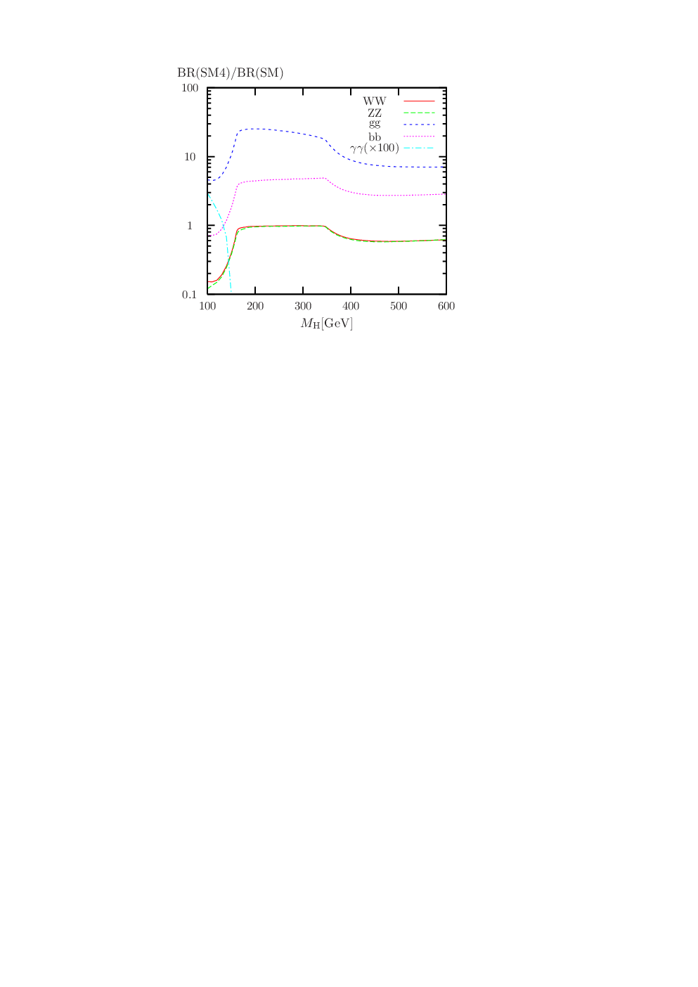
The results of the Higgs branching fractions for the scenarios defined in (2.2)/(2.3) are shown in Table 8 for the 2-fermion final states and in Table 9 for the 2-gauge-boson final states. In the latter table also the total Higgs width is given. Table 10 lists the branching fractions for the e+​e−​e+​e−{\mathrm{e^{+}}}{\mathrm{e^{-}}}{\mathrm{e^{+}}}{\mathrm{e^{-}}} and e+​e−​μ+​μ−{\mathrm{e^{+}}}{\mathrm{e^{-}}}\mu^{+}\mu^{-} final states as well as several combined channels. Apart from the sum of all 4-fermion final states (H→4​f{\mathrm{H}}\to 4f) the results for all-leptonic final states H→4​l{\mathrm{H}}\to 4l with l=e,μ,τ,νe,νμ,ντl={\mathrm{e}},\mu,\tau,\nu_{{\mathrm{e}}},\nu_{\mu},\nu_{\tau}, the results for all-hadronic final states H→4​q{\mathrm{H}}\to 4{q} with q=u,d,c,s,b{q}={\mathrm{u}},{\mathrm{d}},{\mathrm{c}},{\mathrm{s}},{\mathrm{b}} and the semi-leptonic final states H→2​l​2​q{\mathrm{H}}\to 2l2{q} are shown. To compare with the pure SM3, Fig. 4 shows the ratios between the SM4 and SM3 branching fractions for the most important channels for the scenario (2.4).

Table 8: SM4 Higgs branching fractions for 2-fermion decay channels for the scenarios defined in (2.2)/(2.3).

MHM_{{\mathrm{H}}} / mb′m_{{\mathrm{b^{\prime}}}}/ mνl′m_{\nu_{{\mathrm{l^{\prime}}}}} H→b​b¯{\mathrm{H}}\to{\mathrm{b}}\bar{{\mathrm{b}}} H→τ+​τ−{\mathrm{H}}\to\tau^{+}\tau^{-} H→μ+​μ−{\mathrm{H}}\to\mu^{+}\mu^{-} H→s​s¯{\mathrm{H}}\to{\mathrm{s}}\bar{{\mathrm{s}}} H→c​c¯{\mathrm{H}}\to{\mathrm{c}}\bar{{\mathrm{c}}} H→t​t¯{\mathrm{H}}\to{\mathrm{t}}\bar{{\mathrm{t}}} [GeV] 120/ 450/ 350 4.39⋅10−14.39\cdot 10^{-1} 4.77⋅10−24.77\cdot 10^{-2} 1.65⋅10−41.65\cdot 10^{-4} 1.87⋅10−41.87\cdot 10^{-4} 2.21⋅10−22.21\cdot 10^{-2} 0.000.00 120/ 450/ 375 4.39⋅10−14.39\cdot 10^{-1} 4.77⋅10−24.77\cdot 10^{-2} 1.66⋅10−41.66\cdot 10^{-4} 1.87⋅10−41.87\cdot 10^{-4} 2.22⋅10−22.22\cdot 10^{-2} 0.000.00 120/ 450/ 400 4.39⋅10−14.39\cdot 10^{-1} 4.77⋅10−24.77\cdot 10^{-2} 1.66⋅10−41.66\cdot 10^{-4} 1.87⋅10−41.87\cdot 10^{-4} 2.22⋅10−22.22\cdot 10^{-2} 0.000.00 120/ 500/ 350 4.45⋅10−14.45\cdot 10^{-1} 4.83⋅10−24.83\cdot 10^{-2} 1.68⋅10−41.68\cdot 10^{-4} 1.90⋅10−41.90\cdot 10^{-4} 2.24⋅10−22.24\cdot 10^{-2} 0.000.00 120/ 500/ 375 4.45⋅10−14.45\cdot 10^{-1} 4.84⋅10−24.84\cdot 10^{-2} 1.68⋅10−41.68\cdot 10^{-4} 1.90⋅10−41.90\cdot 10^{-4} 2.25⋅10−22.25\cdot 10^{-2} 0.000.00 120/ 500/ 400 4.45⋅10−14.45\cdot 10^{-1} 4.84⋅10−24.84\cdot 10^{-2} 1.68⋅10−41.68\cdot 10^{-4} 1.90⋅10−41.90\cdot 10^{-4} 2.25⋅10−22.25\cdot 10^{-2} 0.000.00 120/ 550/ 350 4.52⋅10−14.52\cdot 10^{-1} 4.91⋅10−24.91\cdot 10^{-2} 1.70⋅10−41.70\cdot 10^{-4} 1.93⋅10−41.93\cdot 10^{-4} 2.28⋅10−22.28\cdot 10^{-2} 0.000.00 120/ 550/ 375 4.52⋅10−14.52\cdot 10^{-1} 4.91⋅10−24.91\cdot 10^{-2} 1.70⋅10−41.70\cdot 10^{-4} 1.93⋅10−41.93\cdot 10^{-4} 2.28⋅10−22.28\cdot 10^{-2} 0.000.00 120/ 550/ 400 4.52⋅10−14.52\cdot 10^{-1} 4.92⋅10−24.92\cdot 10^{-2} 1.71⋅10−41.71\cdot 10^{-4} 1.93⋅10−41.93\cdot 10^{-4} 2.28⋅10−22.28\cdot 10^{-2} 0.000.00 350/ 450/ 350 7.25⋅10−47.25\cdot 10^{-4} 9.60⋅10−59.60\cdot 10^{-5} 3.33⋅10−73.33\cdot 10^{-7} 3.09⋅10−73.09\cdot 10^{-7} 3.64⋅10−53.64\cdot 10^{-5} 3.14⋅10−23.14\cdot 10^{-2} 350/ 450/ 375 7.32⋅10−47.32\cdot 10^{-4} 9.68⋅10−59.68\cdot 10^{-5} 3.36⋅10−73.36\cdot 10^{-7} 3.12⋅10−73.12\cdot 10^{-7} 3.68⋅10−53.68\cdot 10^{-5} 3.17⋅10−23.17\cdot 10^{-2} 350/ 450/ 400 7.39⋅10−47.39\cdot 10^{-4} 9.78⋅10−59.78\cdot 10^{-5} 3.39⋅10−73.39\cdot 10^{-7} 3.15⋅10−73.15\cdot 10^{-7} 3.71⋅10−53.71\cdot 10^{-5} 3.20⋅10−23.20\cdot 10^{-2} 350/ 500/ 350 7.72⋅10−47.72\cdot 10^{-4} 1.02⋅10−41.02\cdot 10^{-4} 3.54⋅10−73.54\cdot 10^{-7} 3.29⋅10−73.29\cdot 10^{-7} 3.88⋅10−53.88\cdot 10^{-5} 3.35⋅10−23.35\cdot 10^{-2} 350/ 500/ 375 7.79⋅10−47.79\cdot 10^{-4} 1.03⋅10−41.03\cdot 10^{-4} 3.57⋅10−73.57\cdot 10^{-7} 3.32⋅10−73.32\cdot 10^{-7} 3.92⋅10−53.92\cdot 10^{-5} 3.38⋅10−23.38\cdot 10^{-2} 350/ 500/ 400 7.87⋅10−47.87\cdot 10^{-4} 1.04⋅10−41.04\cdot 10^{-4} 3.61⋅10−73.61\cdot 10^{-7} 3.35⋅10−73.35\cdot 10^{-7} 3.95⋅10−53.95\cdot 10^{-5} 3.41⋅10−23.41\cdot 10^{-2} 350/ 550/ 350 8.36⋅10−48.36\cdot 10^{-4} 1.11⋅10−41.11\cdot 10^{-4} 3.83⋅10−73.83\cdot 10^{-7} 3.56⋅10−73.56\cdot 10^{-7} 4.20⋅10−54.20\cdot 10^{-5} 3.62⋅10−23.62\cdot 10^{-2} 350/ 550/ 375 8.44⋅10−48.44\cdot 10^{-4} 1.12⋅10−41.12\cdot 10^{-4} 3.87⋅10−73.87\cdot 10^{-7} 3.59⋅10−73.59\cdot 10^{-7} 4.24⋅10−54.24\cdot 10^{-5} 3.66⋅10−23.66\cdot 10^{-2} 350/ 550/ 400 8.53⋅10−48.53\cdot 10^{-4} 1.13⋅10−41.13\cdot 10^{-4} 3.91⋅10−73.91\cdot 10^{-7} 3.63⋅10−73.63\cdot 10^{-7} 4.28⋅10−54.28\cdot 10^{-5} 3.70⋅10−23.70\cdot 10^{-2} 600/ 450/ 300 1.24⋅10−41.24\cdot 10^{-4} 1.80⋅10−51.80\cdot 10^{-5} 6.25⋅10−86.25\cdot 10^{-8} 5.26⋅10−85.26\cdot 10^{-8} 6.20⋅10−66.20\cdot 10^{-6} 2.97⋅10−12.97\cdot 10^{-1} 600/ 450/ 350 1.22⋅10−41.22\cdot 10^{-4} 1.78⋅10−51.78\cdot 10^{-5} 6.17⋅10−86.17\cdot 10^{-8} 5.19⋅10−85.19\cdot 10^{-8} 6.12⋅10−66.12\cdot 10^{-6} 2.93⋅10−12.93\cdot 10^{-1} 600/ 450/ 400 1.23⋅10−41.23\cdot 10^{-4} 1.80⋅10−51.80\cdot 10^{-5} 6.24⋅10−86.24\cdot 10^{-8} 5.24⋅10−85.24\cdot 10^{-8} 6.18⋅10−66.18\cdot 10^{-6} 2.96⋅10−12.96\cdot 10^{-1} 600/ 500/ 300 1.29⋅10−41.29\cdot 10^{-4} 1.88⋅10−51.88\cdot 10^{-5} 6.51⋅10−86.51\cdot 10^{-8} 5.49⋅10−85.49\cdot 10^{-8} 6.47⋅10−66.47\cdot 10^{-6} 3.10⋅10−13.10\cdot 10^{-1} 600/ 500/ 350 1.27⋅10−41.27\cdot 10^{-4} 1.86⋅10−51.86\cdot 10^{-5} 6.43⋅10−86.43\cdot 10^{-8} 5.42⋅10−85.42\cdot 10^{-8} 6.39⋅10−66.39\cdot 10^{-6} 3.06⋅10−13.06\cdot 10^{-1} 600/ 500/ 400 1.29⋅10−41.29\cdot 10^{-4} 1.88⋅10−51.88\cdot 10^{-5} 6.50⋅10−86.50\cdot 10^{-8} 5.48⋅10−85.48\cdot 10^{-8} 6.46⋅10−66.46\cdot 10^{-6} 3.09⋅10−13.09\cdot 10^{-1} 600/ 550/ 300 1.36⋅10−41.36\cdot 10^{-4} 1.98⋅10−51.98\cdot 10^{-5} 6.87⋅10−86.87\cdot 10^{-8} 5.80⋅10−85.80\cdot 10^{-8} 6.84⋅10−66.84\cdot 10^{-6} 3.27⋅10−13.27\cdot 10^{-1} 600/ 550/ 350 1.35⋅10−41.35\cdot 10^{-4} 1.96⋅10−51.96\cdot 10^{-5} 6.78⋅10−86.78\cdot 10^{-8} 5.72⋅10−85.72\cdot 10^{-8} 6.75⋅10−66.75\cdot 10^{-6} 3.23⋅10−13.23\cdot 10^{-1} 600/ 550/ 400 1.36⋅10−41.36\cdot 10^{-4} 1.98⋅10−51.98\cdot 10^{-5} 6.85⋅10−86.85\cdot 10^{-8} 5.78⋅10−85.78\cdot 10^{-8} 6.82⋅10−66.82\cdot 10^{-6} 3.26⋅10−13.26\cdot 10^{-1}

Table 9: SM4 Higgs branching fractions for 2-gauge-boson decay channels and total Higgs width for the scenarios defined in (2.2)/(2.3).

MHM_{{\mathrm{H}}} / mb′m_{{\mathrm{b^{\prime}}}}/ mνl′m_{\nu_{{\mathrm{l^{\prime}}}}} H→gg{\mathrm{H}}\to{\mathrm{g}}{\mathrm{g}} H→Z​γ{\mathrm{H}}\to{\mathrm{Z}}\gamma H→WW{\mathrm{H}}\to{\mathrm{W}}{\mathrm{W}} H→ZZ{\mathrm{H}}\to{\mathrm{Z}}{\mathrm{Z}} ΓH\Gamma_{{\mathrm{H}}} [GeV] [GeV] 120/ 450/ 350 4.39⋅10−14.39\cdot 10^{-1} 4.54⋅10−44.54\cdot 10^{-4} 4.70⋅10−24.70\cdot 10^{-2} 5.14⋅10−35.14\cdot 10^{-3} 6.68⋅10−36.68\cdot 10^{-3} 120/ 450/ 375 4.39⋅10−14.39\cdot 10^{-1} 4.54⋅10−44.54\cdot 10^{-4} 4.66⋅10−24.66\cdot 10^{-2} 5.10⋅10−35.10\cdot 10^{-3} 6.69⋅10−36.69\cdot 10^{-3} 120/ 450/ 400 4.39⋅10−14.39\cdot 10^{-1} 4.53⋅10−44.53\cdot 10^{-4} 4.62⋅10−24.62\cdot 10^{-2} 5.05⋅10−35.05\cdot 10^{-3} 6.70⋅10−36.70\cdot 10^{-3} 120/ 500/ 350 4.34⋅10−14.34\cdot 10^{-1} 4.51⋅10−44.51\cdot 10^{-4} 4.47⋅10−24.47\cdot 10^{-2} 4.88⋅10−34.88\cdot 10^{-3} 6.74⋅10−36.74\cdot 10^{-3} 120/ 500/ 375 4.35⋅10−14.35\cdot 10^{-1} 4.50⋅10−44.50\cdot 10^{-4} 4.43⋅10−24.43\cdot 10^{-2} 4.84⋅10−34.84\cdot 10^{-3} 6.75⋅10−36.75\cdot 10^{-3} 120/ 500/ 400 4.35⋅10−14.35\cdot 10^{-1} 4.50⋅10−44.50\cdot 10^{-4} 4.38⋅10−24.38\cdot 10^{-2} 4.79⋅10−34.79\cdot 10^{-3} 6.76⋅10−36.76\cdot 10^{-3} 120/ 550/ 350 4.29⋅10−14.29\cdot 10^{-1} 4.45⋅10−44.45\cdot 10^{-4} 4.19⋅10−24.19\cdot 10^{-2} 4.55⋅10−34.55\cdot 10^{-3} 6.82⋅10−36.82\cdot 10^{-3} 120/ 550/ 375 4.29⋅10−14.29\cdot 10^{-1} 4.45⋅10−44.45\cdot 10^{-4} 4.15⋅10−24.15\cdot 10^{-2} 4.51⋅10−34.51\cdot 10^{-3} 6.83⋅10−36.83\cdot 10^{-3} 120/ 550/ 400 4.30⋅10−14.30\cdot 10^{-1} 4.44⋅10−44.44\cdot 10^{-4} 4.10⋅10−24.10\cdot 10^{-2} 4.46⋅10−34.46\cdot 10^{-3} 6.84⋅10−36.84\cdot 10^{-3} 350/ 450/ 350 6.91⋅10−36.91\cdot 10^{-3} 5.54⋅10−55.54\cdot 10^{-5} 6.62⋅10−16.62\cdot 10^{-1} 2.99⋅10−12.99\cdot 10^{-1} 9.729.72 350/ 450/ 375 6.97⋅10−36.97\cdot 10^{-3} 5.58⋅10−55.58\cdot 10^{-5} 6.62⋅10−16.62\cdot 10^{-1} 2.98⋅10−12.98\cdot 10^{-1} 9.659.65 350/ 450/ 400 7.04⋅10−37.04\cdot 10^{-3} 5.62⋅10−55.62\cdot 10^{-5} 6.61⋅10−16.61\cdot 10^{-1} 2.98⋅10−12.98\cdot 10^{-1} 9.589.58 350/ 500/ 350 7.17⋅10−37.17\cdot 10^{-3} 5.77⋅10−55.77\cdot 10^{-5} 6.60⋅10−16.60\cdot 10^{-1} 2.98⋅10−12.98\cdot 10^{-1} 9.339.33 350/ 500/ 375 7.24⋅10−37.24\cdot 10^{-3} 5.81⋅10−55.81\cdot 10^{-5} 6.60⋅10−16.60\cdot 10^{-1} 2.98⋅10−12.98\cdot 10^{-1} 9.269.26 350/ 500/ 400 7.31⋅10−37.31\cdot 10^{-3} 5.86⋅10−55.86\cdot 10^{-5} 6.59⋅10−16.59\cdot 10^{-1} 2.98⋅10−12.98\cdot 10^{-1} 9.199.19 350/ 550/ 350 7.54⋅10−37.54\cdot 10^{-3} 6.07⋅10−56.07\cdot 10^{-5} 6.58⋅10−16.58\cdot 10^{-1} 2.97⋅10−12.97\cdot 10^{-1} 8.878.87 350/ 550/ 375 7.62⋅10−37.62\cdot 10^{-3} 6.12⋅10−56.12\cdot 10^{-5} 6.58⋅10−16.58\cdot 10^{-1} 2.96⋅10−12.96\cdot 10^{-1} 8.808.80 350/ 550/ 400 7.70⋅10−37.70\cdot 10^{-3} 6.17⋅10−56.17\cdot 10^{-5} 6.58⋅10−16.58\cdot 10^{-1} 2.96⋅10−12.96\cdot 10^{-1} 8.738.73 600/ 450/ 300 2.27⋅10−32.27\cdot 10^{-3} 6.52⋅10−66.52\cdot 10^{-6} 4.71⋅10−14.71\cdot 10^{-1} 2.30⋅10−12.30\cdot 10^{-1} 8.96⋅1018.96\cdot 10^{1} 600/ 450/ 350 2.32⋅10−32.32\cdot 10^{-3} 6.43⋅10−66.43\cdot 10^{-6} 4.73⋅10−14.73\cdot 10^{-1} 2.31⋅10−12.31\cdot 10^{-1} 9.09⋅1019.09\cdot 10^{1} 600/ 450/ 400 2.36⋅10−32.36\cdot 10^{-3} 6.47⋅10−66.47\cdot 10^{-6} 4.71⋅10−14.71\cdot 10^{-1} 2.30⋅10−12.30\cdot 10^{-1} 9.03⋅1019.03\cdot 10^{1} 600/ 500/ 300 2.27⋅10−32.27\cdot 10^{-3} 6.62⋅10−66.62\cdot 10^{-6} 4.62⋅10−14.62\cdot 10^{-1} 2.26⋅10−12.26\cdot 10^{-1} 8.78⋅1018.78\cdot 10^{1} 600/ 500/ 350 2.31⋅10−32.31\cdot 10^{-3} 6.53⋅10−66.53\cdot 10^{-6} 4.65⋅10−14.65\cdot 10^{-1} 2.27⋅10−12.27\cdot 10^{-1} 8.92⋅1018.92\cdot 10^{1} 600/ 500/ 400 2.35⋅10−32.35\cdot 10^{-3} 6.57⋅10−66.57\cdot 10^{-6} 4.63⋅10−14.63\cdot 10^{-1} 2.26⋅10−12.26\cdot 10^{-1} 8.86⋅1018.86\cdot 10^{1} 600/ 550/ 300 2.29⋅10−32.29\cdot 10^{-3} 6.77⋅10−66.77\cdot 10^{-6} 4.51⋅10−14.51\cdot 10^{-1} 2.20⋅10−12.20\cdot 10^{-1} 8.57⋅1018.57\cdot 10^{1} 600/ 550/ 350 2.34⋅10−32.34\cdot 10^{-3} 6.67⋅10−66.67\cdot 10^{-6} 4.54⋅10−14.54\cdot 10^{-1} 2.21⋅10−12.21\cdot 10^{-1} 8.70⋅1018.70\cdot 10^{1} 600/ 550/ 400 2.38⋅10−32.38\cdot 10^{-3} 6.71⋅10−66.71\cdot 10^{-6} 4.51⋅10−14.51\cdot 10^{-1} 2.20⋅10−12.20\cdot 10^{-1} 8.64⋅1018.64\cdot 10^{1}

Table 10: SM4 Higgs branching fractions for 4-fermion final states with l=e,μ,τ,νe,νμ,ντl={\mathrm{e}},\mu,\tau,\nu_{{\mathrm{e}}},\nu_{\mu},\,\nu_{\tau} and q=u,d,c,s,b{q}={\mathrm{u}},{\mathrm{d}},{\mathrm{c}},{\mathrm{s}},{\mathrm{b}} for the scenarios defined in (2.2)/(2.3).

MHM_{{\mathrm{H}}} / mb′m_{{\mathrm{b^{\prime}}}}/ mνl′m_{\nu_{{\mathrm{l^{\prime}}}}} H→4​e{\mathrm{H}}\to 4{\mathrm{e}} H→2​e​2​μ{\mathrm{H}}\to 2{\mathrm{e}}2\mu H→4​l{\mathrm{H}}\to 4l H→4​q{\mathrm{H}}\to 4{q} H→2​l​2​q{\mathrm{H}}\to 2l2{q} H→4​f{\mathrm{H}}\to 4f [GeV] 120/ 450/ 350 6.39⋅10−66.39\cdot 10^{-6} 1.14⋅10−51.14\cdot 10^{-5} 5.24⋅10−35.24\cdot 10^{-3} 2.38⋅10−22.38\cdot 10^{-2} 2.27⋅10−22.27\cdot 10^{-2} 5.17⋅10−25.17\cdot 10^{-2} 120/ 450/ 375 6.33⋅10−66.33\cdot 10^{-6} 1.13⋅10−51.13\cdot 10^{-5} 5.19⋅10−35.19\cdot 10^{-3} 2.36⋅10−22.36\cdot 10^{-2} 2.25⋅10−22.25\cdot 10^{-2} 5.12⋅10−25.12\cdot 10^{-2} 120/ 450/ 400 6.27⋅10−66.27\cdot 10^{-6} 1.12⋅10−51.12\cdot 10^{-5} 5.14⋅10−35.14\cdot 10^{-3} 2.33⋅10−22.33\cdot 10^{-2} 2.23⋅10−22.23\cdot 10^{-2} 5.08⋅10−25.08\cdot 10^{-2} 120/ 500/ 350 6.05⋅10−66.05\cdot 10^{-6} 1.08⋅10−51.08\cdot 10^{-5} 4.96⋅10−34.96\cdot 10^{-3} 2.26⋅10−22.26\cdot 10^{-2} 2.15⋅10−22.15\cdot 10^{-2} 4.91⋅10−24.91\cdot 10^{-2} 120/ 500/ 375 5.99⋅10−65.99\cdot 10^{-6} 1.07⋅10−51.07\cdot 10^{-5} 4.91⋅10−34.91\cdot 10^{-3} 2.24⋅10−22.24\cdot 10^{-2} 2.13⋅10−22.13\cdot 10^{-2} 4.87⋅10−24.87\cdot 10^{-2} 120/ 500/ 400 5.93⋅10−65.93\cdot 10^{-6} 1.06⋅10−51.06\cdot 10^{-5} 4.86⋅10−34.86\cdot 10^{-3} 2.22⋅10−22.22\cdot 10^{-2} 2.11⋅10−22.11\cdot 10^{-2} 4.82⋅10−24.82\cdot 10^{-2} 120/ 550/ 350 5.62⋅10−65.62\cdot 10^{-6} 1.00⋅10−51.00\cdot 10^{-5} 4.63⋅10−34.63\cdot 10^{-3} 2.12⋅10−22.12\cdot 10^{-2} 2.02⋅10−22.02\cdot 10^{-2} 4.60⋅10−24.60\cdot 10^{-2} 120/ 550/ 375 5.56⋅10−65.56\cdot 10^{-6} 9.93⋅10−69.93\cdot 10^{-6} 4.58⋅10−34.58\cdot 10^{-3} 2.10⋅10−22.10\cdot 10^{-2} 2.00⋅10−22.00\cdot 10^{-2} 4.56⋅10−24.56\cdot 10^{-2} 120/ 550/ 400 5.50⋅10−65.50\cdot 10^{-6} 9.82⋅10−69.82\cdot 10^{-6} 4.53⋅10−34.53\cdot 10^{-3} 2.08⋅10−22.08\cdot 10^{-2} 1.98⋅10−21.98\cdot 10^{-2} 4.51⋅10−24.51\cdot 10^{-2} 350/ 450/ 350 3.25⋅10−43.25\cdot 10^{-4} 6.52⋅10−46.52\cdot 10^{-4} 9.47⋅10−29.47\cdot 10^{-2} 4.52⋅10−14.52\cdot 10^{-1} 4.14⋅10−14.14\cdot 10^{-1} 9.61⋅10−19.61\cdot 10^{-1} 350/ 450/ 375 3.25⋅10−43.25\cdot 10^{-4} 6.52⋅10−46.52\cdot 10^{-4} 9.46⋅10−29.46\cdot 10^{-2} 4.52⋅10−14.52\cdot 10^{-1} 4.14⋅10−14.14\cdot 10^{-1} 9.60⋅10−19.60\cdot 10^{-1} 350/ 450/ 400 3.24⋅10−43.24\cdot 10^{-4} 6.51⋅10−46.51\cdot 10^{-4} 9.45⋅10−29.45\cdot 10^{-2} 4.52⋅10−14.52\cdot 10^{-1} 4.13⋅10−14.13\cdot 10^{-1} 9.60⋅10−19.60\cdot 10^{-1} 350/ 500/ 350 3.23⋅10−43.23\cdot 10^{-4} 6.48⋅10−46.48\cdot 10^{-4} 9.41⋅10−29.41\cdot 10^{-2} 4.52⋅10−14.52\cdot 10^{-1} 4.12⋅10−14.12\cdot 10^{-1} 9.58⋅10−19.58\cdot 10^{-1} 350/ 500/ 375 3.23⋅10−43.23\cdot 10^{-4} 6.48⋅10−46.48\cdot 10^{-4} 9.40⋅10−29.40\cdot 10^{-2} 4.52⋅10−14.52\cdot 10^{-1} 4.12⋅10−14.12\cdot 10^{-1} 9.58⋅10−19.58\cdot 10^{-1} 350/ 500/ 400 3.22⋅10−43.22\cdot 10^{-4} 6.47⋅10−46.47\cdot 10^{-4} 9.39⋅10−29.39\cdot 10^{-2} 4.52⋅10−14.52\cdot 10^{-1} 4.12⋅10−14.12\cdot 10^{-1} 9.58⋅10−19.58\cdot 10^{-1} 350/ 550/ 350 3.20⋅10−43.20\cdot 10^{-4} 6.43⋅10−46.43\cdot 10^{-4} 9.35⋅10−29.35\cdot 10^{-2} 4.51⋅10−14.51\cdot 10^{-1} 4.11⋅10−14.11\cdot 10^{-1} 9.55⋅10−19.55\cdot 10^{-1} 350/ 550/ 375 3.20⋅10−43.20\cdot 10^{-4} 6.42⋅10−46.42\cdot 10^{-4} 9.33⋅10−29.33\cdot 10^{-2} 4.51⋅10−14.51\cdot 10^{-1} 4.10⋅10−14.10\cdot 10^{-1} 9.55⋅10−19.55\cdot 10^{-1} 350/ 550/ 400 3.19⋅10−43.19\cdot 10^{-4} 6.41⋅10−46.41\cdot 10^{-4} 9.32⋅10−29.32\cdot 10^{-2} 4.51⋅10−14.51\cdot 10^{-1} 4.10⋅10−14.10\cdot 10^{-1} 9.54⋅10−19.54\cdot 10^{-1} 600/ 450/ 300 2.52⋅10−42.52\cdot 10^{-4} 5.05⋅10−45.05\cdot 10^{-4} 6.92⋅10−26.92\cdot 10^{-2} 3.29⋅10−13.29\cdot 10^{-1} 3.02⋅10−13.02\cdot 10^{-1} 7.00⋅10−17.00\cdot 10^{-1} 600/ 450/ 350 2.53⋅10−42.53\cdot 10^{-4} 5.07⋅10−45.07\cdot 10^{-4} 6.96⋅10−26.96\cdot 10^{-2} 3.31⋅10−13.31\cdot 10^{-1} 3.04⋅10−13.04\cdot 10^{-1} 7.04⋅10−17.04\cdot 10^{-1} 600/ 450/ 400 2.52⋅10−42.52\cdot 10^{-4} 5.05⋅10−45.05\cdot 10^{-4} 6.92⋅10−26.92\cdot 10^{-2} 3.30⋅10−13.30\cdot 10^{-1} 3.02⋅10−13.02\cdot 10^{-1} 7.01⋅10−17.01\cdot 10^{-1} 600/ 500/ 300 2.47⋅10−42.47\cdot 10^{-4} 4.95⋅10−44.95\cdot 10^{-4} 6.77⋅10−26.77\cdot 10^{-2} 3.24⋅10−13.24\cdot 10^{-1} 2.96⋅10−12.96\cdot 10^{-1} 6.88⋅10−16.88\cdot 10^{-1} 600/ 500/ 350 2.48⋅10−42.48\cdot 10^{-4} 4.97⋅10−44.97\cdot 10^{-4} 6.81⋅10−26.81\cdot 10^{-2} 3.26⋅10−13.26\cdot 10^{-1} 2.98⋅10−12.98\cdot 10^{-1} 6.92⋅10−16.92\cdot 10^{-1} 600/ 500/ 400 2.47⋅10−42.47\cdot 10^{-4} 4.94⋅10−44.94\cdot 10^{-4} 6.77⋅10−26.77\cdot 10^{-2} 3.24⋅10−13.24\cdot 10^{-1} 2.96⋅10−12.96\cdot 10^{-1} 6.88⋅10−16.88\cdot 10^{-1} 600/ 550/ 300 2.40⋅10−42.40\cdot 10^{-4} 4.81⋅10−44.81\cdot 10^{-4} 6.58⋅10−26.58\cdot 10^{-2} 3.16⋅10−13.16\cdot 10^{-1} 2.89⋅10−12.89\cdot 10^{-1} 6.71⋅10−16.71\cdot 10^{-1} 600/ 550/ 350 2.41⋅10−42.41\cdot 10^{-4} 4.83⋅10−44.83\cdot 10^{-4} 6.63⋅10−26.63\cdot 10^{-2} 3.18⋅10−13.18\cdot 10^{-1} 2.91⋅10−12.91\cdot 10^{-1} 6.75⋅10−16.75\cdot 10^{-1} 600/ 550/ 400 2.40⋅10−42.40\cdot 10^{-4} 4.80⋅10−44.80\cdot 10^{-4} 6.58⋅10−26.58\cdot 10^{-2} 3.17⋅10−13.17\cdot 10^{-1} 2.89⋅10−12.89\cdot 10^{-1} 6.71⋅10−16.71\cdot 10^{-1}

Refer to caption

Figure 4: Ratio of branching fractions in SM4 with respect to SM3 for WW{\mathrm{W}}{\mathrm{W}}, ZZ{\mathrm{Z}}{\mathrm{Z}}, gg{\mathrm{g}}{\mathrm{g}}, b​b¯{\mathrm{b}}\bar{{\mathrm{b}}}, and γ​γ\gamma\gamma decay channels (γ​γ\gamma\gamma ratio multiplied with 100100) as a function of MHM_{{\mathrm{H}}} for scenario (2.4).

While the branching ratio into gluons is enhanced by a factor 5−155{-}15, BR⁡(H→b​b¯){\mathrm{BR}}({\mathrm{H}}\to{\mathrm{b}}\bar{\mathrm{b}}) is reduced for small MHM_{{\mathrm{H}}} but enhanced for MH∼> 150​GeVM_{{\mathrm{H}}}\;\raisebox{-3.00003pt}{$\stackrel{{\scriptstyle\displaystyle>}}{{\sim}}$}\;150\,\mathrm{GeV}. The branching ratios into electroweak gauge-boson pairs are suppressed for small Higgs masses, and the one into photon pairs is reduced by 6565 to 100%100\% in the Higgs-mass range 100​GeV<MH<150​GeV100\,\mathrm{GeV}<M_{{\mathrm{H}}}<150\,\mathrm{GeV}.

Results in the extreme scenario (2.5) for Higgs masses up to 1​TeV1\,\mathrm{TeV} are shown in Table 11 for the 2-fermion final states, in Table 12 for the 2-gauge-boson final states and the total Higgs width, and in Table 13 for selected 4-fermion final states. The ratios between the SM4 and SM3 branching fractions for the most important channels are shown in Fig. 5. As compared to the scenario of Fig. 4, the enhancement and suppression effects are stronger (as they scale roughly with the square of the heavy fermion masses). While BR⁡(H→γ​γ){\mathrm{BR}}({\mathrm{H}}\to\gamma\gamma) is different in detail it is again suppressed by a factor 100.

Table 11: SM4 Higgs branching fractions for 2-fermion decay channels in the extreme scenario (2.5).

MHM_{{\mathrm{H}}} [GeV] H→b​b¯{\mathrm{H}}\to{\mathrm{b}}\bar{{\mathrm{b}}} H→τ+​τ−{\mathrm{H}}\to\tau^{+}\tau^{-} H→μ+​μ−{\mathrm{H}}\to\mu^{+}\mu^{-} H→s​s¯{\mathrm{H}}\to{\mathrm{s}}\bar{{\mathrm{s}}} H→c​c¯{\mathrm{H}}\to{\mathrm{c}}\bar{{\mathrm{c}}} H→t​t¯{\mathrm{H}}\to{\mathrm{t}}\bar{{\mathrm{t}}} 100 5.70⋅10−15.70\cdot 10^{-1} 5.98⋅10−25.98\cdot 10^{-2} 2.08⋅10−42.08\cdot 10^{-4} 2.44⋅10−42.44\cdot 10^{-4} 2.88⋅10−22.88\cdot 10^{-2} 0.000.00 110 5.30⋅10−15.30\cdot 10^{-1} 5.67⋅10−25.67\cdot 10^{-2} 1.97⋅10−41.97\cdot 10^{-4} 2.26⋅10−42.26\cdot 10^{-4} 2.68⋅10−22.68\cdot 10^{-2} 0.000.00 120 4.87⋅10−14.87\cdot 10^{-1} 5.29⋅10−25.29\cdot 10^{-2} 1.84⋅10−41.84\cdot 10^{-4} 2.08⋅10−42.08\cdot 10^{-4} 2.46⋅10−22.46\cdot 10^{-2} 0.000.00 130 4.36⋅10−14.36\cdot 10^{-1} 4.82⋅10−24.82\cdot 10^{-2} 1.67⋅10−41.67\cdot 10^{-4} 1.86⋅10−41.86\cdot 10^{-4} 2.20⋅10−22.20\cdot 10^{-2} 0.000.00 140 3.72⋅10−13.72\cdot 10^{-1} 4.17⋅10−24.17\cdot 10^{-2} 1.45⋅10−41.45\cdot 10^{-4} 1.59⋅10−41.59\cdot 10^{-4} 1.88⋅10−21.88\cdot 10^{-2} 0.000.00 150 2.83⋅10−12.83\cdot 10^{-1} 3.20⋅10−23.20\cdot 10^{-2} 1.11⋅10−41.11\cdot 10^{-4} 1.21⋅10−41.21\cdot 10^{-4} 1.42⋅10−21.42\cdot 10^{-2} 0.000.00 160 1.13⋅10−11.13\cdot 10^{-1} 1.29⋅10−21.29\cdot 10^{-2} 4.48⋅10−54.48\cdot 10^{-5} 4.80⋅10−54.80\cdot 10^{-5} 5.67⋅10−35.67\cdot 10^{-3} 0.000.00 170 3.26⋅10−23.26\cdot 10^{-2} 3.78⋅10−33.78\cdot 10^{-3} 1.31⋅10−51.31\cdot 10^{-5} 1.39⋅10−51.39\cdot 10^{-5} 1.64⋅10−31.64\cdot 10^{-3} 0.000.00 180 2.15⋅10−22.15\cdot 10^{-2} 2.52⋅10−32.52\cdot 10^{-3} 8.74⋅10−68.74\cdot 10^{-6} 9.17⋅10−69.17\cdot 10^{-6} 1.08⋅10−31.08\cdot 10^{-3} 0.000.00 190 1.39⋅10−21.39\cdot 10^{-2} 1.64⋅10−31.64\cdot 10^{-3} 5.69⋅10−65.69\cdot 10^{-6} 5.91⋅10−65.91\cdot 10^{-6} 6.98⋅10−46.98\cdot 10^{-4} 0.000.00 200 1.06⋅10−21.06\cdot 10^{-2} 1.27⋅10−31.27\cdot 10^{-3} 4.41⋅10−64.41\cdot 10^{-6} 4.53⋅10−64.53\cdot 10^{-6} 5.35⋅10−45.35\cdot 10^{-4} 0.000.00 250 4.73⋅10−34.73\cdot 10^{-3} 5.89⋅10−45.89\cdot 10^{-4} 2.04⋅10−62.04\cdot 10^{-6} 2.01⋅10−62.01\cdot 10^{-6} 2.38⋅10−42.38\cdot 10^{-4} 0.000.00 300 2.70⋅10−32.70\cdot 10^{-3} 3.48⋅10−43.48\cdot 10^{-4} 1.21⋅10−61.21\cdot 10^{-6} 1.15⋅10−61.15\cdot 10^{-6} 1.36⋅10−41.36\cdot 10^{-4} 3.26⋅10−43.26\cdot 10^{-4} 400 6.38⋅10−46.38\cdot 10^{-4} 8.63⋅10−58.63\cdot 10^{-5} 2.99⋅10−72.99\cdot 10^{-7} 2.71⋅10−72.71\cdot 10^{-7} 3.20⋅10−53.20\cdot 10^{-5} 4.50⋅10−14.50\cdot 10^{-1} 500 2.96⋅10−42.96\cdot 10^{-4} 4.16⋅10−54.16\cdot 10^{-5} 1.44⋅10−71.44\cdot 10^{-7} 1.26⋅10−71.26\cdot 10^{-7} 1.48⋅10−51.48\cdot 10^{-5} 5.22⋅10−15.22\cdot 10^{-1} 600 2.02⋅10−42.02\cdot 10^{-4} 2.92⋅10−52.92\cdot 10^{-5} 1.01⋅10−71.01\cdot 10^{-7} 8.58⋅10−88.58\cdot 10^{-8} 1.01⋅10−51.01\cdot 10^{-5} 4.82⋅10−14.82\cdot 10^{-1} 700 1.52⋅10−41.52\cdot 10^{-4} 2.26⋅10−52.26\cdot 10^{-5} 7.82⋅10−87.82\cdot 10^{-8} 6.46⋅10−86.46\cdot 10^{-8} 7.61⋅10−67.61\cdot 10^{-6} 4.21⋅10−14.21\cdot 10^{-1} 800 1.18⋅10−41.18\cdot 10^{-4} 1.80⋅10−51.80\cdot 10^{-5} 6.24⋅10−86.24\cdot 10^{-8} 5.02⋅10−85.02\cdot 10^{-8} 5.91⋅10−65.91\cdot 10^{-6} 3.56⋅10−13.56\cdot 10^{-1} 1000 7.37⋅10−57.37\cdot 10^{-5} 1.17⋅10−51.17\cdot 10^{-5} 4.06⋅10−84.06\cdot 10^{-8} 3.13⋅10−83.13\cdot 10^{-8} 3.69⋅10−63.69\cdot 10^{-6} 2.43⋅10−12.43\cdot 10^{-1}

Table 12: SM4 Higgs branching fractions for 2-gauge-boson decay channels and total Higgs width in the extreme scenario (2.5).

MHM_{{\mathrm{H}}} [GeV] H→gg{\mathrm{H}}\to{\mathrm{g}}{\mathrm{g}} H→Z​γ{\mathrm{H}}\to{\mathrm{Z}}\gamma H→WW{\mathrm{H}}\to{\mathrm{W}}{\mathrm{W}} H→ZZ{\mathrm{H}}\to{\mathrm{Z}}{\mathrm{Z}} ΓH\Gamma_{{\mathrm{H}}} [GeV] 100 3.39⋅10−13.39\cdot 10^{-1} 1.70⋅10−51.70\cdot 10^{-5} 1.67⋅10−31.67\cdot 10^{-3} 1.35⋅10−41.35\cdot 10^{-4} 5.52⋅10−35.52\cdot 10^{-3} 110 3.78⋅10−13.78\cdot 10^{-1} 1.35⋅10−41.35\cdot 10^{-4} 7.20⋅10−37.20\cdot 10^{-3} 5.83⋅10−45.83\cdot 10^{-4} 6.41⋅10−36.41\cdot 10^{-3} 120 4.10⋅10−14.10\cdot 10^{-1} 4.06⋅10−44.06\cdot 10^{-4} 2.27⋅10−22.27\cdot 10^{-2} 2.37⋅10−32.37\cdot 10^{-3} 7.49⋅10−37.49\cdot 10^{-3} 130 4.28⋅10−14.28\cdot 10^{-1} 8.51⋅10−48.51\cdot 10^{-4} 5.77⋅10−25.77\cdot 10^{-2} 7.12⋅10−37.12\cdot 10^{-3} 8.92⋅10−38.92\cdot 10^{-3} 140 4.20⋅10−14.20\cdot 10^{-1} 1.46⋅10−31.46\cdot 10^{-3} 1.29⋅10−11.29\cdot 10^{-1} 1.68⋅10−21.68\cdot 10^{-2} 1.11⋅10−21.11\cdot 10^{-2} 150 3.63⋅10−13.63\cdot 10^{-1} 2.13⋅10−32.13\cdot 10^{-3} 2.75⋅10−12.75\cdot 10^{-1} 3.09⋅10−23.09\cdot 10^{-2} 1.55⋅10−21.55\cdot 10^{-2} 160 1.62⋅10−11.62\cdot 10^{-1} 2.01⋅10−32.01\cdot 10^{-3} 6.80⋅10−16.80\cdot 10^{-1} 2.78⋅10−22.78\cdot 10^{-2} 4.10⋅10−24.10\cdot 10^{-2} 170 5.27⋅10−25.27\cdot 10^{-2} 8.96⋅10−48.96\cdot 10^{-4} 8.90⋅10−18.90\cdot 10^{-1} 2.02⋅10−22.02\cdot 10^{-2} 1.49⋅10−11.49\cdot 10^{-1} 180 3.85⋅10−23.85\cdot 10^{-2} 6.95⋅10−46.95\cdot 10^{-4} 8.82⋅10−18.82\cdot 10^{-1} 5.43⋅10−25.43\cdot 10^{-2} 2.37⋅10−12.37\cdot 10^{-1} 190 2.75⋅10−22.75\cdot 10^{-2} 5.07⋅10−45.07\cdot 10^{-4} 7.60⋅10−17.60\cdot 10^{-1} 1.97⋅10−11.97\cdot 10^{-1} 3.84⋅10−13.84\cdot 10^{-1} 200 2.33⋅10−22.33\cdot 10^{-2} 4.28⋅10−44.28\cdot 10^{-4} 7.18⋅10−17.18\cdot 10^{-1} 2.43⋅10−12.43\cdot 10^{-1} 5.21⋅10−15.21\cdot 10^{-1} 250 1.62⋅10−21.62\cdot 10^{-2} 2.48⋅10−42.48\cdot 10^{-4} 6.93⋅10−16.93\cdot 10^{-1} 2.86⋅10−12.86\cdot 10^{-1} 1.411.41 300 1.39⋅10−21.39\cdot 10^{-2} 1.58⋅10−41.58\cdot 10^{-4} 6.84⋅10−16.84\cdot 10^{-1} 3.00⋅10−13.00\cdot 10^{-1} 2.872.87 400 7.40⋅10−37.40\cdot 10^{-3} 3.63⋅10−53.63\cdot 10^{-5} 3.74⋅10−13.74\cdot 10^{-1} 1.68⋅10−11.68\cdot 10^{-1} 1.55⋅1011.55\cdot 10^{1} 500 4.28⋅10−34.28\cdot 10^{-3} 1.41⋅10−51.41\cdot 10^{-5} 3.22⋅10−13.22\cdot 10^{-1} 1.51⋅10−11.51\cdot 10^{-1} 4.06⋅1014.06\cdot 10^{1} 600 2.99⋅10−32.99\cdot 10^{-3} 8.21⋅10−68.21\cdot 10^{-6} 3.46⋅10−13.46\cdot 10^{-1} 1.69⋅10−11.69\cdot 10^{-1} 6.99⋅1016.99\cdot 10^{1} 700 2.17⋅10−32.17\cdot 10^{-3} 5.46⋅10−65.46\cdot 10^{-6} 3.86⋅10−13.86\cdot 10^{-1} 1.91⋅10−11.91\cdot 10^{-1} 1.06⋅1021.06\cdot 10^{2} 800 1.60⋅10−31.60\cdot 10^{-3} 3.88⋅10−63.88\cdot 10^{-6} 4.27⋅10−14.27\cdot 10^{-1} 2.15⋅10−12.15\cdot 10^{-1} 1.52⋅1021.52\cdot 10^{2} 1000 8.08⋅10−48.08\cdot 10^{-4} 2.28⋅10−62.28\cdot 10^{-6} 5.02⋅10−15.02\cdot 10^{-1} 2.54⋅10−12.54\cdot 10^{-1} 2.88⋅1022.88\cdot 10^{2}

Table 13: SM4 Higgs branching fractions for 4-fermion final states with l=e,μ,τ,νe,νμ,ντl={\mathrm{e}},\mu,\tau,\nu_{{\mathrm{e}}},\nu_{\mu},\,\nu_{\tau} and q=u,d,c,s,b{q}={\mathrm{u}},{\mathrm{d}},{\mathrm{c}},{\mathrm{s}},{\mathrm{b}} in the extreme scenario (2.5).

MHM_{{\mathrm{H}}} [GeV] H→4​e{\mathrm{H}}\to 4{\mathrm{e}} H→2​e​2​μ{\mathrm{H}}\to 2{\mathrm{e}}2\mu H→4​l{\mathrm{H}}\to 4l H→4​q{\mathrm{H}}\to 4{q} H→2​l​2​q{\mathrm{H}}\to 2l2{q} H→4​f{\mathrm{H}}\to 4f 100 2.26⋅10−72.26\cdot 10^{-7} 3.31⋅10−73.31\cdot 10^{-7} 1.67⋅10−41.67\cdot 10^{-4} 7.48⋅10−47.48\cdot 10^{-4} 7.85⋅10−47.85\cdot 10^{-4} 1.70⋅10−31.70\cdot 10^{-3} 110 7.81⋅10−77.81\cdot 10^{-7} 1.27⋅10−61.27\cdot 10^{-6} 7.32⋅10−47.32\cdot 10^{-4} 3.53⋅10−33.53\cdot 10^{-3} 3.36⋅10−33.36\cdot 10^{-3} 7.62⋅10−37.62\cdot 10^{-3} 120 2.76⋅10−62.76\cdot 10^{-6} 4.99⋅10−64.99\cdot 10^{-6} 2.36⋅10−32.36\cdot 10^{-3} 1.17⋅10−21.17\cdot 10^{-2} 1.08⋅10−21.08\cdot 10^{-2} 2.48⋅10−22.48\cdot 10^{-2} 130 8.00⋅10−68.00\cdot 10^{-6} 1.48⋅10−51.48\cdot 10^{-5} 6.12⋅10−36.12\cdot 10^{-3} 3.05⋅10−23.05\cdot 10^{-2} 2.78⋅10−22.78\cdot 10^{-2} 6.44⋅10−26.44\cdot 10^{-2} 140 1.83⋅10−51.83\cdot 10^{-5} 3.51⋅10−53.51\cdot 10^{-5} 1.38⋅10−21.38\cdot 10^{-2} 6.88⋅10−26.88\cdot 10^{-2} 6.24⋅10−26.24\cdot 10^{-2} 1.45⋅10−11.45\cdot 10^{-1} 150 3.33⋅10−53.33\cdot 10^{-5} 6.42⋅10−56.42\cdot 10^{-5} 2.91⋅10−22.91\cdot 10^{-2} 1.45⋅10−11.45\cdot 10^{-1} 1.31⋅10−11.31\cdot 10^{-1} 3.05⋅10−13.05\cdot 10^{-1} 160 2.95⋅10−52.95\cdot 10^{-5} 5.75⋅10−55.75\cdot 10^{-5} 6.85⋅10−26.85\cdot 10^{-2} 3.31⋅10−13.31\cdot 10^{-1} 3.05⋅10−13.05\cdot 10^{-1} 7.04⋅10−17.04\cdot 10^{-1} 170 2.13⋅10−52.13\cdot 10^{-5} 4.17⋅10−54.17\cdot 10^{-5} 8.81⋅10−28.81\cdot 10^{-2} 4.29⋅10−14.29\cdot 10^{-1} 3.92⋅10−13.92\cdot 10^{-1} 9.08⋅10−19.08\cdot 10^{-1} 180 5.64⋅10−55.64\cdot 10^{-5} 1.11⋅10−41.11\cdot 10^{-4} 8.98⋅10−28.98\cdot 10^{-2} 4.44⋅10−14.44\cdot 10^{-1} 4.02⋅10−14.02\cdot 10^{-1} 9.36⋅10−19.36\cdot 10^{-1} 190 2.03⋅10−42.03\cdot 10^{-4} 4.04⋅10−44.04\cdot 10^{-4} 9.04⋅10−29.04\cdot 10^{-2} 4.57⋅10−14.57\cdot 10^{-1} 4.09⋅10−14.09\cdot 10^{-1} 9.56⋅10−19.56\cdot 10^{-1} 200 2.49⋅10−42.49\cdot 10^{-4} 4.99⋅10−44.99\cdot 10^{-4} 9.06⋅10−29.06\cdot 10^{-2} 4.63⋅10−14.63\cdot 10^{-1} 4.10⋅10−14.10\cdot 10^{-1} 9.64⋅10−19.64\cdot 10^{-1} 250 2.90⋅10−42.90\cdot 10^{-4} 5.86⋅10−45.86\cdot 10^{-4} 9.05⋅10−29.05\cdot 10^{-2} 4.71⋅10−14.71\cdot 10^{-1} 4.16⋅10−14.16\cdot 10^{-1} 9.78⋅10−19.78\cdot 10^{-1} 300 3.00⋅10−43.00\cdot 10^{-4} 6.10⋅10−46.10\cdot 10^{-4} 9.05⋅10−29.05\cdot 10^{-2} 4.74⋅10−14.74\cdot 10^{-1} 4.18⋅10−14.18\cdot 10^{-1} 9.82⋅10−19.82\cdot 10^{-1} 400 1.71⋅10−41.71\cdot 10^{-4} 3.42⋅10−43.42\cdot 10^{-4} 5.02⋅10−25.02\cdot 10^{-2} 2.61⋅10−12.61\cdot 10^{-1} 2.30⋅10−12.30\cdot 10^{-1} 5.41⋅10−15.41\cdot 10^{-1} 500 1.56⋅10−41.56\cdot 10^{-4} 3.13⋅10−43.13\cdot 10^{-4} 4.41⋅10−24.41\cdot 10^{-2} 2.27⋅10−12.27\cdot 10^{-1} 2.01⋅10−12.01\cdot 10^{-1} 4.73⋅10−14.73\cdot 10^{-1} 600 1.74⋅10−41.74\cdot 10^{-4} 3.51⋅10−43.51\cdot 10^{-4} 4.81⋅10−24.81\cdot 10^{-2} 2.48⋅10−12.48\cdot 10^{-1} 2.19⋅10−12.19\cdot 10^{-1} 5.15⋅10−15.15\cdot 10^{-1} 700 1.99⋅10−41.99\cdot 10^{-4} 4.00⋅10−44.00\cdot 10^{-4} 5.41⋅10−25.41\cdot 10^{-2} 2.77⋅10−12.77\cdot 10^{-1} 2.46⋅10−12.46\cdot 10^{-1} 5.77⋅10−15.77\cdot 10^{-1} 800 2.24⋅10−42.24\cdot 10^{-4} 4.52⋅10−44.52\cdot 10^{-4} 6.05⋅10−26.05\cdot 10^{-2} 3.08⋅10−13.08\cdot 10^{-1} 2.74⋅10−12.74\cdot 10^{-1} 6.42⋅10−16.42\cdot 10^{-1} 1000 2.70⋅10−42.70\cdot 10^{-4} 5.42⋅10−45.42\cdot 10^{-4} 7.21⋅10−27.21\cdot 10^{-2} 3.60⋅10−13.60\cdot 10^{-1} 3.23⋅10−13.23\cdot 10^{-1} 7.56⋅10−17.56\cdot 10^{-1}

Refer to caption

Figure 5: Ratio of branching fractions in SM4 with respect to SM3 for WW{\mathrm{W}}{\mathrm{W}}, ZZ{\mathrm{Z}}{\mathrm{Z}}, gg{\mathrm{g}}{\mathrm{g}}, b​b¯{\mathrm{b}}\bar{{\mathrm{b}}}, and γ​γ\gamma\gamma decay channels (γ​γ\gamma\gamma ratio multiplied with 100100) as a function of MHM_{{\mathrm{H}}} in the extreme scenario (2.5).

The effect of the NLO EW corrections on the H→γ​γ{\mathrm{H}}\to\gamma\gamma decay width in the scenarios (2.2)/(2.3) is shown in Table 14. The branching ratio for H→γ​γ{\mathrm{H}}\to\gamma\gamma is strongly reduced in SM4 owing to cancellations between LO and NLO.

Table 14: Higgs branching fractions for the γ​γ\gamma\gamma decay channel without and with NLO EW corrections in the scenarios (2.2)/(2.3) (QCD corrections are always included).
MH/mb′/mνl′M_{{\mathrm{H}}}\ /\ m_{{\mathrm{b^{\prime}}}}\ /\ m_{\nu_{{\mathrm{l^{\prime}}}}} w/o NLO EW w/ NLO EW
[GeV]
120/ 450/ 350120\ /\ 450\ /\ 350 2.52⋅ 10−42.52\,\cdot\,10^{-4} 9.91⋅ 10−69.91\,\cdot\,10^{-6}
120/ 450/ 350120\ /\ 450\ /\ 350 2.52⋅ 10−42.52\,\cdot\,10^{-4} 9.31⋅ 10−69.31\,\cdot\,10^{-6}
120/ 450/ 350120\ /\ 450\ /\ 350 2.51⋅ 10−42.51\,\cdot\,10^{-4} 8.69⋅ 10−68.69\,\cdot\,10^{-6}
120/ 500/ 375120\ /\ 500\ /\ 375 2.50⋅ 10−42.50\,\cdot\,10^{-4} 4.60⋅ 10−64.60\,\cdot\,10^{-6}
120/ 500/ 375120\ /\ 500\ /\ 375 2.50⋅ 10−42.50\,\cdot\,10^{-4} 4.20⋅ 10−64.20\,\cdot\,10^{-6}
120/ 500/ 375120\ /\ 500\ /\ 375 2.49⋅ 10−42.49\,\cdot\,10^{-4} 3.80⋅ 10−63.80\,\cdot\,10^{-6}
120/ 550/ 400120\ /\ 550\ /\ 400 2.47⋅ 10−42.47\,\cdot\,10^{-4} 1.13⋅ 10−61.13\,\cdot\,10^{-6}
120/ 550/ 400120\ /\ 550\ /\ 400 2.47⋅ 10−42.47\,\cdot\,10^{-4} 9.38⋅ 10−79.38\,\cdot\,10^{-7}
120/ 550/ 400120\ /\ 550\ /\ 400 2.46⋅ 10−42.46\,\cdot\,10^{-4} 7.56⋅ 10−77.56\,\cdot\,10^{-7}

In Table 15 we display the effect of the NLO EW corrections on the H→γ​γ{\mathrm{H}}\to\gamma\gamma decay width in the extreme scenario (2.5). While the branching ratio differs considerably from those in scenarios (2.2)/(2.3) a similarly strong reduction by a factor of 100 with respect to SM3 is observed. Thus, this branching ratio is completely irrelevant in SM4.

Table 15: Higgs branching fractions for the γ​γ\gamma\gamma decay channel without and with NLO EW corrections in the extreme scenario (2.5) (QCD corrections are always included).
MHM_{{\mathrm{H}}}\,[GeV] w/o NLO EW w/ NLO EW
100100 1.31⋅ 10−41.31\,\cdot\,10^{-4} 4.65⋅ 10−54.65\,\cdot\,10^{-5}
110110 1.72⋅ 10−41.72\,\cdot\,10^{-4} 4.40⋅ 10−54.40\,\cdot\,10^{-5}
120120 2.26⋅ 10−42.26\,\cdot\,10^{-4} 3.77⋅ 10−53.77\,\cdot\,10^{-5}
130130 2.95⋅ 10−42.95\,\cdot\,10^{-4} 2.71⋅ 10−52.71\,\cdot\,10^{-5}
140140 3.81⋅ 10−43.81\,\cdot\,10^{-4} 1.30⋅ 10−51.30\,\cdot\,10^{-5}
150150 4.74⋅ 10−44.74\,\cdot\,10^{-4} 1.42⋅ 10−61.42\,\cdot\,10^{-6}

6 Conclusions

Additional hypothetical heavy-fermion generations, which are embedded in the Standard Model, strongly affect the prediction for the production and decay of a Higgs boson. The Yukawa couplings of heavy fermions grow very large, eventually jeopardizing the use of perturbation theory.

In this article we have presented state-of-the-art predictions for the Higgs-boson production cross section via gluon fusion and for all relevant Higgs-boson decay channels including one additional heavy-fermion generation in a variety of scenarios with a generic mass scale of 450​GeV450\,\mathrm{GeV} as well as for an extreme scenario with a mass scale of 600​GeV600\,\mathrm{GeV}, which is at the border between perturbativity and non-perturbativity in the 4th-generation sector. The loop-induced transitions gg→H{\mathrm{g}}{\mathrm{g}}\to{\mathrm{H}}, H→gg{\mathrm{H}}\to{\mathrm{g}}{\mathrm{g}}, H→γ​γ{\mathrm{H}}\to\gamma\gamma receive large lowest-order contributions, as frequently pointed out in the literature before. Here we emphasize the effect that on top of that the electroweak radiative corrections grow very large. They typically grow with powers of the heavy-fermion masses, eventually leading to a breakdown of perturbation theory. For Higgs production via gluon fusion and the Higgs decay into gluon pairs they are at the level of 10% for MH<600​GeVM_{{\mathrm{H}}}<600\,\mathrm{GeV}. For the important Higgs decays into WW or ZZ pairs we find corrections of the order of −40%-40\% and −60%-60\% or more for the adopted heavy-fermion mass scales of 450​GeV450\,\mathrm{GeV} and 600​GeV600\,\mathrm{GeV}, respectively, where the onset of the non-perturbative regime is clearly visible by electroweak one-loop corrections of the size of about −85%-85\% in the latter case. The branching ratios into fermion pairs are enhanced by 30%30\% and 60%60\% for 4th-generation fermion masses of about 450​GeV450\,\mathrm{GeV} and 600​GeV600\,\mathrm{GeV}, respectively. The branching ratio for the decay into photon pairs is reduced by 6565 to 100%100\% in the Higgs-mass range 100​GeV<MH<150​GeV100\,\mathrm{GeV}<M_{{\mathrm{H}}}<150\,\mathrm{GeV} in all considered scenarios for a heavy 4th fermion generation, where the reduction factor, however, shows a strong dependence on the Higgs and heavy-fermion masses. We also present estimates for the respective theoretical uncertainties, which are quite large (several 10%10\%). As the NLO EW corrections are enhanced by powers of the masses of the heavy fermions they depend strongly on the actual values of these masses.

The presented results and error estimates, the qualitative description of the most important impact of heavy fermions, and the description of the available tools and calculations will certainly prove useful in upcoming refined analyses of LHC data on Higgs searches.

Acknowledgements

This work is supported in part by the Gottfried Wilhelm Leibniz programme of the Deutsche Forschungsgemeinschaft (DFG) and by Ministero dell’Istruzione, dell’Università e della Ricerca (MIUR) under contract 2008H8F9RA_\_002. We gratefully acknowledge several discussions with P. Gambino, C. Mariotti, and R. Tanaka.

References

  • [1] S. Chatrchyan et al. [CMS Collaboration], Phys. Lett. B701 (2011) 204-223. [arXiv:1102.4746 [hep-ex]].
  • [2] M. M. H. Luk, arXiv:1110.3246 [hep-ex].
  • [3] G. Aad et al. [ATLAS Collaboration], [arXiv:1106.2748 [hep-ex]].
  • [4] CMS Collaboration, CMS-PAS-HIG-11-011.
  • [5] T. Aaltonen et al. [CDF Collaboration], Phys. Rev. Lett. 107, 261801 (2011) [arXiv:1107.3875 [hep-ex]].
  • [6] T. Aaltonen et al. [The CDF Collaboration], Phys. Rev. Lett. 106 (2011) 141803 [arXiv:1101.5728 [hep-ex]].
  • [7] T. Aaltonen et al. [CDF and D0 Collaboration], Phys. Rev. D82 (2010) 011102. [arXiv:1005.3216 [hep-ex]].
  • [8] C. Anastasiou, S. Buehler, E. Furlan, F. Herzog, A. Lazopoulos, Phys. Lett. B702 (2011) 224-227. [arXiv:1103.3645 [hep-ph]];
    C. Anastasiou, R. Boughezal, E. Furlan, JHEP 1006 (2010) 101. [arXiv:1003.4677 [hep-ph]].
  • [9] M. Spira, arXiv:hep-ph/9510347 and Nucl. Instrum. Meth. A389 (1997) 357-360. [hep-ph/9610350].
  • [10] Talk by A. David at Implications of LHC results for TeV-scale physics, CERN, August 29, 2011, http://indico.cern.ch/conferenceOtherViews.py?view=standard&confId=141983.
  • [11] G. Passarino, C. Sturm and S. Uccirati, Phys. Lett. B 706 (2011) 195 [arXiv:1108.2025 [hep-ph]].
  • [12] M. S. Chanowitz, M. A. Furman and I. Hinchliffe, Phys. Lett. B 78 (1978) 285; Nucl. Phys. B 153 (1979) 402.
  • [13] G. D. Kribs, T. Plehn, M. Spannowsky, T. M. P. Tait, Phys. Rev. D76 (2007) 075016. [arXiv:0706.3718 [hep-ph]];
    M. Hashimoto, Phys. Rev. D81 (2010) 075023. [arXiv:1001.4335 [hep-ph]].
  • [14] M. E. Peskin and T. Takeuchi, Phys. Rev. D 46 (1992) 381.
  • [15] O. Eberhardt, A. Lenz and J. Rohrwild, Phys. Rev. D 82 (2010) 095006 [arXiv:1005.3505 [hep-ph]].
  • [16] J. Erler and P. Langacker, Phys. Rev. Lett. 105 (2010) 031801 [arXiv:1003.3211 [hep-ph]].
  • [17] P. Gerhold, K. Jansen and J. Kallarackal, JHEP 1101 (2011) 143 [arXiv:1011.1648 [hep-lat]].
  • [18] M. Baak, M. Goebel, J. Haller, A. Hoecker, D. Ludwig, K. Moenig, M. Schott and J. Stelzer, arXiv:1107.0975 [hep-ph].
  • [19] C. Anastasiou, S. Buehler, F. Herzog and A. Lazopoulos, JHEP 1112, 058 (2011) [arXiv:1107.0683 [hep-ph]].
  • [20] S. Goria, G. Passarino and D. Rosco, arXiv:1112.5517 [hep-ph].
  • [21] G. Passarino, http://personalpages.to.infn.it/∼\simgiampier/CPHTO.html.
  • [22] H. M. Georgi, S. L. Glashow, M. E. Machacek, D. V. Nanopoulos, Phys. Rev. Lett. 40 (1978) 692.
  • [23] M. Spira, A. Djouadi, D. Graudenz, P. M. Zerwas, Nucl. Phys. B453 (1995) 17-82. [arXiv:hep-ph/9504378 [hep-ph]].
  • [24] A. Djouadi, P. Gambino, Phys. Rev. Lett. 73 (1994) 2528-2531. [hep-ph/9406432].
  • [25] A. Djouadi, P. Gambino, B. A. Kniehl, Nucl. Phys. B523 (1998) 17-39. [hep-ph/9712330].
  • [26] F. Fugel, B. A. Kniehl, M. Steinhauser, Nucl. Phys. B702 (2004) 333-345. [hep-ph/0405232].
  • [27] S. Actis, G. Passarino, C. Sturm, S. Uccirati, Nucl. Phys. B811 (2009) 182-273. [arXiv:0809.3667 [hep-ph]].
  • [28] S. Actis, G. Passarino, C. Sturm, S. Uccirati, Phys. Lett. B670 (2008) 12-17. [arXiv:0809.1301 [hep-ph]].
  • [29] C. Anastasiou, R. Boughezal, F. Petriello, JHEP 0904 (2009) 003. [arXiv:0811.3458 [hep-ph]].
  • [30] A. Bredenstein, A. Denner, S. Dittmaier, A. Mück, M. M. Weber, Prophecy4f: A Monte Carlo generator for a proper description of the Higgs decay into 4 fermions, http://omnibus.uni-freiburg.de/ sd565/programs/prophecy4f/prophecy4f.html, 2010.
  • [31] A. Bredenstein, A. Denner, S. Dittmaier, M. M. Weber, Phys. Rev. D74 (2006) 013004 [hep-ph/0604011] and JHEP 0702 (2007) 080 [hep-ph/0611234].
  • [32] A. Bredenstein, A. Denner, S. Dittmaier, M. M. Weber, [arXiv:0708.4123 [hep-ph]].
  • [33] B. A. Kniehl, Phys. Rev. D53 (1996) 6477-6485. [hep-ph/9602304].
  • [34] A. Djouadi, J. Kalinowski, M. Spira, Comput. Phys. Commun. 108 (1998) 56-74. [hep-ph/9704448];
    M. Spira, Fortsch. Phys. 46 (1998) 203-284. [hep-ph/9705337];
    A. Djouadi, J. Kalinowski, M. Mühlleitner, M. Spira, An update of the program HDECAY, appeared in J. M. Butterworth et al., [arXiv:1003.1643 [hep-ph]].
  • [35] T. Inami, T. Kubota, Y. Okada, Z. Phys. C18 (1983) 69.
  • [36] A. Djouadi, M. Spira, P. M. Zerwas, Phys. Lett. B264 (1991) 440-446.
  • [37] K. G. Chetyrkin, B. A. Kniehl, M. Steinhauser, Phys. Rev. Lett. 79 (1997) 353-356. [hep-ph/9705240];
    P. A. Baikov, K. G. Chetyrkin, Phys. Rev. Lett. 97 (2006) 061803. [hep-ph/0604194].
  • [38] A. Djouadi, M. Spira, J. J. van der Bij, P. M. Zerwas, Phys. Lett. B257 (1991) 187-190;
    A. Djouadi, M. Spira, P. M. Zerwas, Phys. Lett. B311 (1993) 255-260. [arXiv:hep-ph/9305335 [hep-ph]];
    K. Melnikov and O. I. Yakovlev, Phys. Lett. B312 (1993) 179 [arXiv:hep-ph/9302281];
    M. Inoue, R. Najima, T. Oka and J. Saito, Mod. Phys. Lett. A9 (1994) 1189.
  • [39] M. Spira, A. Djouadi, P. M. Zerwas, Phys. Lett. B276 (1992) 350-353.
  • [40] A. D. Martin, W. J. Stirling, R. S. Thorne, G. Watt, Eur. Phys. J. C63 (2009) 189-285. [arXiv:0901.0002 [hep-ph]].
  • [41] S. Dittmaier et al. [LHC Higgs Cross Section Working Group Collaboration], [arXiv:1101.0593 [hep-ph]].
  • [42] A. Denner, S. Heinemeyer, I. Puljak, D. Rebuzzi, M. Spira, Eur. Phys. J. C71 (2011) 1753. [arXiv:1107.5909 [hep-ph]].