Solving Dense Generalized Eigenproblems
on Multi-threaded Architectures

José I. Aliaga Address: Depto. de Ingeniería y Ciencia de Computadores, Universidad Jaume I, 12.071–Castellón, Spain. aliaga,figual,quintana@icc.uji.es Paolo Bientinesi Address: RWTH-Aachen University, 52056–Aachen, Germany. pauldj@aices.rwth-aachen.de Davor Davidović Address: Institut Ruder Bos̆ković, Centar za Informatiku i Rac̆unarstvo - CIR, 10000–Zagreb, Croatia. ddavid@irb.hr Edoardo Di Napoli Address: JSC, Forschungszentrum Jülich, 52275–Jülich, Germany. dinapoli@aices.rwth-aachen.de Francisco D. Igual Address: Depto. de Ingeniería y Ciencia de Computadores, Universidad Jaume I, 12.071–Castellón, Spain. aliaga,figual,quintana@icc.uji.es Corresponding author: Corresponding author Enrique S. Quintana-Ortí Address: Depto. de Ingeniería y Ciencia de Computadores, Universidad Jaume I, 12.071–Castellón, Spain. aliaga,figual,quintana@icc.uji.es

Abstract

We compare two approaches to compute a fraction of the spectrum of dense symmetric definite generalized eigenproblems: one is based on the reduction to tridiagonal form, and the other on the Krylov-subspace iteration. Two large-scale applications, arising in molecular dynamics and material science, are employed to investigate the contributions of the application, architecture, and parallelism of the method to the performance of the solvers. The experimental results on a state-of-the-art 8-core platform, equipped with a graphics processing unit (GPU), reveal that in realistic applications, iterative Krylov-subspace methods can be a competitive approach also for the solution of dense problems.

1 Introduction

We consider the solution of the generalized eigenproblem

AX=BX\Lambda,

(1)

where $A,B\in\mathbb{R}^{n\times n}$ are given, $\Lambda\in\mathbb{R}^{s\times s}$ is a diagonal matrix with the $s$ sought-after eigenvalues, and the columns of $X\in\mathbb{R}^{n\times s}$ contain the corresponding unknown eigenvectors [17]. When the pair ( $A,B$ ) consists of a symmetric and a symmetric positive definite matrix, Eq. (1) is normally referred to as a symmetric-definite generalized eigenproblem (GSYEIG). We are interested in large-scale GSYEIGs arising in the simulation of molecular dynamics [18] and ab initio simulations of materials [9]; in these applications, $A$ and $B$ are symmetric and dense, $B$ is positive definite (SPD), $n\approx{\cal O}(10,000)-{\cal O}(100,000)$ , and only few eigenpairs (eigenvalues and associated eigenvectors) are required: $s\ll n$ .

For the solution of GSYEIGs with dense $(A,B)$ , there exist two numerically stable approaches: the “tridiagonal-reduction” and the “Krylov-subspace iteration” [17]. Both of them start by transforming —either explicitly or implicitly— the generalized problem (1) into a standard one (STDEIG). Specifically, consider the Cholesky factorization of $B$ given by

B=U^{T}U,

(2)

where $U\in\mathbb{R}^{n\times n}$ is upper triangular [17]; then the GSYEIG can be transformed into the STDEIG

CY=Y\Lambda,\quad\equiv\quad(U^{-T}AU^{-1})(UX)=(UX)\Lambda,

(3)

where $C\in\mathbb{R}^{n\times n}$ is symmetric, and $Y\in\mathbb{R}^{n\times s}$ contains the eigenvectors associated with this problem. While the eigenvalues of the GSYEIG (1) and the STDEIG (3) are the same, the eigenvectors $X$ of GSYEIG can be easily recovered from those of STDEIG, $Y$ , by solving the upper triangular linear system

X:=U^{-1}Y.

(4)

After this preliminary transformation, the tridiagonal-reduction approach employs orthogonal transforms to reduce $C$ to tridiagonal form, from which the eigenpairs can be computed. On the other hand, the Krylov-subspace approach operates with $C$ (either directly or via the matrices $A$ and $U$ ), iteratively approximating the largest (or smallest) eigenpairs of the system through matrix-vector multiplications. When dealing with dense coefficient matrices, both families of numerical methods exhibit a computational cost of ${\cal O}(n^{3})$ floating-point arithmetic operations (flops), due to the transformation to standard form and, in the tridiagonal-reduction approach, the reduction to tridiagonal form. Therefore, the solution of large-scale dense eigenproblems, as those appearing in molecular dynamics or ab initio simulations, clearly calls for the application of high-performance computing techniques on parallel architectures.

Traditionally, the tridiagonal-reduction approach has been regarded as the method-of-choice for the solution of dense eigenvalue problems while the Krylov-subspace alternative was preferred for sparse matrices. However, as we will show in this paper, on parallel architectures, the Krylov-subspace method is a competitive option for the solution of dense eigenvalue problems, and the adoption of one method over the other should be based instead on a variety of factors, such as the number of required eigenpairs and the target architecture.

The major contribution of this paper is an experimental study of these two classes of numerical eigensolvers, implemented using parallel linear algebra libraries and kernels for current desktop platforms, for two large-scale applications. Following the evolution of computer hardware, we include two distinct architectures in the evaluation: A system equipped with (general-purpose) multi-core processors from Intel, and a hybrid computer that embeds multi-core processors with (one or more) NVIDIA “Fermi” GPUs (graphics processor units). For brevity, we will refer to both multi-core processors and GPUs as multi-threaded architectures. The linear algebra libraries include well-known packages like LAPACK [2] or BLAS, as well as alternatives for multi-threaded architectures like PLASMA, libflame or MAGMA [22, 15, 19].

The rest of the paper is structured as follows. In Section 2 we review the different eigensolvers that are considered in this work, offering a brief description of the underlying numerical methods and their computational and storage costs. In Section 3 we describe the experimental setup: The two large-scale applications leading to dense GSYEIGs, and the hybrid multi-core/GPU platform on which we conduct the experiments. In Section 4 we revisit the numerical methods, now from the point of view of conventional software libraries (LAPACK, BLAS, SBR, ARPACK) that can be employed to implement them, and evaluate these implementations on the target multi-core processor, via the two case studies. We then repeat the experimentation using more recent libraries, specifically designed to leverage task-parallelism and/or hardware accelerators like the GPUs in Section 5. A short discussion of concluding remarks as well as future work is provided in Section 6.

2 Generalized Symmetric Definite Eigenvalue Solvers

In this section we first review the initial transformation from GSYEIG to STDEIG, and the final back-transform. We then describe the two approaches for the solution of STDEIG, —tridiagonal-reduction and Krylov-subspace iteration— and a number of algorithmic variants. We will assume that, initially, the storage available to the methods consists of two $n\times n$ arrays (for the data matrices $A$ and $B$ ), and an $n\times s$ array (for the requested $s$ eigenvectors). Hereafter we neglect the space required to store the $s$ sought-after eigenvalues as well as any other lower order terms in storage costs. Analogously, in the following we neglect the lower order terms in the expressions for computational costs.

2.1 Transformation to and from STDEIG

The initial factorization in (2) requires $n^{3}/3$ flops, independently of $s$ , the number of eigenpairs requested. In practice, the triangular factor $U$ overwrites the corresponding entries in the upper triangular part of $B$ so that the demand for storage space does not increase. The algorithmic variants of the tridiagonal-reduction approach require the matrix $C:=U^{-T}AU^{-1}$ to be explicitely built; the same is true for one of the variants of the Krylov-subspace approach. In all cases, the entries of $A$ can be overwritten with the result $C$ . The computational cost for this operation amounts to $2n^{3}$ flops if $C$ is computed by solving two triangular linear systems. By exploiting the symmetry of $C$ , the cost can instead be reduced to $n^{3}$ flops; again, the cost is independent of $s$ . Conversely, the final back-transform (4) costs $n^{2}s$ flops, and this operation can be performed in-place.

2.2 Tridiagonal-reduction approach

Once GSYEIG has been transformed to STDEIG, we consider two alternative methods for reducing $C$ to tridiagonal form. The first one performs the reduction in a single step, while the second employs two (or possibly more) steps, reducing the full and dense $C$ to a banded matrix, and from there to the required tridiagonal form.

Variant td:

Tridiagonal-reduction with Direct tridiagonalization. Efficient algorithms for the solution of Eq. (3) usually consist of three stages. Matrix $C$ is first reduced to symmetric tridiagonal form by a sequence of orthogonal similarity transforms: $Q^{T}CQ=T$ , where $Q\in\mathbb{R}^{n\times n}$ is the matrix obtained from the accumulation of the orthogonal transforms, and $T\in\mathbb{R}^{n\times n}$ is the resulting tridiagonal matrix. In the second stage, a tridiagonal eigensolver, for instance the MR³ algorithm [14, 6], is employed to accurately compute the desired $s$ eigenvalues of $T$ and the associated eigenvectors. In the third and last stage, a back-transform yields the eigenvectors of $C$ ; specifically, if $TZ=Z\Lambda$ , with $Z\in\mathbb{R}^{n\times s}$ containing the eigenvectors of $T$ , then $Y:=QZ$ . The first and last stages cost $4n^{3}/3$ and $2n^{2}s$ flops, respectively. The complexity of the second stage, when performed by the MR³ algorithm, is ${\cal O}(ns)$ flops for computing $s$ eigenpairs. (Other alternatives for solving symmetric tridiagonal eigenproblems, such as the QR algorithm, the Divide & Conquer method, etc. [17] require ${\cal O}(n^{3})$ flops in the worst case, and are rarely competitive with the MR³ algorithm [21].)

In this three-stage method, the orthogonal matrix $Q$ is never constructed; the corresponding information is implicitly stored in the form of Householder reflectors in the annihilated entries of $C$ . Therefore, for this first variant of the tridiagonal-reduction approach, there is no significant increase of the memory demand.

Variant tt:

Tridiagonal-reduction with Two-stage tridiagonalization. One major problem of variant td is that half of the computations required to reduce $C$ to tridiagonal form are performed via Level 2 BLAS operations; these operations are considerably less efficient than the Level 3 BLAS kernels, especially on current multi-threaded architectures.

An alternative to obviate this problem is to perform the reduction in two steps, first transforming the matrix $C$ from dense to band form ( $W\in\mathbb{R}^{n\times n}$ , with bandwidth $w$ ) and then from band to tridiagonal form. Provided $(32\leq)\ w\ll n$ , this allows casting most computations during the reduction process ( $Q_{1}^{T}CQ_{1}=W$ , $Q_{2}^{T}WQ_{2}=T$ ) in terms of efficient Level 3 BLAS operations, at the expense of a higher computational cost. (The choice of the value 32 is based on experimental experience with this algorithm [7]. In particular, increasing this blocking factor permits a better reuse of cached data; however, it rapidly raises the computational cost of the subsequent reduction from band to tridiagonal form. Therefore, a balance between these two factors is needed.) In particular, reducing the matrix to tridiagonal by such a two-stage method basically requires $4n^{3}/3$ flops to obtain $W$ , and a lower-order amount for refining that into $T$ . However, due to this double-step, recovering $Y$ from the eigenvectors of $T$ , as $Y:=Q_{1}Q_{2}Z$ , adds $7n^{3}/3+2n^{2}s$ flops to the method, and thus yields a much higher cost than for the previous alternative. Specifically, the full $n\times n$ matrix $Q_{1}$ needs to be explicitly constructed, which requires $4n^{3}/3$ flops. Then, one needs to accumulate $Q_{1}Q_{2}$ , for $n^{3}$ flops, and finally calculate $(Q_{1}Q_{2})Z$ , for an additional $2n^{2}s$ flops.

In practice, the accumulation of $Q_{1}$ is done by multiplying the identity matrix from the right with a sequence of the orthogonal transforms that are required to reduce panels (column blocks) of the input matrix to banded form. Therefore, these accumulations can be completely performed via Level 3 BLAS operations (explicitly, via two calls to the matrix-matrix product per panel as the orthogonal transforms are applied by means of the WY representation). On the other hand, during the reduction from band to tridiagonal form, the matrix $Q_{2}$ is not explicitly constructed, but accumulated from the right into the previously constructed $Q_{1}$ . Although the reduction itself does not proceed by blocks, the accumulation of the orthogonal transforms are delayed to introduce blocked operations for the update. Therefore, the construction of $Q_{1}Q_{2}$ is fully cast in terms of Level 3 BLAS operations.

The banded matrix $W$ can be saved in compact form overwriting $n\times w$ entries of $A$ . Unfortunately, in this approach we need to explicitly build the full matrix $Q_{1}$ , which requires space for an additional $n\times n$ array.

2.3 Krylov-subspace approach

Instead of reducing matrix $C$ to tridiagonal form, one can employ (a variant of) the Lanczos procedure [17] to iteratively construct an orthogonal basis of the Krylov subspace associated with $C$ . At each iteration, by using a recursive three term relation, the procedure calculates a tridiagonal matrix $T_{m}$ of dimension $m\times m$ , with $2s\leq m\ll n$ , whose extremal eigenvalues approximate those of $C$ , and a matrix $V_{m}$ of dimension $n\times m$ with the corresponding Krylov vectors. If the eigenvalues of $T_{m}$ accurately approximate the $s$ sought-after eigenvalues of $C$ , the iteration is stopped. Otherwise, the best $s$ approximations are used to restart the Lanczos procedure [3]. Under certain conditions, and especially for symmetric matrices, the process often exhibits fast convergence.

Despite the simplicity of the Lanczos procedure, due to floating point arithmetic, the orthogonality between the column vectors of $V_{m}$ is rapidly lost. As a consequence, once an eigenvalue has been found, the algorithm might fail to “remember” it, thus creating multiple copies. A simple method to overcome this issue is to perform the orthogonalization twice, as suggested by Kahan in his unpublished work and later demonstrated by formal analysis [16]. Alternatively, orthogonality can be monitored during the construction of the subspace, “ammending” it in case it is lost. Re-orthogonalizing Lanczos vectors once adds a variable computational cost to the algorithm, which can be up to $O(mn)$ in the worst scenario. The cost of obtaining the eigenpairs from $T_{m},V_{m}$ is $O(m^{2})$ flops. Moreover, the dimension of the auxiliary storage space required in these methods is of the order of $n\times m$ or smaller.

Variant ke:

Krylov-subspace with Explicit construction of $C$ . Like in the two variants of the previous approach, variant ke explicitly builds the matrix $C$ , as illustrated in Eqn (3). Each iteration $k$ of the Krylov subspace method then performs a (symmetric) matrix-vector product of the form $z_{k+1}:=Cw_{k}$ , with $z_{k=1,2,\ldots}\in\mathbb{R}^{n},{w}_{k=0,1,\ldots}\in\mathbb{R}^{n}$ , and $w_{0}$ an initial guess, requiring $2n^{2}$ flops per product. While obtaining $w_{k+1}$ from $z_{k+1}$ only requires a few operations of linear cost in $n$ , the re-orthogonalization (in case it is needed) has an cost that varies between $O(n)$ and $O(mn)$ flops (best and worst case) and, potentially, can contribute substantially to the total computational time already for moderate values of $m$ . In addition, a (data-dependent) number of implicit restarts are needed after the Lanczos augmentation step, each involving the application of the QR iteration to the tridiagonal matrix $T_{m}$ , thus resulting in a cost of $O(nm^{2})$ flops per restart.

Variant ki:

Krylov-subspace with Implicit operation on $C$ . In this variant, the matrix $C$ is not formed. Instead, at each iteration of the iterative method, the calculation $z_{k+1}:=U^{-T}AU^{-1}w_{k}$ is performed as a triangular system solve, followed by a matrix-vector product and, finally, a second triangular system solve: $z_{k+1}:=U^{-T}(A(U^{-1}w_{k}))$ . In this variant, there is no initial cost to pay for the explicit construction of $C$ , but the cost per iteration for the computation of $z_{k+1}$ doubles with respect to the previous case, from $2n^{2}$ to $4n^{2}$ flops. In the iteration, obtaining $w_{k+1}$ from $z_{k+1}$ requires $O(n)$ flops, and the aforementioned re-orthogonalization costs $O(nm)$ flops; in addition, each of the restarting steps performs $O(nm^{2})$ flops.

3 Experimental Setup

In this section we briefly introduce the two benchmark applications that require the solution of dense GSYEIG and the platform on which we carried out the numerical experiments.

3.1 Molecular Dynamics

The first application-generated GSYEIG appears in molecular simulations of biological systems using normal mode analysis (NMA) in internal coordinates. Normal mode analysis (NMA) merged with coarse-grained models (CG) has proven to be a powerful and popular alternative of standard molecular dynamics to simulate large collective motions of macromolecular complexes at extended time scales [11, 25, 24]. In the approach, biomolecule atomic degrees of freedom are treated explicitly in solving the generalized eigenvalue problem in a biologically relevant conformation. The computed eigenvalues, also known as modes, form an orthonormal basis of displacements, i.e. any biomolecule conformational change can be expressed as a linear combination of the modes. Furthermore, excellent correlation has been found between the motion characterized only by the low frequency modes and the experimentally observed functional motions of large macromolecules. In the approach leading to the data matrices for this example, a recent implementation delivers the NMA low frequency modes by using dihedral angles as variables and employing different multi-scale CG representations [18]. This very efficient tool has been applied successfully to predict large-scale motions enzymes, viruses, and large protein assemblies from a single conformation [18]. As illustrative case, in this case we used the biological relevant low frequency modes using default parameters. This system comprises $n$ =9,997 internal coordinates to be solved in a generalized eigenproblem with both $A$ and $B$ SPD matrices. For the characterization of the collective motion, only about 1% of the smallest eigenpairs are needed. In order to accelerate the convergence of the Lanczos iteration of the Krylov-subspace approach, in the experiments we compute the largest eigenpairs of the inverse problem $BX=AX\Lambda^{-1}$ .

3.2 Density Functional Theory simulations

The second eigenproblem appears within an ab initio simulation arising in Density Functional Theory (DFT), one of the most effective frameworks for studying complex quantum mechanical systems at the core of materials science. DFT provides the means to solve a high-dimensional quantum mechanical problem by transforming it into a large set of coupled one-dimensional equations, which is ultimately represented as a non-linear generalized eigenvalue problem. The later is solved self-consistently through a series of successive iteration cycles: the solution computed at the end of one cycle is used to generate the input in the next until the distance between two successive solutions is negligible.

Typically a simulations requires tens of cycles before reaching convergence. After the discretization – intended in the general sense of reducing a continuous problem to one with a finite number of unknowns – each cycle comprises dozens of large and dense GSYEIGs $P^{(i)}_{\bf k}:A^{(i)}_{\bf k}x-\lambda B^{(i)}_{\bf k}x$ where $A$ is Hermitian and $B$ Hermitian positive definite. Within every cycle, the eigenproblems are parametrized by the reciprocal lattice vector ${\bf k}$ , while the index $i$ denotes the iteration cycle. The size of each problem ranges from 10,000 to 40,000 and the interest lies in the eigenpairs corresponding to the lower 10-20% part of the spectrum; the solution of such eigenproblems is one of the most time-consuming stages in the entire simulation.

The problem solved in this paper comes from the simulation of the multi-layer material GeSb₂Te₄, one of the phase-changing materials used in rewritable optical discs (CDs, DVDs, Blu-Rays discs) and prototype non-volatile memories. The matrices (carrying indices $i=10$ and ${\bf k}=1$ ) were originated with the FLEUR code [9] at the Supercomputing Center of the Forschungszentrum Jülich. The size of the eigenproblem is $n=$ 17,243 and the number of eigenpairs searched for is $s=$ 448, corresponding to the lowest 2.6% of the spectrum.

3.3 Target platform

The experiments were carried out using double-precision arithmetic on a platform equipped with two Intel Xeon Quadcore processors E5520 (8 cores at 2.27 GHz), with 24 GBytes of memory, connected to an NVIDIA Tesla C2050 (Fermi) GPU (480 cores at 1.15 GHz) with 3 GBytes of on-device memory. The operating system is the $64$ -bit CentOS $5.4$ . The following software libraries were employed: ARPACK 1.4.1, CUBLAS 4.0, CUDA driver 4.0, Intel MKL 10.3, GotoBLAS2 1.11, libflame 5.0, MAGMA 1.0 RC5, PLASMA 2.4.2, and SBR 1.4.1. Codes were compiled using gcc 4.1.2 and/or gfortran 4.1.2 with the -O3 optimization flag.

A large effort was made to optimize parameters like the block size of the various routines, the bandwidth for variant tt, the number of Krylov vectors ( $m$ ) for ke and ki, etc. For the Krylov-subspace methods, the stopping threshold of routine dsaupd was set to the default (tol=0). Internally, the code accepts the computed eigenpairs if the estimated relative residuals are below the machine precision.

4 Conventional Libraries for Multi-core Processors

4.1 Exploiting multi-threaded implementations of BLAS

In the dense linear algebra domain, the traditional approach to exploit the concurrency of a platform equipped with multiple processors (or cores) relies on the usage of highly-tuned, multi-threaded implementations of BLAS, often provided by the hardware vendors (Intel’s MKL, AMD’s ACML, IBM’s ESSL, etc.) or by independent developers (e.g., GotoBLAS2). During the past decade, this was successfully leveraged by LAPACK [2] as well as libflame [27] to yield acceptable speed-ups with no effort on the programmer’s side.

The combination of LAPACK and BLAS provides most of the functionalities required to construct all the four algorithms (td, tt, ke, ki) to solve GSYEIGs on multi-core processors; see Table 1. Although LAPACK provides a specific routine to construct $C:=U^{-T}AU^{-1}$ (dsygst), in our tests we found that computing $C$ via two triangular system solves (dtrsm) was faster; therefore this is the option selected in our implementations.

The missing components are provided by the SBR (Successive Band Reduction) toolbox [8] and the ARPACK library [3]. The former contains software for reducing a full/band matrix to band/tridiagonal form via orthogonal similarity transformations (variant tt), while the later implements an implicitly restarted version of the Lanczos iteration (to obtain $w_{k+1}$ from $z_{k+1}$ ; see variants ke and ki in subsection 2.3). In the SBR toolbox, parallelism can be obtained using a multi-threaded BLAS. Conversely, the benefits of a parallel execution of ARPACK —which mostly performs Level 1 and 2 BLAS operations— will not be as significant. In principle, the computation of the eigenvalues of the tridiagonal matrix $T_{m}$ and the eigenvectors from the Krylov vectors in $V_{m}$ add a minor cost to the overall computation due to the reduced value of $m$ compared with the dimension of the problem. ARPACK employs a modified version of the symmetric iterative QR algorithm for this purpose [17].

Stage	Appr.	Var.		Operation	Routine	Library
(1)	–	–	gs1	$\stackrel{{\scriptstyle\phantom{.}}}{{B}}=U^{T}U\rightarrow U$	dpotrf	LAPACK
(1)	–	–	gs2	$C:=U^{-T}AU^{-1}$	dsygst/dtrsm	LAPACK/BLAS
(2)	Trid. Reduct.	td	td1	$Q^{T}CQ=\stackrel{{\scriptstyle\phantom{.}}}{{T}}$	dsytrd	LAPACK
			td2	$TZ=Z\Lambda\rightarrow T,Z$	dstemr	LAPACK
			td3	$Y:=QZ$	dormtr	LAPACK
		tt	tt1	$Q_{1}^{T}CQ_{1}=\stackrel{{\scriptstyle\phantom{.}}}{{W}}$	dsyrdb	SBR
			tt2	$Q_{2}^{T}WQ_{2}=T$	dsbrdt	SBR
			tt3	$TZ=Z\Lambda\rightarrow T,Z$	dstemr	LAPACK
			tt4	$Y:=Q_{1}Q_{2}Z$	dormtr	LAPACK
	Krylov Subsp.	ke	ke1	$z_{k+1}:=Cw_{k}$	dsymv	BLAS
			ke2	$z_{k+1}\rightarrow w_{k+1}$	dsaupd	ARPACK
			ke3	$T_{m},V_{m}\rightarrow\Lambda,Y$	dseupd	ARPACK
		ki	ki1	$\bar{w}_{k}:=U^{-1}\stackrel{{\scriptstyle\phantom{\mathchar 24635\relax\;}}}{{w_{k}}}$	dtrsv	BLAS
			ki2	$\hat{w}_{k}:=A\bar{w}_{k}$	dsymv	BLAS
			ki3	$z_{k+1}:=U^{-T}\hat{w}_{k}$	dtrsv	BLAS
			ki4	$z_{k+1}\rightarrow w_{k+1}$	dsaupd	ARPACK
			ki5	$T_{m},V_{m}\rightarrow\Lambda,Y$	dseupd	ARPACK
(3)	–	–	bt1	$\stackrel{{\scriptstyle\phantom{.}}}{{X}}:=U^{-1}Y$	dtrsm	BLAS
(1): Reduction to standard, gs. (2): Standard Eigenvalue Problem. (3): Back-transform, bt.

Table 1: Routines from conventional libraries necessary to build the GSYEIG solvers for multi-core processors.

Key	Experiment 1 (MD), $s$ =100				Experiment 2 (DFT), $s$ =448
Key	td	tt	ke	ki	td	tt	ke	ki
gs1	6.60	6.60	6.60	6.60	36.42	36.42	36.42	36.42
gs2	27.54	27.54	27.54	–	140.35	140.35	140.35	–
td1	67.39	–	–	–	342.01	–	–	–
td2	0.54	–	–	–	4.57	–	–	–
td3	0.86	–	–	–	7.81	–	–	–
tt1	–	54.47	–	–	–	272.86	–	–
tt2	–	93.16	–	–	–	375.67	–	–
tt3	–	0.54	–	–	–	4.57	–	–
tt4	–	0.46	–	–	–	4.53	–	–
ke1	–	–	4.72	–	–	–	200.65	–
ke2	–	–	0.53	–	–	–	107.44	–
ke3	–	–	0.18	–	–	–	13.38	–
ki1	–	–	–	13.92	–	–	–	645.93
ki2	–	–	–	4.72	–	–	–	214.07
ki3	–	–	–	13.56	–	–	–	618.37
ki4	–	–	–	0.54	–	–	–	118.29
ki5	–	–	–	0.18	–	–	–	13.74
bt1	0.31	0.31	0.31	0.31	2.41	2.41	2.41	2.41
Tot.	103.24	183.08	39.88	39.83	533.57	836.81	500.65	1,649.23

Table 2: Execution time (in seconds) of the GSYEIG solvers on multi-core processors.

4.2 Experimental evaluation

Table 2 reports the execution time of the four eigensolvers td, tt, ke, and ki for the solution of both MD’s and DFT’s GSYEIG on the multi-core platform. The solvers are implemented using routines from the conventional software libraries listed above, and compute 100 ( $\approx$ 1%) and 448 ( $\approx$ 2.6%) eigenpairs for the MD and DFT experiments, respectively. These values reflect the needs of the associated application.

In Experiment 1, the execution time for the two variants of the Krylov-subspace approach is approximately the same. The number of ARPACK iterations that the Krylov-based variants require for this particular eigenproblem, (288 for both ke and ki,) basically balance the higher cost per iteration of ki (13.92+13.56=27.48 seconds to compute the two triangular solves, in ki1 and ki3) with that of building explictly $C$ in ke (27.54 seconds due to gs2). The low performance of both tridiagonal-reduction variants (td and tt) can be credited to the cost of the reduction to tridiagonal form. Theoretically, this operation is not much more expensive than the transformation to standard form (e.g., $4n^{3}/3$ flops for td versus $n^{3}/3$ flops for the Cholesky factorization plus $n^{3}$ additional flops for the construction of $C$ ). Nevertheless, the fact that half of the flops performed in the reduction to tridiagonal form via a direct method (variant td) are cast in terms of BLAS-2, explains the high execution time of this operation on a multi-core processor. Avoiding this type of low-performance operations is precisely the purpose of variant tt but, at least for this experiment, the introduction of a large overhead in terms of additional number of flops (in the accumulation of $Q_{1}Q_{2}$ during the reduction from band to tridiagonal form) destroys the benefits of using BLAS-3. Finally, it is worth mentioning that the execution time of the tridiagonal eigensolver (operations td2 and tt2) is negligible, validating the choice of MR³ for this step.

The situation varies in Experiment 2. Now ke is the fastest variant, followed closely by the tridiagonal-reduction td. The reason lies in the number of ARPACK iterations that the Krylov-based variants requires for this eigenproblem (now quite high, 4,034 for ke and 4,261 for ki), which increases considerably the overall cost of the iterative stage, especially for ki. Variant tt is not competitive, mainly due to the cost of the accumulation of orthogonal transformations during the reduction of the band matrix to tridiagonal form (operation tt2). For this particular problem and value of $s$ , the MR³ algorithm applied to the tridiagonal eigenproblem adds only a minor cost to the execution time.

	Experiment 1 (MD), $s=$ 100
	td	tt	ke	ki
$\\|I-X^{T}\bar{B}X\\|_{F}\over\stackrel{{\scriptstyle\phantom{}}}{{\\|}}\bar{B}\\|_{F}$	6.68E-21	6.56E-21	5.58E-21	6.73E-21
$\\|\bar{A}X-\bar{B}X\Lambda\\|_{F}\over\stackrel{{\scriptstyle\phantom{{\tiny:}}}}{{\max}}(\\|\bar{A}\\|_{F},\\|\bar{B}\\|_{F})$	1.03E-16	1.03E-16	1.05E-16	3.80E-16

	Experiment 2 (DFT), $s=$ 448
	td	tt	ke	ki
$\\|I-X^{T}\bar{B}X\\|_{F}\over\stackrel{{\scriptstyle\phantom{}}}{{\\|}}\bar{B}\\|_{F}$	1.15E-15	2.29E-14	1.35E-15	1.43E-15
$\\|\bar{A}X-\bar{B}X\Lambda\\|_{F}\over\stackrel{{\scriptstyle\phantom{{\tiny:}}}}{{\max}}(\\|\bar{A}\\|_{F},\\|\bar{B}\\|_{F})$	9.80E-16	1.93E-15	6.45E-16	1.93E-14

Table 3: Accuracy of the GSYEIG solvers built from conventional libraries.

Table 3 shows the accuracy of the solutions (in terms of relative residual and orthogonality) obtained with the four eigensolvers. In Experiment 1, our algorithms are applied to the inverse eigenpair $(\bar{A},\bar{B})=(B,A)$ , as computing its $s$ largest eigenpairs yields faster convergence in this case; in Experiment 2, $(\bar{A},\bar{B})=(A,B)$ . The results show that the accuracy of td and ke are comparable but there exists a slight degradation of variant ki, which may be due to the operation with the upper triangular factor $U$ at each iteration.

To close our evaluation of the implementations based on conventional libraries, Figure 1 reports the execution times of variants td, ke, and ki for different values of $s$ . (Variant tt is not included because the previous experiments clearly demonstrated that it was not competitive.) The results show a rapid increase in the execution time of the variants based on the Krylov-subspace as $s$ grows, due to a significant increase in the number of steps that these iterative procedures require as well as the increment in the costs associated with re-orthogonalization and restart, which respectively grow quadratically and linearly with $m$ (with $m>2s$ ). This is particularly penalising for variant ki, due to its higher cost per iteration. The small increase in the execution time of variant td, on the other hand, is mostly due to the back-transform.

Refer to caption — Figure 1: Execution time of the GSYEIG solvers on multi-core processors for different values of the number of computed eigenpairs $s$ .

5 Libraries for Multi-threaded Architectures

5.1 Task-parallel libraries for multi-core processors

With the emergence of multi-core processors, and especially with the increase in the number of processing elements in these architectures, exploiting task-level parallelism has been recently reported as a successful path to improve the performance of both dense linear algebra operations [4, 10, 23] and sparse linear system solvers [1]; moreover, projects like Cilk, SMPSs, and StarPU have demonstrated the assets of leveraging task-based parallelism in more general computations. Modern dense linear algebra libraries that adhere to the task-parallel approach include PLASMA and libflame+SuperMatrix (hereafter lf+SM). Unfortunately, the current releases of PLASMA (2.4.2) and lf+SM (5.0) provide only a reduced number of kernels, and for the generalized eigenvalue problem, they only cover the initial reduction to STDEIG. Concretely, lf+SM provides routines FLA_Chol and FLA_Sygst for operations gs1 and gs2, while PLASMA implements only routine PLASMA_dpotrf for the first operation. The performance of these kernels are compared with those of LAPACK/BLAS in Table 4. The results there show that the use of these task-parallel libraries especially benefits those variants which explictly construct $C$ (td, tt and ke). In particular, if we consider the effect of the reduction of the execution time of gs2 using lf+SM, ke becomes clearly faster than ki in Experiment 1. In the other experiment, the situation does not vary, as the faster solvers were td and ke, and they equally benefit from any improvement to the construction of $C$ .

Key	Example 1 (MD), $s=$ 100			Example 2 (DFT), $s=$ 448
Key	LAPACK/BLAS	lf+SM	PLASMA	LAPACK/BLAS	lf+SM	PLASMA
gs1	6.60	5.63	5.13	36.42	25.19	27.97
gs2	27.54	14.18	–	140.35	83.34	–

Table 4: Execution time (in seconds) of the task-parallel eigensolvers on multi-core processors.

5.2 Kernels for GPUs

The introduction of GPUs with unified architecture and programming style [20] posed quite a revolution for the scientific and high-performance community. Linear algebra was not an exception, and individual efforts [5, 26] were soon followed by projects (e.g., lf+SM, MAGMA, CULA [12]) conducted to improve and extend the limited functionality (and sometimes performance) of the implementation of the BLAS from NVIDIA (CUBLAS).

(1): Reduction to standard, gs. (2): Standard Eigenvalue Problem. (3): Back-transform, bt.
Stage	Appr.	Var.		Operation	Routine(s)	Library
(1)	–	–	gs1	$\stackrel{{\scriptstyle\phantom{.}}}{{B}}=U^{T}U\rightarrow U$	magma_dpotrf or	MAGMA or
			gs1		fla_chol	lf+SM
			gs3	$C:=U^{-T}AU^{-1}$	fla_sygst	lf+SM
					cublasDtrsm or	CUBLAS or
					magma_dtrsm	MAGMA
(2)	Trid. Reduct.	td	td1	$Q^{T}CQ=\stackrel{{\scriptstyle\phantom{.}}}{{T}}$	magma_dsytrd	MAGMA
			td2	$TZ=Z\Lambda\rightarrow T,Z$	–	–
			td3	$Y:=QZ$	–	–
		tt	tt1	$Q_{1}^{T}CQ_{1}=\stackrel{{\scriptstyle\phantom{.}}}{{W}}$	GPU_dsyrdb	SBRG
			tt2	$Q_{2}^{T}WQ_{2}=T$	GPU_dsbrdt	SBRG
			tt3	$TZ=Z\Lambda\rightarrow T,Z$	–	–
			tt4	$Y:=Q_{1}Q_{2}Z$	–	–
	Krylov Subsp.	ke	ke1	$z_{k+1}:=Cw_{k}$	cublasDsymv or	CUBLAS or
			ke1	$z_{k+1}:=Cw_{k}$	magma_dsymv	MAGMA
			ke2	$z_{k+1}\rightarrow w_{k+1}$	–	–
			ke3	$T_{m},V_{m}\rightarrow\Lambda,Y$	–	–
		ki	ki1	$\bar{w}_{k}:=U^{-1}\stackrel{{\scriptstyle\phantom{:}}}{{w_{k}}}$	cublasDtrsv or	CUBLAS or
			ki1		magma_dtrsv	MAGMA
			ki2	$\hat{w}_{k}:=A\bar{w}_{k}$	cublasDsymv or	CUBLAS or
			ki2	$\hat{w}_{k}:=A\bar{w}_{k}$	magma_dsymv	MAGMA
			ki3	$z_{k+1}:=U^{-T}\hat{w}_{k}$	cublasDtrsv or	CUBLAS or
			ki3	$z_{k+1}:=U^{-T}\hat{w}_{k}$	magma_dtrsv	MAGMA
			ki4	$z_{k+1}\rightarrow w_{k+1}$	–	–
			ki5	$T_{m},V_{m}\rightarrow\Lambda,Y$	–	–
(3)	–	–	bt1	$\stackrel{{\scriptstyle\phantom{.}}}{{X}}:=U^{-1}Y$	cublasDtrsm or	CUBLAS or
(3)	–	–	bt1	$\stackrel{{\scriptstyle\phantom{.}}}{{X}}:=U^{-1}Y$	magma_dtrsm	MAGMA

Table 5: Routines from modern libraries necessary to build the GSYEIG solvers for multi-threaded architectures.

Key	Experiment 1 (MD), $s=$ 100				Experiment 2 (DFT), $s=$ 448
Key	td	tt	ke	ki	td	tt	ke	ki
gs1	1.52	1.52	1.52	1.52	7.12	7.12	7.12	7.12
gs2	7.38	7.38	7.38	–	44.17	44.17	44.17	–
td1	59.08	–	–	–	297.84	–	–	–
td2	0.54	–	–	–	4.57	–	–	–
td3	0.86	–	–	–	7.81	–	–	–
tt1	–	31.60	–	–	–	152.37	–	–
tt2	–	47.70	–	–	–	92.18	–	–
tt3	–	0.54	–	–	–	4.57	–	–
tt4	–	0.46	–	–	–	4.53	–	–
ke1	–	–	1.79	–	–	–	75.31	–
ke2	–	–	0.46	–	–	–	123.97	–
ke3	–	–	0.18	–	–	–	13.17	–
ki1	–	–	–	10.64	–	–	–	296.73
ki2	–	–	–	1.79	–	–	–	210.77
ki3	–	–	–	11.06	–	–	–	310.47
ki4	–	–	–	0.54	–	–	–	121.89
ki5	–	–	–	0.18	–	–	–	13.17
bt1	0.05	0.05	0.05	0.05	0.84	0.84	0.84	0.84
Tot.	69.43	89.25	11.38	25.78	362.35	305.76	264.58	970.12

Table 6: Execution time (in seconds) of the conventional+modern GSYEIG solvers on multi-threaded architectures. The numbers in boldface are obtained using the LAPACK in place of the missing GPU routines.

As of today, the development of dense linear algebra libraries for GPUs is still immature, but certain kernels exist and have demonstrated performance worth of being investigated. Table 5 contains a list of GPU kernels related to the solution of GSYEIGs. The MAGMA and CUBLAS libraries provide routines for the Cholesky factorization, the tridiagonalization, as well as several Level 2 and 3 BLAS operations. The reduction from GSYEIG to STDEIG is implemented in lf+SM, while routines for the two-stage tridiagonalization (SBRG) were developed as part of previous work [7, 13].

5.3 Experimental evaluation of prototype libraries

Table 6 reports the execution time of the four eigensolvers employing the kernels specified in Table 5. Those operations for which no GPU kernel was available were computed on the CPU and the corresponding timings are marked in bold face in the table. In this case, the time required to transfer the data between the main memory and the hardware accelerator’s memory space is included in the result. (Because of the transfer cost, the timings for the operations performed on the CPU are not the same as those reported in Table 2).

Whenever a GPU kernel was provided by more than a library (e.g., routines fla_sygst from lf+SM, cublasDtrsm from CUBLAS or magma_dtrsm from MAGMA) we selected the one included in MAGMA. The timings using kernels from lf+SM for operation gs1 were slightly worse than those obtained with MAGMA for both Experiments 1 and 2. On the other hand, lf+SM outperformed the kernel in MAGMA for gs2 in Experiment 2 but was inferior in Experiment 1. CUBLAS offered similar or worse performance in all these cases.

The first observation to make is the remarkable difference between the execution time of variant ke when the GPU is employed to accelerate operation gs2 in Experiment 1: from 27.54 to only 7.28 seconds (a speed-up of 3.73) using, in this case, two calls to the triangular system solve from MAGMA. This is complemented by the lowering of the timing for operation gs1 using the Cholesky factorization from MAGMA; for this operation, GPUs attain an even higher speed-up, 4.34, but on a less dominant stage. Combined, the two stages lead to an overall 3.5 $\times$ acceleration factor of variant ke, which is now the best method for this experiment. While other variants also have to compute the same operations, the acceleration reported by the GPU is blurred by the minor cost of gs compared with other operations. Experiment 2 also benefits from the use of the GPU during the initial transformation from GSYEIG to STDEIG. However, for the large experiment and variant ki, we cannot use the matrix-vector products in this platform. The matrices involved in this experiment are too large to keep two $n\times n$ arrays into the GPU memory, one for the triangular factor $U$ and one for $A$ .

While the GPU promises important gains when applied to perform CPU-bound computations (with intensive data parallelism), in some cases the results are somewhat disappointing. This is the case, for example, of the reduction to tridiagonal form in variant td, which applies the routine dsytrd (from MAGMA library) that shows much slower speed-up on the GPU than expected. On the other hand, our GPU implementation of variant tt attains much better performance than td, although it is still slower than the Krylov-based approach ke. Besides, the general evaluation is that in some cases the GPU routines in these libraries are not directly applicable as, e.g., happens when the data matrices are too large to fit into the device memory, which in general is much smaller than the main memory. This requires a certain knowledge of the numerical operation, to transform it into a sort of out-of-core routine. While such a restructuring is easy for some operations like the triangular system solve with multiple right-hand sides, dealing with others like the reduction to band form turns out to be quite a complex task [13].

	Experiment 1 (MD), $s=$ 100
	td	tt	ke	ki
$\\|I-X^{T}\bar{B}X\\|_{F}\over\\|\bar{B}\\|_{F}$	4.02E-20	4.01E-20	4.04E-20	4.03E-20
$\\|\bar{A}X-\bar{B}X\Lambda\\|_{F}\over\max(\\|\bar{A}\\|_{F},\\|\bar{B}\\|_{F})$	5.41E-16	5.42E-16	5.41E-16	5.72E-16

	Experiment 2 (DFT), $s=$ 448
	td	tt	ke	ki
$\\|I-X^{T}\bar{B}X\\|_{F}\over\\|\bar{B}\\|_{F}$	1.61E-14	3.68E-14	1.42E-15	1.38E-15
$\\|\bar{A}X-\bar{B}X\Lambda\\|_{F}\over\max(\\|\bar{A}\\|_{F},\\|\bar{B}\\|_{F})$	5.41E-15	1.56E-15	7.46E-16	5.33E-14

Table 7: Accuracy of the conventional+modern GSYEIG solvers.

In Table 7 we report the accuracy of the GSYEIG eigensolvers built on top of the conventional+modern libraries. In Experiment 1, all methods yield similar results while, in Experiment 2, the iterative solvers present slightly better accuracies. On the other hand, in general there are little qualitative differences between the results obtained with conventional and the conventional+modern libraries.

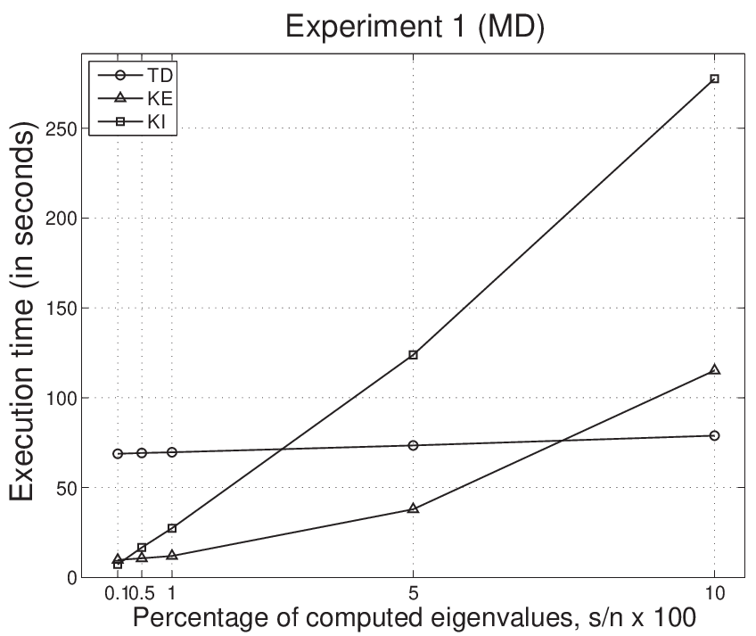
Figure 2 re-evaluates the performance of variants td, ke, and ki as a function of $s$ , now leveraging the implementation of these solvers using the kernels in the conventional+modern libraries. The results exhibit a rapid increase in the execution time of the variants based on the Krylov-subspace with the dimension of $s$ , due to the growth in the number of iterative steps, especially for ki.

6 Conclusions

We presented a performance study for the solution of generalized eigenproblems on multi-threaded architectures. The focus was on two different approaches: the reduction to tridiagonal form —either directly or in successive steps—, and the iterative solution through a Krylov method. In both cases, we first built the eigensolvers on top of conventional numerical libraries (BLAS, LAPACK, SBR, and ARPACK), and then compared with implementations that make use of modern multi-threaded libraries (libflame, PLASMA, MAGMA, and CUBLAS) as well as a few GPU kernels that we developed ourselves. As testbeds, we chose matrices arising in large-scale molecular dynamics and density functional theory; in both applications, only a portion of the lower part of the spectrum is of interest. The results are representative of the benefits that one should expect from GPUs and multi-threaded libraries; moreover, they indicate that in realistic applications, when only 3–5% of the spectrum is required, the Krylov-subspace solver is to be preferred.

References

[1] Jose I. Aliaga, Matthias Bollhöfer, Alberto F. Martín, and Enrique S. Quintana-Ortí. Exploiting thread-level parallelism in the iterative solution of sparse linear systems. Parallel Computing, 37(3):183–202, 2011.
[2] E. Anderson, Z. Bai, J. Demmel, J. E. Dongarra, J. DuCroz, A. Greenbaum, S. Hammarling, A. E. McKenney, S. Ostrouchov, and D. Sorensen. LAPACK Users’ Guide. SIAM, Philadelphia, 1992.
[3] ARPACK project home page. http://www.caam.rice.edu/software/ARPACK/.
[4] Rosa M. Badia, José R. Herrero, Jesús Labarta, Josep M. Pérez, Enrique S. Quintana-Ortí, and Gregorio Quintana-Ortí. Parallelizing dense and banded linear algebra libraries using SMPSs. Concurrency and Computation: Practice and Experience, 21(18):2438–2456, 2009.
[5] Sergio Barrachina, Maribel Castillo, Francisco D. Igual, Rafael Mayo, Enrique S. Quintana-Ortí, and Gregorio Quintana-Ortí. Exploiting the capabilities of modern GPUs for dense matrix computations. Concurrency and Computation: Practice and Experience, 21(18):2457–2477, 2009.
[6] P. Bientinesi, I. S. Dhillon, and R. van de Geijn. A parallel eigensolver for dense symmetric matrices based on multiple relatively robust representations. SIAM J. Sci. Comput., 27(1):43–66, 2005.
[7] Paolo Bientinesi, Francisco D. Igual, Daniel Kressner, Matthias Petschow, and Enrique S. Quintana-Ortí. Condensed forms for the symmetric eigenvalue problem on multi-threaded architectures. Concurrency and Computation: Practice and Experience, 23(7):694–707, 2011.
[8] C. H. Bischof, B. Lang, and X. Sun. Algorithm 807: The SBR Toolbox—software for successive band reduction. ACM Trans. Math. Soft., 26(4):602–616, 2000.
[9] S. Blügel, G. Bihlmayer, D. Wortmann, C. Friedrich, M. Heide, M. Lezaic, F. Freimuth, and M. Betzinger. The Jülich FLEUR project. http://www.flapw.de, 1987.
[10] Alfredo Buttari, Julien Langou, Jakub Kurzak, , and Jack Dongarra. A class of parallel tiled linear algebra algorithms for multicore architectures. Parallel Computing, 35(1):38–53, 2009.
[11] Q. Cui and I. Bahar. Normal Mode Analysis Theoretical and Applications to Biological and Chemical Systems. Mathematical & Computational Biology. Chapman & Hall/CRC, 2005.
[12] CULA project home page. http://www.culatools.com/.
[13] D. Davidović and E. S. Quintana-Ortí. Applying OOC techniques in the reduction to condensed form for very large symmetric eigenproblems on GPUs. In Proceedings of the 20th Euromicro Conference on Parallel, Distributed and Network based Processing – PDP 2012, pages 442–449, 2012.
[14] Inderjit S. Dhillon and Beresford N. Parlett. Multiple representations to compute orthogonal eigenvectors of symmetric tridiagonal matrices. Linear Algebra and its Applications, 387:1 – 28, 2004.
[15] FLAME project home page. http://www.cs.utexas.edu/users/flame/.
[16] L. Giraud, J. Langou, M. Rozloznik, and J. van den Eshof. Rounding error analysis of the classic Gram-Schmidt orthogonalization process. Numerische Mathematik, 101(1):87–100, 2005.
[17] Gene H. Golub and Charles F. Van Loan. Matrix Computations. The Johns Hopkins University Press, Baltimore, 3rd edition, 1996.
[18] J.R. Lopez-Blanco, J. I. Garzon, and P. Chacon. iMod: multipurpose normal mode analysis in internal coordinates. Bioinformatics, 2012. To appear.
[19] MAGMA project home page. http://icl.cs.utk.edu/magma/.
[20] NVIDIA Corporation. NVIDIA CUDA Compute Unified Device Architecture Programming Guide, 2.3.1 edition, August 2009.
[21] M. Petschow, E. Peise, and P. Bientinesi. High-performance solvers for large-scale dense eigensolvers. Technical Report AICES-2011/09-X, AICES, RWTH-Aachen, 2011.
[22] PLASMA project home page. http://icl.cs.utk.edu/plasma/.
[23] Gregorio Quintana-Ortí, Enrique S. Quintana-Ortí, Robert van de Geijn, Field Van Zee, and Ernie Chan. Programming matrix algorithms-by-blocks for thread-level parallelism. ACM Transactions on Mathematical Software, 36(3):14:1–14:26, 2009.
[24] L. Skjaerven, S.M. Hollup, and N. Reuter. Normal mode analysis for proteins. J. Mol. Struct., 898:42–48, 2009.
[25] F. Tama and C.L. Brooks. Symmetry, form, and shape: guiding principles for robustness in macromolecular machines.
[26] Vasily Volkov and James Demmel. LU, QR and Cholesky factorizations using vector capabilities of GPUs. Technical Report UCB/EECS-2008-49, EECS Department, University of California, Berkeley, May 2008.
[27] Field G. Van Zee. libflame: The Complete Reference. www.lulu.com, 2009.

Solving Dense Generalized Eigenproblems on Multi-threaded Architectures