Steady-state cracking in brittle substrates beneath adherent films: revisited

E. Matsinos^∗ Address: Centre for Applied Mathematics and Physics, Zurich University of Applied Sciences, Technikumstrasse 9, P.O. Box, CH-8401 Winterthur, Switzerland

Abstract

This is a technical note aiming at the re-examination of the phenomenon of the steady-state cracking in the two-layer system. The method of Suo and Hutchinson, as introduced in their $1989$ paper, is followed. Our solution is compared with the one appearing in that paper for the substrate-to-film thickness ratio $\lambda_{0}=10$ . We obtain results at three $\lambda_{0}<10$ values. Combined with the results for $\lambda_{0}=10$ , the new sets of values cover thickness ratios between $1$ and $10$ , sufficient for determining crack initiation and propagation in almost every relevant problem. We present our results in tables (and figures), thus facilitating their implementation and use.
PACS: 62.20.Mk; 81.40.Np

Keywords:

Steady-state cracking; two-layer system

^∗E-mail address: evangelos.matsinos@zhaw.ch

1 Introduction

The phenomenon of the steady-state cracking in the two-layer system was investigated in the work of Suo and Hutchinson [1] more than thirty years ago. In the present study, we will assume familiarity with the content of that paper; definitions for some of the quantities, which were introduced therein, will be given for reasons of clarity. Unless mentioned otherwise, the Suo-Hutchinson notation (of that paper) will be closely followed.

A two-layer system is produced when a block of material $1$ , typically a thin metallic plate or film, is attached to (e.g., glued or deposited upon) a block of material $2$ . In view of the interest in terms of application, we will assume that material $2$ is a semiconductor; by no means, should this be taken as a restriction of the method. Under the influence of external factors (e.g., via the application of mechanical force), a crack may appear and propagate at some depth in material $2$ . Steady-state cracking implies the propagation of the crack parallel to the interface of the two materials; this is one of the possible outcomes and, perhaps, the most interesting one in practical applications. Other possibilities include substrate cracking in the direction perpendicular to the interface, interface debonding, channelling, film buckling, etc. For details, the reader is addressed to Ref. [2].

The interest in the phenomenon of cracking is attributable to the production of thin slices of semiconductors (e.g., silicon); typical thicknesses span tens to a few hundreds of microns. At present, this technology offers the only available solution for large-scale production in case that the desirable thickness of the extracted slice exceeds a few tens of microns.

Despite that the theoretical background in Ref. [1] is independent of the specific technique used in the cracking, it was nonetheless developed for stresses which are mechanically induced, i.e., for crack initiation and propagation under the application of mechanical force on the sides of the two-layer system (e.g., see Fig. 2 of Ref. [1]). Another technique has gained ground in the recent years, namely, that of thermally-induced stress (e.g., see Refs. [2] and [3]), featuring the insertion of the two-layer system into an environment of temperature (far) below the one corresponding to the preparation (paste/deposition of material $1$ on material $2$ ). Given the difference of the coefficients of thermal expansion of the metal and of the semiconductor, the film bends first, thus inducing stress onto the substrate, which (depending on the conditions, materials, and thicknesses) may lose its cohesion and break. Finally, the metallic film tears off a layer of the semiconductor (which may be subsequently retrieved with further processing, e.g., via the use of a metal-etching solution [3]).

Irrespective of the technique employed in the cracking (i.e., mechanically- or thermally-induced stress, or a combination of the two), the basic phenomenon may be described by a simple model of effective longitudinal (mechanical) loads and moments [1], which are linked to the stress intensity factors $K_{I}$ and $K_{II}$ in the volume of material $2$ (see Eq. (6) of Ref. [1]). Suo and Hutchinson introduced a parameterisation (through their Eqs. (8)-(11)) in order to enable the evaluation of $K_{I}$ and $K_{II}$ in material $2$ from the effective mechanical load and moment; apart from the physical constants of the materials, introduced by their Eq. (9) is the angle $\omega$ , the only unknown in the evaluation. Having obtained $\omega$ as a function of the depth in material $2$ (for the materials being used), one may determine $K_{I}$ and $K_{II}$ in material $2$ and decide if (and where) a crack will be initiated and how it is expected to propagate. Evidently, crack initiation will occur at a position where the total stress exceeds the fracture toughness of the substrate $K_{Ic}$ (which, in silicon, is about $0.9$ MPa $\sqrt{\rm m}$ ). In case that $K_{II}=0$ in a path parallel to the interface of the two materials, the crack is expected to travel along that path [1]. By varying the external conditions (i.e., the mechanical forces and/or the temperature difference), material $1$ , its thickness, as well as the thickness of the silicon substrate, one may control the thickness of the peeled-off semiconductor slice (and the quality of the extraction, reflected in the variation of the thickness over the slice).

At this point, the reader might wonder why should the subject be revisited. There are a number of reasons calling for further results. The first and most important reason concerns the extraction of $\omega$ for more values of the substrate-to-film thickness ratio (hereafter denoted as $\lambda_{0}$ ); the two cases, which are fully documented in Ref. [1], i.e., $\lambda_{0}^{-1}=0$ and $0.10$ , are hardly sufficient when determining the stress intensity factors in the general case (i.e., at arbitrary $\lambda_{0}^{-1}$ ). (It must be noted that the $\omega$ values of [1] for the $\lambda_{0}^{-1}=0.05$ case are not useful, as the corresponding corrections for $\beta\neq 0$ have not been reported.) In the present paper, we plan to extract the $\omega$ values for $\lambda_{0}^{-1}=0.25$ , $0.50$ , and $1.00$ , i.e., for smaller substrate-to-film thickness ratios than those treated in Ref. [1]. We also plan to extract the $\omega$ values for $\lambda_{0}^{-1}=0.10$ and compare our results to those of Ref. [1].

Concerning the determination of the $\omega$ values at arbitrary $\lambda_{0}^{-1}\neq 0$ or $0.10$ , Suo and Hutchinson [1] wrote: ‘It is believed that $\omega$ is analytic in $\lambda_{0}^{-1}$ for large $\lambda_{0}$ , and therefore $\omega$ can be well approximated by linear interpolation in $\lambda_{0}^{-1}$ between $\lambda_{0}^{-1}=0$ and $0.10$ , where values of $\omega$ have been tabulated.’ Upon inspection, however, of the entries of their Tables $3$ - $5$ , one cannot but feel somewhat uneasy about that statement. Were it valid, one should be able to obtain the solution for $\lambda_{0}^{-1}=0.05$ (listed in their Table $4$ ) as average values of the corresponding entries of their Tables $3$ and $5$ . As a matter of fact, the solution of their Table $4$ systematically exceeds this average by anything up to $1.6^{0}$ , the average difference being equal to $0.66^{0}$ . Additionally, there are large curvature effects for $\lambda\gtrsim 3$ , the worst of which show up at $\alpha=0$ and $\lambda=6$ , where the three solutions are given as: $52.0$ , $51.0$ , and $46.8^{0}$ for $\lambda_{0}^{-1}=0$ , $0.05$ , and $0.10$ , respectively. For $9$ out of the $54$ cases in Tables $3$ - $5$ (for which a comparison is possible), monotony does not seem to hold at all; in this respect, the $\omega$ values at $\alpha=0.8$ are particularly problematic.

Regarding the corrections which must be applied (to the $\omega$ values) because of a non-zero $\beta$ , some numbers have appeared in Tables $1$ and $2$ of Ref. [1], yet in a form which makes the application of the correction difficult. The improvement we propose at this point is simple. We found that, for a given ( $\alpha$ , $\lambda_{0}$ , $\lambda$ ) combination, the assumption that the correction (defined as the $\omega$ value at $\beta\neq 0$ minus the one at $\beta=0$ ) scales with $\beta$ is a good approximation. We will therefore give these multiplicative factors for each ( $\alpha$ , $\lambda_{0}$ , $\lambda$ ) combination treated; the corrections may be easily obtained via a simple multiplication with the $\beta$ value. As the corrections for negative and positive $\beta$ values came out different, two sets of correction factors for each ( $\alpha$ , $\lambda_{0}$ , $\lambda$ ) combination will be given.

Last but not least, the present work serves one additional purpose. A detailed technical report on how to obtain the $\omega$ values will be surely useful in the future to anyone who has interest in studying further the phenomenon of cracking in the two-layer (perhaps, also in the three-layer) system. We find it surprising that, despite the fairly-broad use of the results of Ref. [1] (e.g., in finite-element calculations in Materials Science), no effort has been made in more than thirty years (to the best of the author’s knowledge) towards a further study of multi-layer systems within the framework set forth in that pioneering work.

2 Method

2.1 The Suo-Hutchinson model

The thickness of material $1$ is denoted by $h$ ; all relevant lengths in the problem will be expressed as multiples of $h$ . The thickness of material $2$ is denoted as $\lambda_{0}h$ . We will generally use the inverse of $\lambda_{0}$ in this paper; in this case, the solution for an infinitely-thick substrate corresponds to $\lambda_{0}^{-1}=0$ , for a substrate ten times thicker than the film to $\lambda_{0}^{-1}=0.10$ , and so on.

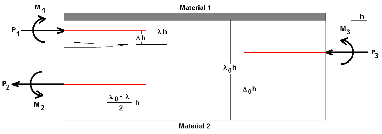
Shown in Fig. 1, is a crack propagating at depth $\lambda h$ inside the material $2$ (the depth is equal to $0$ at the interface of materials $1$ and $2$ ). Let us assume that the crack is propagating under the exertion of the longitudinal loads $P_{i}$ and moments $M_{i},i=1,2,3$ (both expressed ‘per unit of thickness’), applied to the two-layer system at the positions corresponding to the neutral axes. The positions of the neutral axes are obtained via the formulae

\Delta=\frac{\lambda^{2}+2\Sigma\lambda+\Sigma}{2(\lambda+\Sigma)}

(1)

and

\Delta_{0}=\frac{\lambda_{0}^{2}+2\Sigma\lambda_{0}+\Sigma}{2(\lambda_{0}+\Sigma)}\,,

(2)

where the quantity $\Sigma$ is the stiffness ratio of materials $1$ and $2$

\Sigma=\frac{1+\alpha}{1-\alpha}\,,

(3)

with

\alpha=\frac{\Gamma(\kappa_{2}+1)-(\kappa_{1}+1)}{\Gamma(\kappa_{2}+1)+(\kappa_{1}+1)}\,;

(4)

$\Gamma=\frac{\mu_{1}}{\mu_{2}}$ denotes the ratio of the shear moduli $\mu$ (the shear modulus is the ratio of the shear stress to the shear strain) of the two materials; $\kappa=3-4\nu$ for plane strain and $(3-\nu)/(1+\nu)$ for plane stress; finally, $\nu$ denotes Poisson’s ratio (the transverse-to-axial strain ratio when the material is stretched). The quantity $\alpha$ is one of the two parameters introduced by Dundurs [4] for the description of the mechanical properties of bimaterial systems; the second parameter is another combination of $\Gamma$ and of the $\kappa_{i}$ ’s

\beta=\frac{\Gamma(\kappa_{2}-1)-(\kappa_{1}-1)}{\Gamma(\kappa_{2}+1)+(\kappa_{1}+1)}\,.

(5)

It has been argued in the literature that $\beta$ reflects the oscillatory behaviour of the crack tip as the crack propagates in material $2$ . If materials $1$ and $2$ are equally stiff, then $\Sigma=1$ , in which case Eqs. (1,2) reduce to $\Delta=(\lambda+1)/2$ and $\Delta_{0}=(\lambda_{0}+1)/2$ ; therefore, in the trivial case of identical materials $1$ and $2$ , the neutral axes correspond, as expected, to the midpoints of the left (above the crack level) and right sides.

Suo and Hutchinson show (see Appendix A of Ref.[1]) that the phenomenon is adequately described on the basis of one effective longitudinal load $P$ and one moment $M$ . They come to this simplification after considering the two conditions for no net translation and rotation of the two-layer system (i.e., their Eqs. (3)), as well as the stress inside material $1$ before and after the crack tip; the effective quantities $P$ and $M$ may be obtained via the relations

P\equiv P_{1}-C_{1}P_{3}-C_{2}M_{3}/h

(6)

and

M\equiv M_{1}-C_{3}M_{3}\,,

(7)

with

C_{1}=A/A_{0}\,,

(8)

C_{2}=A[(\lambda_{0}-\Delta_{0})-(\lambda-\Delta)]/I_{0}\,,

(9)

and

C_{3}=I/I_{0}\,.

(10)

The expressions for the effective cross section $A$ and the moment of inertia (per unit length) $I$ may be found in Appendix A of that paper:

A=\lambda+\Sigma

(11)

and

I=\{\Sigma[3(\Delta-\lambda)^{2}-3(\Delta-\lambda)+1]+3\Delta\lambda(\Delta-\lambda)+\lambda^{3}\}/3\,.

(12)

Evidently,

A_{0}=\lambda_{0}+\Sigma

(13)

and

I_{0}=\{\Sigma[3(\Delta_{0}-\lambda_{0})^{2}-3(\Delta_{0}-\lambda_{0})+1]+3\Delta_{0}\lambda_{0}(\Delta_{0}-\lambda_{0})+\lambda_{0}^{3}\}/3\,.

(14)

Suo and Hutchinson subsequently proceed to associate the effective quantities $P$ and $M$ directly with the stress intensity factors $K_{I}$ and $K_{II}$ in the interior of material $2$ , proposing a relation (their Eq. (6)) reading as

K_{I}+iK_{II}=\frac{1}{\sqrt{2}}\Big(a\frac{P}{\sqrt{Uh}}+b\frac{M}{\sqrt{Vh^{3}}}\Big)\,,

(15)

where $a$ and $b$ , dimensionless complex quantities of unit modulus, depend on $\alpha$ , $\beta$ , $\lambda_{0}$ , and $\lambda$ ; the functions $U$ and $V$ have been given in their Appendix A.

U^{-1}=A^{-1}+\frac{1}{\lambda_{0}-\lambda}+\frac{12[\Delta+(\lambda_{0}-\lambda)/2]^{2}}{(\lambda_{0}-\lambda)^{3}}

(16)

and

V^{-1}=I^{-1}+\frac{12}{(\lambda_{0}-\lambda)^{3}}\,.

(17)

The formalism is completed after putting $a$ and $b$ in the forms

a=e^{i\omega}

(18)

and

b=-ie^{i(\omega+\gamma)}\,,

(19)

where the angle $\gamma$ may be obtained (according to the third of their equations appearing under (A $8$ )) by using the formula

\gamma=\sin^{-1}\Big\{\frac{12\sqrt{UV}[\Delta+(\lambda_{0}-\lambda)/2]}{(\lambda_{0}-\lambda)^{3}}\Big\}\,.

(20)

Obviously, the only quantity which must be known in order that the stress intensity factors $K_{I}$ and $K_{II}$ be determined is the angle $\omega$ , which should be considered a function of $\alpha$ , $\beta$ , $\lambda_{0}$ , and $\lambda$ . After having set the $\lambda$ -dependence of $\omega$ for the specific ( $\alpha$ , $\beta$ , $\lambda_{0}$ ) combination, one may directly obtain the stress intensity factors in the entire volume of the semiconductor, and assess if (and where) a crack will be initiated and how it is expected to propagate. We will deal with the determination of the $\omega$ values in the following section.

2.2 Determination of the $\omega$ values

The extraction of the angle $\omega$ for each ( $\alpha$ , $\beta$ , $\lambda_{0}$ , $\lambda$ ) combination is a rather involved issue; it is recommended that the interested reader consult Appendices B and C of Ref. [1] for the details. Herein, we intend only to draw attention to a number of relevant issues. The integral equation, which is to be solved (i.e., Eq. (B $11$ ) of [1]), reads as

\int_{-1}^{1}\frac{\bar{A}(t)}{u-t}dt+\int_{-1}^{1}\frac{F_{1}(\zeta)A(t)+[1+t+F_{2}(\zeta)]\bar{A}(t)}{(1+t)^{2}}dt=0\,,

(21)

where $\bar{A}(t)$ denotes the complex conjugate of $A(t)$ . The quantities $u$ and $t$ are real numbers satisfying $-1<u,t<1$ ; $\zeta=\frac{2(u-t)}{(u+1)(t+1)}$ . The complex functions $F_{1,2}(t)$ are defined in Appendix C of Ref. [1]. The complex function $A(t)$ is expanded in terms of the Chebyshev polynomials of the first kind $T_{k}(t)$ :

A(t)=\Big(\frac{1-t}{2}\Big)^{-1/2}\big[B(-\infty)+(1+t)\sum_{k=1}^{N}a_{k}T_{k-1}(t)\big]\,,

(22)

where $B(-\infty)$ is a complex constant with known imaginary part (see the first of Eqs. (B $7$ ) of Ref.[1]) and $a_{k}$ are complex coefficients, the real and imaginary parts of which must be determined. Without loss of generality, the real part of $a_{N}$ may be set to $0$ , after which there are $2N$ unknowns in the problem (i.e., $2N-1$ numbers associated with the coefficients $a_{k}$ and $\Re[B(-\infty)]$ ). The integral equation (21) is solved on $N$ $u_{i}$ points, chosen to be the $N$ Gauss-Legendre points in $[-1,1]$ , and the decomposition of the set into real and imaginary parts yields $2N$ equations, i.e., as many as unknowns in the problem. The set of equations may be written in a compact form as

\sum_{k=1}^{N}[a_{k}I_{1}(u,k)+\bar{a}_{k}I_{2}(u,k)]+\Re[B(-\infty)]I_{3}(u)=I_{4}(u)\,.

(23)

As only $I_{1}(u,k)$ has been explicitly given in Ref. [1], we will now list all expressions;

I_{1}(u,k)=\int_{-1}^{1}\frac{F_{1}(\zeta)}{1+t}\Big(\frac{1-t}{2}\Big)^{-1/2}T_{k-1}(t)dt\,,

(24)

	$\displaystyle I_{2}(u,k)=$	$\displaystyle\int_{-1}^{1}\frac{1}{u-t}\Big(\frac{1-t}{2}\Big)^{-1/2}(1+t)T_{k-1}(t)dt+$
		$\displaystyle\int_{-1}^{1}\frac{1+t+F_{2}(\zeta)}{1+t}\Big(\frac{1-t}{2}\Big)^{-1/2}T_{k-1}(t)dt\,,$		(25)

	$\displaystyle I_{3}(u)=$	$\displaystyle\int_{-1}^{1}\frac{1}{u-t}\Big(\frac{1-t}{2}\Big)^{-1/2}dt+\int_{-1}^{1}\frac{F_{1}(\zeta)}{(1+t)^{2}}\Big(\frac{1-t}{2}\Big)^{-1/2}dt+$
		$\displaystyle\int_{-1}^{1}\frac{1+t+F_{2}(\zeta)}{(1+t)^{2}}\Big(\frac{1-t}{2}\Big)^{-1/2}dt\,,$		(26)

and

$\displaystyle I_{4}(u)=-i\Im[B(-\infty)]\Big\{-$	$\displaystyle\int_{-1}^{1}\frac{1}{u-t}\Big(\frac{1-t}{2}\Big)^{-1/2}dt+$
	$\displaystyle\int_{-1}^{1}\frac{F_{1}(\zeta)}{(1+t)^{2}}\Big(\frac{1-t}{2}\Big)^{-1/2}dt-$
	$\displaystyle\int_{-1}^{1}\frac{1+t+F_{2}(\zeta)}{(1+t)^{2}}\Big(\frac{1-t}{2}\Big)^{-1/2}dt\Big\}\,.$	(27)

Given the asymptotic behaviour of the functions $F_{1,2}(t)$ (see Eqs. (B $3$ ) of [1]), all integrands behave well as $t\to-1$ (equivalently, $\zeta\to\infty$ ) and all integrals exist. The quantities $I_{2,3,4}$ contain terms in which Cauchy principal values must be determined (i.e., the integrands involving the inverse of $u-t$ ). The method of Longman [5] has been used to estimate the contribution in $I_{2}(u,k)$ ; the value of the integral, appearing in $I_{3,4}$ , may be obtained analytically.

We now touch upon one important point, namely the choice of the number $N$ of Chebyshev polynomials to be used in the expansion of $A(t)$ . In Ref.[1], it is noted that the results had been obtained ‘with $N$ between $10$ and $15$ .’ We have varied $N$ between $6$ and $16$ (with a step of $2$ ), but we have not been able to observe true convergence in the extracted $\omega$ values; the $\omega$ values (in most cases) come out close (within a range of $2^{0}$ ), yet the characteristic trend, resembling an approach to an asymptotic value, was rarely observed. Concerning the point of whether true convergence had been observed in the cases reported in Ref. [1], the text is of little help. Suo and Hutchinson write at the end of their Appendix B: ‘The consistency check was satisfied to better than $0.1\%$ . It is believed that the accuracy in $\omega$ is comparable.’ One may speculate on the meaning of these statements. If by ‘consistency check’ the authors imply the fulfillment of the convergence criterion (i.e., the $\omega$ values for successive $N$ runs differ less than $0.1\%$ of their average), the fact that two successive $\omega$ values happen to come out ‘close enough’ should not be taken as evidence of true convergence; for instance, we observed (several times) that the $\omega$ values for $N=10$ and $12$ came out close, but at least one of the subsequent values (i.e., those corresponding to $N=14$ or $16$ ) was distant, yet not distant enough to be considered an outlier. Although Suo and Hutchinson might have imposed additional constraints (e.g., on the behaviour of the coefficients $a_{k}$ ), which have not been mentioned in their paper, it seems difficult to obtain a solution in this problem, accurate down to the $0.1\%$ level. We have not been able to resolve this issue with the authors of Ref. [1]. Lacking the exact details on how the results of Ref. [1] were obtained at this point (and whether true convergence had been observed in the cases reported), we will follow another strategy in determining the final $\omega$ value (and its associated uncertainty) in each ( $\alpha$ , $\beta$ , $\lambda_{0}$ , $\lambda$ ) combination; this is the subject of the next section.

After the solution for the coefficients $a_{k}$ and for $\Re[B(-\infty)]$ is obtained, the $\omega$ value is extracted using the relation

\omega=-\tan^{-1}\Big\{\frac{\Im[B(-\infty)+2\sum_{k=1}^{N}a_{k}]}{\Re[B(-\infty)+2\sum_{k=1}^{N}a_{k}]}\Big\}-\gamma\,,

(28)

the angle $\gamma$ being taken from Eq. (20).

2.3 Some technical issues

2.3.1 Extraction of the $\omega$ values

As six $N$ values have been used in Eq. (22), six $\omega$ values are extracted in each ( $\alpha$ , $\beta$ , $\lambda_{0}$ , $\lambda$ ) combination. In a perfect world, it is expected that these values show trends of convergence, i.e., of ‘approaching’ the asymptotic value, defined as the limit when $N\to\infty$ . As mentioned earlier, we have not been able to observe traces of such a behaviour in the majority of the cases examined. Presumably, this failure is due to the combination of two effects: a) imprecision in the evaluation of the integrals entering the terms $I_{i}$ and b) ‘noise’ introduced by the inversion of large matrices for the extraction of the unknowns $a_{k}$ and $\Re[B(-\infty)]$ (when $N=16$ , a $32\times 32$ matrix must be inverted).

In the absence of signs of convergence in the series of the extracted values of $\omega$ , we have decided to determine one average $\omega$ value, as well as the associated uncertainty per case, i.e., per ( $\alpha$ , $\beta$ , $\lambda_{0}$ , $\lambda$ ) combination, and further process the resulting data. It is not easy, however, to produce meaningful averages and uncertainties from only six data points, especially so in the presence of outliers. Consequently, the first step in the evaluation of $\omega$ must involve the employment of an efficient algorithm for outlier rejection. A few outlier-detection algorithms have been tested. The first successful results were obtained with Grubbs’s outlier test [6, 7]; although the test checks the input data for the presence of one single outlier, it may enable, if iterated, the exclusion of several deviant points. In a number of cases, however, the process of applying Grubbs’s test iteratively terminated at the first step, declaring no outliers, though the visual inspection of the data easily (and clearly) identified two outliers. (This is a known problem for Grubbs’s outlier test.) As a result, we decided to apply a more recent algorithm, namely, Rosner’s generalised ESD (Extreme Studentised Deviate) test [8]. In this algorithm, a set of $N_{k}$ data points is tested for the presence of exactly $1$ , $2$ , …, $N_{a}$ outliers, where $N_{a}$ is a user-defined integer satisfying the condition $N_{a}<N_{k}$ (in fact, it does not make much sense to perform the test with $N_{a}$ exceeding $N_{k}/2$ ); the advantage of Rosner’s test is that the ‘optimal’ number of outliers is extracted from the input data set.

The maximal number of outliers $N_{a}$ was set to $3$ in the analysis. Three significance levels were used: $0.20$ , $0.10$ , and $0.05$ ; large values of the significance level result in the detection of many outliers, small ones leave outliers in the data. The results for the three significance levels were always compared prior to making decisions. At each significance level, Rosner’s test is (in our case) performed for exactly one, two, and three outliers in each input data set. At each of these three steps, the set of candidate outliers is accepted or rejected on the basis of the comparison of the score value of the test statistic with a critical value, which depends on the number of ‘good’ points (those points which do not belong to the set of candidate outliers) and on the significance level. Of course, if no score value exceeds the critical one at any step, the input data set contains no outliers.

One example of extracted $\omega$ values, obtained for ( $\alpha$ , $\beta$ , $\lambda_{0}^{-1}$ , $\lambda$ ) $=$ ( $-0.60$ , $0$ , $0.25$ , $1.0$ ), is shown in Fig. 2. We will now examine what actually happens if the $\omega$ values, shown in this figure, are submitted to Rosner’s test. Let us fix the confidence level to $0.20$ . The assumption that the data contains exactly one outlier is first tested. The highest $\omega$ value in the sample (which is the most deviant data point) is tested first; its score value is equal to $1.6462$ , whereas the critical score value is (for the confidence level used and for a six-element set) $1.7289$ . As a result, the point may not be considered an outlier (at this step). (Grubbs’s test would have terminated at this point.) The sample is then tested for the presence of exactly two outliers (the two candidates now being the previous candidate outlier and the most distant value after the first candidate outlier is removed from the data, i.e., the lowest $\omega$ value). The score value for the second potential outlier is equal to $1.7535$ , whereas the critical score value (for the confidence level used and for a five-element set) is $1.6016$ . Therefore, the result of the test for two outliers is affirmative, the largest and smallest values in the data set having been established as true outliers. The sample is then tested for exactly three outliers (the two already-established outliers and the most deviant of the remaining values); tested at this step is the value obtained for $N=6$ . The score value for the third potential outlier is equal to $1.3680$ , whereas the critical score value (for the confidence level used and for a four-element set) is $1.4250$ . The final conclusion is that there are only two outliers in the data (the highest number of established outliers in the $N_{a}$ steps of the test). The results of this test for the other two significance levels agree with the presence of only two outliers in the data (identical to those established at the $0.20$ significance level). The two outliers were removed from the input data and the average value and the associated uncertainty (the standard error of the means) were estimated from the remaining measurements and stored as final result of the processing for the specific ( $\alpha$ , $\beta$ , $\lambda_{0}$ , $\lambda$ ) combination.

Described in the example of Fig. 2 is one clear-cut case, as the results obtained at the three significance levels agree. In many cases, however, the numbers of outliers for the three significance levels come out different. In order to avoid glitches in the application of the algorithm, we decided to set up an interactive procedure and also visually inspect the data, parallel to the application of the algorithm. Special attention was paid when the $\omega$ values came out close (e.g., not more than a few tenths of one degree apart); in that case, the test was not performed and all data were accepted in the evaluation of the $\omega$ average and the accompanying uncertainty. Given the smallness of the initial sample, potentially problematic are the cases with one-sided (i.e., lying on the same side of the average) outliers; one may easily obtain an erroneous average. There is less risk in case that the two outliers lie on either side of the average (only the uncertainty depends on the treatment, i.e., on the exclusion or inclusion of both values); fortunately, most cases with two outliers fall in this last category.

The $\omega$ values at $\lambda_{0}\leq 4$ contain very few outliers. On the contrary, the $\lambda_{0}=10$ data contain many values which seem to be ‘out of place’, especially so in the small- $\lambda$ region; additionally, the $N=6$ and $16$ solutions contain values which fluctuate to the extent that the rejection of the corresponding sets is called for more often than not. To overcome the problem of submitting obvious outliers to the outlier-detection algorithm, we have decided to first visually inspect the tables of the data obtained at fixed values of $\alpha$ , $\beta$ , and $\lambda_{0}$ ; in these tables of $\omega$ values, the rows indicate different $\lambda$ values, whereas the columns different $N$ values. After the removal of the obvious outliers in each table, there are three options one may follow.

•

Perform an overall fit to all surviving data (assuming constant uncertainties) and present the fitted values as the optimal solution. In this case, it is recommended that a robust fit be made to the data.
•

Fit the data in columns (i.e., variable $\lambda$ , fixed $N$ ) and ‘fill in’ the values at the places which contained the (removed) outliers. One may then search for outliers in the $N$ direction (i.e., for fixed $\lambda$ ), with the application of Rosner’s test, as described earlier. The estimated average values and accompanying uncertainties may be submitted to the final fit, for the creation of a smooth solution at the given ( $\alpha$ , $\beta$ , $\lambda_{0}$ ) combination.
•

The third case combines the two aforementioned options and, because of this, it may be more reliable. In order to obtain an impression of the overall trend of the data, one starts with a (robust) fit to all values. One then applies the second option, using the obtained trend as guideline whenever a decision must be made when performing Rosner’s test (e.g., in case of different numbers of outliers for the three significance levels).

Despite the fact that we have followed the second option in the analysis, we have nevertheless compared, at the final step, our solution with the results of the robust fit to the data.

A few comments concerning the form of the functions, which have been used in the fits, are due. Given the absence of theoretical guideline regarding the $\lambda$ -dependence of the angle $\omega$ , our objective is simply to choose forms which may efficiently achieve the data description. To this end, maximal freedom must be rendered to the data by choosing forms with many adjustable parameters; in such cases, the rule of thumb usually is that the introduction of one additional parameter should not bring noticeable improvement of the data description (there exist accurate tests, via the comparison of the $p$ -values of the corresponding fits). To enable a judgement on the quality of the reproduction of the data, the original data will also be shown in almost all the figures in Section 3. We will now comment on the empirical forms we have chosen.

•

$\alpha<-0.05$ . It is evident from the inspection of the $\omega$ values that a curve, which is capable of describing data with negative curvature, must be fitted to the data. We have tested a few forms and finally decided to make use of the sum of an exponential and a $\Gamma$ function (six parameters in total).
•

$-0.05\leq\alpha\leq 0.05$ . There is some curvature in the $\alpha=-0.05$ data in the small- $\lambda$ region. The data at $\alpha=0.05$ do not show significant curvature. In both cases, a cubic fit to the logarithm of the $\omega$ values was found adequate.
•

$\alpha>0.05$ . This was the most demanding case as the data show a sharp increase for decreasing $\lambda$ . The fits were performed on the basis of a six-degree polynomial to the extracted $\omega$ values. A few other functions were also tested, but yielded inferior results.

We will now comment on a number of additional technical points. The integrations yielding the terms $I_{i}$ (given in Eqs. (24)-(27)) were performed by using the trapezoidal rule (with the tolerance level set to $10^{-6}$ ). Other methods were tried (e.g., Romberg’s integration method), but were found slow and did not yield more accurate results. The stability (in the series of the extracted $\omega$ values) increases substantially, if the integrations relating to $I_{1}(u,k)$ and $I_{2}(u,k)$ are performed within the roots of the Chebyshev polynomials. The values of the functions $Q_{1,2}(\zeta)$ and $R_{1,2}(\zeta)$ (see Eqs. (C13) of [1]) were obtained by using the (fast) Gauss-Legendre quadrature with $256$ nodes ( $1,024$ nodes were also used without improving the results). We also applied the Hurwitz-Zweifel method [9, 10], but could not obtain accurate enough results in the problem. It is essential in the evaluation to set the regions of importance of the functions $F_{1,2}(\zeta)$ properly. Adaptive integration methods should (in principle) find fertile ground for application in this subject, yet (despite the effort) we have not been able to set up such a scheme in a direct way. Instead, we have implemented an indirect way of incorporating adaptivity, by setting the step in the tabulation of $F_{1,2}(\zeta)$ in such a way as to account for the importance (largeness) of the corresponding values of (each of) these functions. Hence, the very detailed (high-resolution) step (of $10^{-4}$ in $\zeta$ ) was used in the important regions (defined as those regions where the value of the corresponding function exceeds $1\%$ of the global maximum), whereas the low-resolution step (of $10^{-2}$ in $\zeta$ ) was used below that level. Contributions, falling below the (arbitrary) $10^{-6}$ level irrevocably, were not pursued further (thus, the tails of the integrands make no contributions to the evaluation of the terms $I_{i}$ of Eqs. (24)-(27)).

2.3.2 Optimisation

For the purpose of fitting, the standard MINUIT package [11] of the CERN library was used; to be precise, we have used the C++ version of the library [12]. Extensive information on this software package may be obtained from the internet [13]. The latest release of the code is available from [14]. Version $5.28.00$ of Minuit2 (i.e., the current version at the moment we set out on this program) was incorporated in the analysis framework. Each optimisation was achieved on the basis of the (robust) SIMPLEX-MINIMIZE-MIGRAD chain. All fits terminated successfully.

The optimisation of the data description was achieved via the minimisation of a standard $\chi^{2}$ function; $\chi^{2}$ is defined as the sum of the squares of the normalised residuals over all input data points. For each data point, the normalised residual is defined as the difference between the raw (experimental) and fitted (theoretical) values, divided by the uncertainty of the ‘measurement’. The fitted values are obtained on the basis of a parametric model, for fixed values of the model parameters; evidently, $\chi^{2}$ is a function of the parameter vector. Technically, the optimisation terminates when, by the elaborate variation of the parameter vector, the global minimum of the minimisation function is reached (more precisely, when the expected distance to the global minimum falls below a user-defined threshold, expressed via the setting of the accuracy level in the optimisation).

For the robust fits, mentioned in Section 2.3.1, another minimisation function was chosen, namely one which is defined as the sum of the terms $\ln(1+r_{i}^{2})$ , where $r_{i}$ is the normalised residual of the $i$ -th data point. Compared to the standard $\chi^{2}$ function, this form is significantly less sensitive to the presence of outliers.

2.3.3 $\beta$ correction

Unlike Ref. [1], we do not intend to give values of the angle $\omega$ (as a function of $\lambda$ ) in some $\beta\neq 0$ cases at fixed values of $\alpha$ . Instead, we will give optimal values for the factor $c(\alpha,\lambda_{0}^{-1};\lambda)$ defined as

c(\alpha,\lambda_{0}^{-1};\lambda)=\frac{\omega(\alpha,\beta,\lambda_{0}^{-1};\lambda)-\omega(\alpha,0,\lambda_{0}^{-1};\lambda)}{\beta}\,,

(29)

thus enabling the straightforward evaluation of $\omega(\alpha,\beta,\lambda_{0}^{-1};\lambda)$ from the tabulated values of $\omega(\alpha,0,\lambda_{0}^{-1};\lambda)$ . As it turned out that the constants $c(\alpha,\lambda_{0}^{-1};\lambda)$ were different for $\beta<0$ and $\beta>0$ , two factors per ( $\alpha$ , $\lambda_{0}$ , $\lambda$ ) case will be given. The creation of these values also involves a step in which fitting empirical functions to the data, identified as the right-hand side of Eq. (29), was performed using (again) the MINUIT library.

3 Results

We will now present our results for a number of values of $\lambda\leq\lambda_{0}/2$ . The values of $\lambda_{0}^{-1}$ treated in the present study are: $0.10$ , $0.25$ , $0.50$ , and $1.00$ . We will compare our results for $\lambda_{0}^{-1}=0.10$ with those obtained in Ref. [1] (which reports no results for $\lambda_{0}^{-1}>0.10$ ). Given the occasional instability at $\alpha=0$ (especially at small values of $\lambda$ ¹¹ 1 The increasing instability as $\lambda$ approaches $0$ may have been the reason that Suo and Hutchinson [1] give no solution below $\lambda=1.0$ in the $\lambda_{0}^{-1}=0.05$ case.), the values of the parameter $\alpha$ used were: $\pm 0.6$ , $\pm 0.4$ , $\pm 0.2$ , and $\pm 0.05$ . For the first three cases and for $\alpha=0$ , Ref. [1] has reported results; additionally, Ref. [1] has extracted the $\omega$ values at $\alpha=\pm 0.8$ ²² 2 For plane strain and silicon substrate, the $\alpha$ values when using Al, Cu, Ag, and Ti films are: $-0.37$ , $-0.09$ , $-0.30$ , and $-0.13$ , i.e., well within the $\alpha$ interval of this work.). The values of the parameter $\beta$ are subjected to the condition $\frac{\alpha-1}{4}\leq\beta\leq\frac{\alpha+1}{4}$ [1]; two values close to the upper and lower limits, as well as the reference value of $\beta=0$ , were used.

It must be mentioned that the extraction of the $\omega$ values does not occur without effort. For instance, the $\lambda_{0}^{-1}=0.10$ case will involve $624$ combinations of the parameter values, each combination (run) requiring anything between $30$ and $90$ minutes on a fairly-fast computer, i.e., an overall time load of no less than about three weeks. The $\omega$ values were produced with a dedicated C/C++-based $64$ -bit application, developed within the Microsoft Visual Studio $9.0$ framework and run on an Intel^© Core ${}^{\rm TM}2$ Duo Processor T $9600$ at $2.80$ GHz.

We will first give our results for $\lambda_{0}^{-1}=0.10$ . Our solution for $\omega$ as a function of $\lambda$ is given in Table 1 (for the eight $\alpha$ values used herein). The comparison of the results of this work with the Suo-Hutchinson values ³³ 3 By plotting the Suo-Hutchinson data (versus $\lambda$ ), one cannot fail noticing that the values must have been subjected to some smoothing; they seem too ‘good’ to have been obtained directly. We have not found comments on this issue in Ref. [1]. may be found in Figs. 3-10. We observe that the two sets of data agree well, save for a few values in the small- $\lambda$ region. Small differences are also observed around $\lambda=1.0$ for $\alpha<0$ , but die off rapidly with increasing $\lambda$ .

For $\alpha=-0.60$ , our fitted solution slightly exceeds the values reported in Ref.[1] in the region $0.3\leq\lambda\leq 1.0$ , by about $0.40^{0}$ . For $\alpha=-0.40$ , the Suo-Hutchinson solution exceeds ours at small $\lambda$ , by about $0.9^{0}$ at $\lambda=0.1$ ; the two solutions cross each other between $\lambda=0.2$ and $0.3$ , after which our solution is larger by no more than about $0.45^{0}$ , until the difference drops below $0.1^{0}$ above $\lambda=1.0$ . A similar trend may be observed for $\alpha=-0.20$ . For $\alpha>0$ , the shapes of the two solutions are slightly different in the small- $\lambda$ region, our values exceeding those of Suo and Hutchinson by a few tenths of one degree. Evidently, the most serious discrepancy occurs at $\alpha=0.6$ ; all $\omega$ values between $\lambda=0.1$ and $0.6$ strongly disagree, the largest discrepancy ( $2.4^{0}$ ) occurring at $\lambda=0.1$ . The differences fall below $0.1^{0}$ above $\lambda=0.7$ . Despite the effort, we have not been able to pin down the source of this discrepancy, which appears to be persistent irrespective of the treatment of the data and method of outlier detection and removal.

We have compared our solution with the one obtained on the basis of the robust fit to the data after the removal of only the obvious outliers. Given that the difference to the Suo-Hutchinson values is significant only when $\alpha=0.6$ , we will report only in that case. The result of the robust fit to the data ( $93$ data points in total) gives slightly different values for $\lambda=0.1$ , $0.2$ , and $0.3$ ; the values obtained are: $64.66$ , $61.78$ , and $59.41^{0}$ , respectively; above $\lambda=0.3$ , the differences between the two solutions remain below $0.1^{0}$ . Evidently, the robust-fit solution confirms the results of the elaborate analysis and thorough outlier rejection as described in Section 2.3.

The two sets of the $\beta$ -correction factors $c(\alpha,\lambda_{0}^{-1};\lambda)$ , defined in Eq. (29), for the $\lambda_{0}^{-1}=0.10$ case are given in Tables 2 and 3. Both factors show peaks below $\lambda=1.0$ . For negative values of $\beta$ , the maximal correction is around $3.40^{0}$ at $\alpha=-0.6$ , dropping down to $1.21^{0}$ at $\alpha=0.6$ ; the minimal correction remains above $-0.37^{0}$ . For positive values of $\beta$ the corrections lie between $-2.92$ and $2.37^{0}$ . Of course, the limits given in this paragraph are linked to the domain of the $\alpha$ values used in the present work.

The detailed comparison with the results of Suo and Hutchinson, wherever it was possible to compare the two $\beta$ corrections, is given in Table 4. We observe that the differences between the two solutions do not exceed a few tenths of one degree (actually, between $-0.32$ and $0.30^{0}$ ), with an average value of $0.02^{0}$ and a root-mean-square of $0.11^{0}$ .

Our results for the angle $\omega$ for $\lambda_{0}^{-1}=0.25$ , $0.50$ , and $1.00$ are to be found in Tables 5, 7, and 9, respectively. The corresponding correction factors $c(\alpha,\lambda_{0}^{-1};\lambda)$ , defined in Eq. (29), are listed in Tables 6, 8, and 10. Concerning these cases, the only interesting remark is that the extracted $\omega$ values showed less fluctuation than in the $\lambda_{0}^{-1}=0.10$ case. All data have been obtained by applying the process outlined in Section 2.3.1 and have been subjected to smoothing as described in Section 2.3.2. In schematic form, the data (along with the fitted curves) are displayed in Figs. 11-13; the uncertainties have been omitted. It is interesting to notice that the $\beta$ corrections may become important close to the interface of the two materials for $\alpha>0$ , more important than they seem to be in the $\lambda_{0}^{-1}=0.10$ case.

4 Conclusions

Our aim in this work has been to re-address the subject of steady-state cracking, originally investigated by Suo and Hutchinson [1] more than thirty years ago. One of the reasons calling for further investigation is the extraction of solutions for values of the substrate-to-film thickness ratio smaller than $10$ , which was the lowest value treated in the Suo-Hutchinson paper. To this end, we produced the solutions for the ratio values of $4$ , $2$ , and $1$ . Our solutions may be used as ‘anchor points’ in the evaluation of the quantity $\omega$ (introduced in Ref. [1], to link the external mechanical loads and moments with the stress intensity factors) in the general problem of arbitrary thickness ratio.

We have also obtained the solution in one of the two cases treated in Ref. [1], namely at the substrate-to-film thickness ratio of $10$ . We have concluded that the two sets of $\omega$ values agree well, save for distances close to the interface of the two materials (small $\lambda$ values), where a significant difference (of $2.4^{0}$ ) has been found on one occasion.

We have not been able to observe true convergence in the series of the extracted $\omega$ values when increasing the dimensionality of the problem, i.e., the number of Chebyshev polynomials used in Eq. (22). In the absence of convergence, we have decided to apply an algorithm for the detection of outliers, estimate the average values (and accompanying uncertainties) of the surviving data points, and fit simple forms to the resulting (‘clean’) data. We present our results in tabular form, thus enabling their easy implementation.

One of the important contributions of the present work is the introduction of a well-ordered scheme for the application of the $\beta$ correction. Essential, in this respect, was the observation that this correction scales with $\beta$ , yet differently for positive and negative $\beta$ values. To facilitate the application of this correction, we have given the relevant multiplicative factors in tabular form.

The author acknowledges helpful discussions with Peter Biller.

References

[1] Z. Suo and J.W. Hutchinson, ‘Steady-state cracking in brittle substrates beneath adherent films’, International Journal of Solids and Structures 25 (1989) 1337.
[2] J.W. Hutchinson and Z. Suo, ‘Mixed Mode Cracking in Layered Materials’, Advances in Applied Mechanics 29 (1992) 63.
[3] F. Dross et al., ‘Stress-induced large-area lift-off of crystalline Si films’, Applied Physics A 89 (2007) 149.
[4] J. Dundurs, ‘Elastic interaction of dislocations with inhomogeneities’, ed. T. Mura, Mathematical Theory of Dislocations, ASME, New York (1969) 70.
[5] I.M. Longman, ‘On the numerical evaluation of Cauchy principal values of integrals’, Mathematical Tables and Other Aids to Computation 12 (1958) 205.
[6] F.E. Grubbs, ‘Procedures for Detecting Outlying Observations in Samples’, Technometrics 11 (1969) 1.
[7] W. Stefansky, ‘Rejecting Outliers in Factorial Designs’, Technometrics 14 (1972) 469.
[8] B. Rosner, ‘Percentage Points for a Generalized ESD Many-Outlier Procedure’, Technometrics 25 (1983) 165.
[9] H. Hurwitz and P.F. Zweifel, ‘Numerical Quadrature of Fourier Transform Integrals’, Mathematical Tables and Other Aids to Computation 55 (1956) 140.
[10] H. Hurwitz, R.A. Pfeiffer, and P.F. Zweifel, ‘Numerical Quadrature of Fourier Transform Integrals II’, Mathematical Tables and Other Aids to Computation 66 (1959) 87.
[11] F. James, ‘MINUIT - Function Minimization and Error Analysis’, CERN Program Library Long Writeup D506.
[12] F. James and M. Winkler, ‘MINUIT User’s Guide’, 2004.
[13] http://project-mathlibs.web.cern.ch/project-mathlibs/sw/Minuit2/html/index.html
[14] http://seal.web.cern.ch/seal/snapshot/work-packages/mathlibs/minuit/

Table 1:

The values of the angle $\omega$ (in degrees) for $\lambda_{0}^{-1}=0.10$ and $\beta=0$ .

$\lambda\downarrow$ , $\alpha\rightarrow$	$-0.60$	$-0.40$	$-0.20$	$-0.05$	$0.05$	$0.20$	$0.40$	$0.60$
$0.1$	$44.66$	$46.12$	$49.33$	$51.28$	$52.36$	$55.43$	$58.83$	$64.81$
$0.2$	$48.57$	$49.08$	$50.57$	$51.39$	$52.30$	$54.55$	$57.26$	$61.91$
$0.3$	$50.57$	$50.65$	$51.25$	$51.48$	$52.24$	$53.83$	$55.94$	$59.51$
$0.4$	$51.73$	$51.57$	$51.67$	$51.57$	$52.17$	$53.24$	$54.83$	$57.54$
$0.5$	$52.42$	$52.14$	$51.94$	$51.64$	$52.11$	$52.76$	$53.91$	$55.92$
$0.6$	$52.83$	$52.49$	$52.12$	$51.70$	$52.05$	$52.37$	$53.14$	$54.61$
$0.7$	$53.06$	$52.70$	$52.23$	$51.75$	$52.00$	$52.06$	$52.51$	$53.55$
$0.8$	$53.18$	$52.81$	$52.31$	$51.79$	$51.94$	$51.81$	$51.99$	$52.68$
$0.9$	$53.22$	$52.86$	$52.35$	$51.82$	$51.88$	$51.61$	$51.57$	$51.98$
$1.0$	$53.21$	$52.87$	$52.37$	$51.84$	$51.82$	$51.44$	$51.22$	$51.41$
$1.1$	$53.16$	$52.84$	$52.37$	$51.85$	$51.76$	$51.31$	$50.93$	$50.94$
$1.2$	$53.10$	$52.80$	$52.35$	$51.85$	$51.70$	$51.20$	$50.69$	$50.55$
$1.3$	$53.01$	$52.74$	$52.33$	$51.85$	$51.65$	$51.11$	$50.50$	$50.22$
$1.4$	$52.92$	$52.67$	$52.30$	$51.83$	$51.59$	$51.03$	$50.33$	$49.93$
$1.5$	$52.83$	$52.60$	$52.26$	$51.81$	$51.53$	$50.95$	$50.18$	$49.68$
$1.6$	$52.73$	$52.53$	$52.21$	$51.78$	$51.47$	$50.88$	$50.06$	$49.46$
$1.7$	$52.64$	$52.45$	$52.16$	$51.74$	$51.41$	$50.80$	$49.94$	$49.26$
$1.8$	$52.54$	$52.37$	$52.10$	$51.70$	$51.35$	$50.73$	$49.84$	$49.07$
$1.9$	$52.45$	$52.29$	$52.04$	$51.64$	$51.29$	$50.66$	$49.74$	$48.90$
$2.0$	$52.36$	$52.21$	$51.98$	$51.59$	$51.22$	$50.58$	$49.65$	$48.74$
$2.5$	$51.93$	$51.80$	$51.60$	$51.21$	$50.89$	$50.18$	$49.21$	$48.11$
$3.0$	$51.49$	$51.36$	$51.13$	$50.73$	$50.51$	$49.76$	$48.84$	$47.78$
$3.5$	$51.00$	$50.86$	$50.60$	$50.18$	$50.08$	$49.39$	$48.54$	$47.63$
$4.0$	$50.41$	$50.27$	$50.00$	$49.60$	$49.58$	$49.03$	$48.27$	$47.32$
$4.5$	$49.70$	$49.58$	$49.35$	$49.04$	$48.99$	$48.57$	$47.83$	$46.65$
$5.0$	$48.88$	$48.79$	$48.66$	$48.52$	$48.31$	$47.96$	$47.03$	$46.40$

Table 2:

The $\beta$ -correction factors $c(\alpha,\lambda_{0}^{-1}=0.10;\lambda)$ (in degrees), defined in Eq. (29), for $\beta<0$ .

$\lambda\downarrow$ , $\alpha\rightarrow$	$-0.60$	$-0.40$	$-0.20$	$-0.05$	$0.05$	$0.20$	$0.40$	$0.60$
$0.10$	$-2.83$	$-2.38$	$-1.59$	$-0.83$	$-0.25$	$0.71$	$2.13$	$3.72$
$0.20$	$-7.63$	$-8.33$	$-8.59$	$-8.58$	$-8.50$	$-8.27$	$-7.81$	$-7.20$
$0.30$	$-8.49$	$-9.56$	$-10.21$	$-10.52$	$-10.66$	$-10.78$	$-10.79$	$-10.66$
$0.40$	$-8.27$	$-9.48$	$-10.32$	$-10.80$	$-11.06$	$-11.37$	$-11.67$	$-11.86$
$0.50$	$-7.69$	$-8.93$	$-9.86$	$-10.43$	$-10.77$	$-11.21$	$-11.70$	$-12.10$
$0.60$	$-6.99$	$-8.21$	$-9.19$	$-9.81$	$-10.19$	$-10.71$	$-11.33$	$-11.88$
$0.70$	$-6.28$	$-7.46$	$-8.44$	$-9.09$	$-9.50$	$-10.07$	$-10.77$	$-11.43$
$0.80$	$-5.60$	$-6.73$	$-7.70$	$-8.36$	$-8.78$	$-9.38$	$-10.14$	$-10.87$
$0.90$	$-4.98$	$-6.05$	$-6.99$	$-7.65$	$-8.07$	$-8.69$	$-9.48$	$-10.25$
$1.00$	$-4.42$	$-5.43$	$-6.34$	$-6.99$	$-7.41$	$-8.02$	$-8.83$	$-9.62$
$1.10$	$-3.93$	$-4.87$	$-5.74$	$-6.37$	$-6.78$	$-7.39$	$-8.20$	$-9.01$
$1.20$	$-3.49$	$-4.37$	$-5.20$	$-5.81$	$-6.21$	$-6.81$	$-7.60$	$-8.41$
$1.30$	$-3.10$	$-3.93$	$-4.71$	$-5.30$	$-5.68$	$-6.26$	$-7.04$	$-7.83$
$1.40$	$-2.76$	$-3.53$	$-4.28$	$-4.83$	$-5.20$	$-5.76$	$-6.52$	$-7.29$
$1.50$	$-2.46$	$-3.18$	$-3.88$	$-4.41$	$-4.77$	$-5.30$	$-6.03$	$-6.78$
$1.60$	$-2.20$	$-2.87$	$-3.53$	$-4.03$	$-4.37$	$-4.88$	$-5.58$	$-6.29$
$1.70$	$-1.97$	$-2.59$	$-3.21$	$-3.69$	$-4.01$	$-4.49$	$-5.16$	$-5.84$
$1.80$	$-1.77$	$-2.35$	$-2.93$	$-3.37$	$-3.68$	$-4.14$	$-4.77$	$-5.42$
$1.90$	$-1.59$	$-2.13$	$-2.67$	$-3.09$	$-3.38$	$-3.81$	$-4.41$	$-5.03$
$2.00$	$-1.44$	$-1.94$	$-2.44$	$-2.84$	$-3.10$	$-3.51$	$-4.08$	$-4.66$
$2.50$	$-0.89$	$-1.23$	$-1.58$	$-1.86$	$-2.05$	$-2.34$	$-2.75$	$-3.17$
$3.00$	$-0.58$	$-0.81$	$-1.05$	$-1.23$	$-1.36$	$-1.56$	$-1.84$	$-2.13$
$3.50$	$-0.38$	$-0.54$	$-0.70$	$-0.82$	$-0.91$	$-1.04$	$-1.22$	$-1.42$
$4.00$	$-0.26$	$-0.36$	$-0.46$	$-0.54$	$-0.60$	$-0.69$	$-0.81$	$-0.93$
$4.50$	$-0.17$	$-0.24$	$-0.31$	$-0.36$	$-0.39$	$-0.45$	$-0.53$	$-0.61$
$5.00$	$-0.12$	$-0.16$	$-0.20$	$-0.23$	$-0.26$	$-0.29$	$-0.34$	$-0.39$

Table 3:

The $\beta$ -correction factors $c(\alpha,\lambda_{0}^{-1}=0.10;\lambda)$ (in degrees), defined in Eq. (29), for $\beta>0$ .

$\lambda\downarrow$ , $\alpha\rightarrow$	$-0.60$	$-0.40$	$-0.20$	$-0.05$	$0.05$	$0.20$	$0.40$	$0.60$
$0.10$	$-6.00$	$-4.01$	$-2.03$	$-0.54$	$0.45$	$1.94$	$3.93$	$5.92$
$0.20$	$-8.99$	$-7.57$	$-6.14$	$-5.07$	$-4.36$	$-3.29$	$-1.87$	$-0.45$
$0.30$	$-9.45$	$-8.47$	$-7.49$	$-6.75$	$-6.26$	$-5.53$	$-4.55$	$-3.57$
$0.40$	$-9.18$	$-8.55$	$-7.91$	$-7.44$	$-7.12$	$-6.65$	$-6.01$	$-5.38$
$0.50$	$-8.64$	$-8.27$	$-7.91$	$-7.63$	$-7.45$	$-7.17$	$-6.81$	$-6.44$
$0.60$	$-7.99$	$-7.83$	$-7.67$	$-7.55$	$-7.47$	$-7.35$	$-7.19$	$-7.02$
$0.70$	$-7.32$	$-7.31$	$-7.30$	$-7.30$	$-7.30$	$-7.29$	$-7.29$	$-7.28$
$0.80$	$-6.66$	$-6.76$	$-6.87$	$-6.95$	$-7.01$	$-7.09$	$-7.19$	$-7.30$
$0.90$	$-6.03$	$-6.22$	$-6.41$	$-6.55$	$-6.64$	$-6.79$	$-6.98$	$-7.17$
$1.00$	$-5.44$	$-5.68$	$-5.93$	$-6.12$	$-6.24$	$-6.42$	$-6.67$	$-6.92$
$1.10$	$-4.89$	$-5.18$	$-5.46$	$-5.67$	$-5.81$	$-6.03$	$-6.31$	$-6.60$
$1.20$	$-4.39$	$-4.70$	$-5.00$	$-5.23$	$-5.39$	$-5.61$	$-5.92$	$-6.23$
$1.30$	$-3.94$	$-4.25$	$-4.57$	$-4.80$	$-4.96$	$-5.20$	$-5.51$	$-5.83$
$1.40$	$-3.52$	$-3.84$	$-4.16$	$-4.39$	$-4.55$	$-4.79$	$-5.11$	$-5.42$
$1.50$	$-3.15$	$-3.46$	$-3.77$	$-4.00$	$-4.16$	$-4.39$	$-4.70$	$-5.02$
$1.60$	$-2.81$	$-3.11$	$-3.41$	$-3.64$	$-3.79$	$-4.01$	$-4.32$	$-4.62$
$1.70$	$-2.51$	$-2.79$	$-3.08$	$-3.30$	$-3.44$	$-3.66$	$-3.94$	$-4.23$
$1.80$	$-2.23$	$-2.51$	$-2.78$	$-2.98$	$-3.12$	$-3.32$	$-3.59$	$-3.87$
$1.90$	$-1.99$	$-2.24$	$-2.50$	$-2.69$	$-2.82$	$-3.01$	$-3.26$	$-3.52$
$2.00$	$-1.77$	$-2.01$	$-2.24$	$-2.42$	$-2.54$	$-2.72$	$-2.96$	$-3.19$
$2.50$	$-0.98$	$-1.13$	$-1.29$	$-1.40$	$-1.48$	$-1.59$	$-1.75$	$-1.90$
$3.00$	$-0.53$	$-0.63$	$-0.72$	$-0.79$	$-0.83$	$-0.90$	$-0.99$	$-1.09$
$3.50$	$-0.29$	$-0.34$	$-0.39$	$-0.43$	$-0.46$	$-0.50$	$-0.55$	$-0.60$
$4.00$	$-0.15$	$-0.18$	$-0.21$	$-0.23$	$-0.25$	$-0.27$	$-0.30$	$-0.33$
$4.50$	$-0.08$	$-0.10$	$-0.11$	$-0.12$	$-0.13$	$-0.14$	$-0.16$	$-0.18$
$5.00$	$-0.04$	$-0.05$	$-0.06$	$-0.07$	$-0.07$	$-0.08$	$-0.08$	$-0.09$

Table 4:

The comparison of the $\beta$ corrections between the Suo-Hutchinson solution [1] and those obtained in this work. The first three columns correspond to the values of the parameters $\alpha$ , $\beta$ , and $\lambda$ , for which results have been reported in Ref. [1]. (As our solution does not include the $\alpha$ values of $\pm 0.8$ , no comparison can be made in this case.) The next column ( $\tilde{\omega}_{0}$ ) contains the Suo-Hutchinson solution at the specific $\alpha$ and $\lambda$ values, at $\beta=0$ . The adjacent column ( $\tilde{\omega}$ ) contains their solution for the $\beta$ value given in the second column. The difference of the two aforementioned angles is shown next; this is the Suo-Hutchinson correction due to the non-zero $\beta$ value. We subsequently give our $\beta$ -correction factor $c$ , taken directly from Tables 2 and 3, depending on the sign of $\beta$ . Our correction (shown next) has been obtained by multiplying $\beta$ and the factor $c$ . The last column contains the difference between the two $\beta$ corrections (i.e., our result minus the corresponding Suo-Hutchinson value). All angles (as well as the multiplicative factors $c$ ) are given in degrees. The numerical results of this table have been rounded to two decimal places.

$\alpha$	$\beta$	$\lambda$	$\tilde{\omega}_{0}$	$\tilde{\omega}$	$\tilde{\omega}-\tilde{\omega_{0}}$	$c$	$\omega-\omega_{0}$	$\delta$
$-0.60$	$-0.40$	$0.5$	$52.00$	$55.40$	$3.40$	$-7.69$	$3.08$	$-0.32$
$-0.60$	$-0.40$	$1.0$	$52.90$	$54.80$	$1.90$	$-4.42$	$1.77$	$-0.13$
$-0.60$	$-0.40$	$1.5$	$52.70$	$53.80$	$1.10$	$-2.46$	$0.98$	$-0.12$
$-0.60$	$-0.40$	$2.0$	$52.30$	$52.90$	$0.60$	$-1.44$	$0.58$	$-0.02$
$-0.60$	$-0.40$	$3.0$	$51.40$	$51.70$	$0.30$	$-0.58$	$0.23$	$-0.07$
$-0.60$	$-0.40$	$4.0$	$50.40$	$50.40$	$0.00$	$-0.26$	$0.10$	$0.10$
$-0.60$	$-0.40$	$5.0$	$49.00$	$49.10$	$0.10$	$-0.12$	$0.05$	$-0.05$
$-0.40$	$-0.30$	$0.5$	$51.70$	$54.50$	$2.80$	$-8.93$	$2.68$	$-0.12$
$-0.40$	$-0.30$	$1.0$	$52.70$	$54.40$	$1.70$	$-5.43$	$1.63$	$-0.07$
$-0.40$	$-0.30$	$1.5$	$52.55$	$53.60$	$1.05$	$-3.18$	$0.95$	$-0.10$
$-0.40$	$-0.30$	$2.0$	$52.20$	$52.80$	$0.60$	$-1.94$	$0.58$	$-0.02$
$-0.40$	$-0.30$	$3.0$	$51.40$	$51.60$	$0.20$	$-0.81$	$0.24$	$0.04$
$-0.40$	$-0.30$	$4.0$	$50.30$	$50.40$	$0.10$	$-0.36$	$0.11$	$0.01$
$-0.40$	$-0.30$	$5.0$	$48.90$	$49.00$	$0.10$	$-0.16$	$0.05$	$-0.05$
$-0.40$	$0.10$	$0.5$	$51.70$	$51.00$	$-0.70$	$-8.27$	$-0.83$	$-0.13$
$-0.40$	$0.10$	$1.0$	$52.70$	$52.20$	$-0.50$	$-5.68$	$-0.57$	$-0.07$
$-0.40$	$0.10$	$1.5$	$52.55$	$52.30$	$-0.25$	$-3.46$	$-0.35$	$-0.10$
$-0.40$	$0.10$	$2.0$	$52.20$	$52.00$	$-0.20$	$-2.01$	$-0.20$	$0.00$
$-0.40$	$0.10$	$3.0$	$51.40$	$51.30$	$-0.10$	$-0.63$	$-0.06$	$0.04$
$-0.40$	$0.10$	$4.0$	$50.30$	$50.20$	$-0.10$	$-0.18$	$-0.02$	$0.08$
$-0.40$	$0.10$	$5.0$	$48.90$	$48.90$	$0.00$	$-0.05$	$-0.01$	$-0.01$

Table 4 continued

$\alpha$	$\beta$	$\lambda$	$\tilde{\omega}_{0}$	$\tilde{\omega}$	$\tilde{\omega}-\tilde{\omega_{0}}$	$c$	$\omega-\omega_{0}$	$\delta$
$-0.20$	$-0.30$	$0.5$	$51.70$	$54.70$	$3.00$	$-9.86$	$2.96$	$-0.04$
$-0.20$	$-0.30$	$1.0$	$52.30$	$54.30$	$2.00$	$-6.34$	$1.90$	$-0.10$
$-0.20$	$-0.30$	$1.5$	$52.15$	$53.40$	$1.25$	$-3.88$	$1.16$	$-0.09$
$-0.20$	$-0.30$	$2.0$	$51.90$	$52.70$	$0.80$	$-2.44$	$0.73$	$-0.07$
$-0.20$	$-0.30$	$3.0$	$51.10$	$51.50$	$0.40$	$-1.05$	$0.31$	$-0.09$
$-0.20$	$-0.30$	$4.0$	$50.00$	$50.20$	$0.20$	$-0.46$	$0.14$	$-0.06$
$-0.20$	$-0.30$	$5.0$	$48.80$	$48.90$	$0.10$	$-0.20$	$0.06$	$-0.04$
$-0.20$	$0.10$	$0.5$	$51.70$	$50.90$	$-0.80$	$-7.91$	$-0.79$	$0.01$
$-0.20$	$0.10$	$1.0$	$52.30$	$51.80$	$-0.50$	$-5.93$	$-0.59$	$-0.09$
$-0.20$	$0.10$	$1.5$	$52.15$	$51.90$	$-0.25$	$-3.77$	$-0.38$	$-0.13$
$-0.20$	$0.10$	$2.0$	$51.90$	$51.70$	$-0.20$	$-2.24$	$-0.22$	$-0.02$
$-0.20$	$0.10$	$3.0$	$51.10$	$51.00$	$-0.10$	$-0.72$	$-0.07$	$0.03$
$-0.20$	$0.10$	$4.0$	$50.00$	$50.00$	$0.00$	$-0.21$	$-0.02$	$-0.02$
$-0.20$	$0.10$	$5.0$	$48.80$	$48.70$	$-0.10$	$-0.06$	$-0.01$	$0.09$
$0.20$	$-0.20$	$0.5$	$52.50$	$54.50$	$2.00$	$-11.21$	$2.24$	$0.24$
$0.20$	$-0.20$	$1.0$	$51.40$	$53.00$	$1.60$	$-8.02$	$1.60$	$0.00$
$0.20$	$-0.20$	$1.5$	$51.05$	$52.00$	$0.95$	$-5.30$	$1.06$	$0.11$
$0.20$	$-0.20$	$2.0$	$50.70$	$51.40$	$0.70$	$-3.51$	$0.70$	$0.00$
$0.20$	$-0.20$	$3.0$	$50.00$	$50.40$	$0.40$	$-1.56$	$0.31$	$-0.09$
$0.20$	$-0.20$	$4.0$	$49.20$	$49.30$	$0.10$	$-0.69$	$0.14$	$0.04$
$0.20$	$-0.20$	$5.0$	$48.00$	$48.10$	$0.10$	$-0.29$	$0.06$	$-0.04$
$0.20$	$0.20$	$0.5$	$52.50$	$50.90$	$-1.60$	$-7.17$	$-1.43$	$0.17$
$0.20$	$0.20$	$1.0$	$51.40$	$50.20$	$-1.20$	$-6.42$	$-1.28$	$-0.08$
$0.20$	$0.20$	$1.5$	$51.05$	$50.10$	$-0.95$	$-4.39$	$-0.88$	$0.07$
$0.20$	$0.20$	$2.0$	$50.70$	$50.10$	$-0.60$	$-2.72$	$-0.54$	$0.06$
$0.20$	$0.20$	$3.0$	$50.00$	$49.70$	$-0.30$	$-0.90$	$-0.18$	$0.12$
$0.20$	$0.20$	$4.0$	$49.20$	$49.00$	$-0.20$	$-0.27$	$-0.05$	$0.15$
$0.20$	$0.20$	$5.0$	$48.00$	$48.00$	$0.00$	$-0.08$	$-0.02$	$-0.02$

Table 4 continued

$\alpha$	$\beta$	$\lambda$	$\tilde{\omega}_{0}$	$\tilde{\omega}$	$\tilde{\omega}-\tilde{\omega_{0}}$	$c$	$\omega-\omega_{0}$	$\delta$
$0.40$	$-0.10$	$0.5$	$53.50$	$54.50$	$1.00$	$-11.70$	$1.17$	$0.17$
$0.40$	$-0.10$	$1.0$	$51.20$	$52.00$	$0.80$	$-8.83$	$0.88$	$0.08$
$0.40$	$-0.10$	$1.5$	$50.25$	$50.80$	$0.55$	$-6.03$	$0.60$	$0.05$
$0.40$	$-0.10$	$2.0$	$49.80$	$50.20$	$0.40$	$-4.08$	$0.41$	$0.01$
$0.40$	$-0.10$	$3.0$	$49.10$	$49.30$	$0.20$	$-1.84$	$0.18$	$-0.02$
$0.40$	$-0.10$	$4.0$	$48.40$	$48.50$	$0.10$	$-0.81$	$0.08$	$-0.02$
$0.40$	$-0.10$	$5.0$	$47.40$	$47.50$	$0.10$	$-0.34$	$0.03$	$-0.07$
$0.40$	$0.30$	$0.5$	$53.50$	$51.40$	$-2.10$	$-6.81$	$-2.04$	$0.06$
$0.40$	$0.30$	$1.0$	$51.20$	$49.20$	$-2.00$	$-6.67$	$-2.00$	$0.00$
$0.40$	$0.30$	$1.5$	$50.25$	$48.80$	$-1.45$	$-4.70$	$-1.41$	$0.04$
$0.40$	$0.30$	$2.0$	$49.80$	$48.80$	$-1.00$	$-2.96$	$-0.89$	$0.11$
$0.40$	$0.30$	$3.0$	$49.10$	$48.60$	$-0.50$	$-0.99$	$-0.30$	$0.20$
$0.40$	$0.30$	$4.0$	$48.40$	$48.10$	$-0.30$	$-0.30$	$-0.09$	$0.21$
$0.40$	$0.30$	$5.0$	$47.40$	$47.20$	$-0.20$	$-0.08$	$-0.03$	$0.17$
$0.60$	$-0.10$	$0.5$	$55.40$	$56.40$	$1.00$	$-12.10$	$1.21$	$0.21$
$0.60$	$-0.10$	$1.0$	$51.40$	$52.30$	$0.90$	$-9.62$	$0.96$	$0.06$
$0.60$	$-0.10$	$1.5$	$49.65$	$50.30$	$0.65$	$-6.78$	$0.68$	$0.03$
$0.60$	$-0.10$	$2.0$	$48.80$	$49.20$	$0.40$	$-4.66$	$0.47$	$0.07$
$0.60$	$-0.10$	$3.0$	$47.90$	$48.20$	$0.30$	$-2.13$	$0.21$	$-0.09$
$0.60$	$-0.10$	$4.0$	$47.30$	$47.40$	$0.10$	$-0.93$	$0.09$	$-0.01$
$0.60$	$-0.10$	$5.0$	$46.50$	$46.60$	$0.10$	$-0.39$	$0.04$	$-0.06$
$0.60$	$0.30$	$0.5$	$55.40$	$53.50$	$-1.90$	$-6.44$	$-1.93$	$-0.03$
$0.60$	$0.30$	$1.0$	$51.40$	$49.30$	$-2.10$	$-6.92$	$-2.08$	$0.02$
$0.60$	$0.30$	$1.5$	$49.65$	$48.00$	$-1.65$	$-5.02$	$-1.50$	$0.15$
$0.60$	$0.30$	$2.0$	$48.80$	$47.60$	$-1.20$	$-3.19$	$-0.96$	$0.24$
$0.60$	$0.30$	$3.0$	$47.90$	$47.30$	$-0.60$	$-1.09$	$-0.33$	$0.27$
$0.60$	$0.30$	$4.0$	$47.30$	$46.90$	$-0.40$	$-0.33$	$-0.10$	$0.30$
$0.60$	$0.30$	$5.0$	$46.50$	$46.30$	$-0.20$	$-0.09$	$-0.03$	$0.17$

Table 5:

The fitted values of the angle $\omega$ (in degrees) for $\lambda_{0}^{-1}=0.25$ and $\beta=0$ .

$\lambda\downarrow$ , $\alpha\rightarrow$	$-0.60$	$-0.40$	$-0.20$	$-0.05$	$0.05$	$0.20$	$0.40$	$0.60$
$0.1$	$44.94$	$46.03$	$48.83$	$51.47$	$52.65$	$54.63$	$58.03$	$61.45$
$0.2$	$48.34$	$48.63$	$49.92$	$51.38$	$52.30$	$53.62$	$56.10$	$58.90$
$0.3$	$50.11$	$49.98$	$50.51$	$51.28$	$51.98$	$52.78$	$54.55$	$56.82$
$0.4$	$51.11$	$50.74$	$50.84$	$51.17$	$51.68$	$52.09$	$53.31$	$55.13$
$0.5$	$51.66$	$51.16$	$51.01$	$51.06$	$51.40$	$51.52$	$52.33$	$53.77$
$0.6$	$51.93$	$51.37$	$51.07$	$50.94$	$51.13$	$51.06$	$51.55$	$52.66$
$0.7$	$52.02$	$51.45$	$51.07$	$50.81$	$50.88$	$50.68$	$50.93$	$51.75$
$0.8$	$51.99$	$51.43$	$51.01$	$50.67$	$50.63$	$50.36$	$50.42$	$50.99$
$0.9$	$51.87$	$51.35$	$50.90$	$50.52$	$50.39$	$50.08$	$49.98$	$50.34$
$1.0$	$51.69$	$51.23$	$50.76$	$50.35$	$50.16$	$49.82$	$49.60$	$49.77$
$1.1$	$51.47$	$51.07$	$50.60$	$50.16$	$49.93$	$49.57$	$49.25$	$49.25$
$1.2$	$51.22$	$50.88$	$50.41$	$49.96$	$49.69$	$49.32$	$48.91$	$48.77$
$1.3$	$50.95$	$50.67$	$50.19$	$49.74$	$49.46$	$49.05$	$48.57$	$48.33$
$1.4$	$50.67$	$50.44$	$49.96$	$49.50$	$49.21$	$48.77$	$48.23$	$47.92$
$1.5$	$50.37$	$50.19$	$49.70$	$49.23$	$48.95$	$48.47$	$47.89$	$47.53$
$1.6$	$50.07$	$49.93$	$49.43$	$48.94$	$48.69$	$48.16$	$47.54$	$47.17$
$1.7$	$49.77$	$49.65$	$49.13$	$48.63$	$48.41$	$47.84$	$47.21$	$46.84$
$1.8$	$49.46$	$49.35$	$48.82$	$48.29$	$48.11$	$47.53$	$46.87$	$46.51$
$1.9$	$49.15$	$49.04$	$48.49$	$47.92$	$47.79$	$47.24$	$46.54$	$46.18$
$2.0$	$48.84$	$48.72$	$48.14$	$47.53$	$47.45$	$46.99$	$46.20$	$45.78$

Table 6:

The $\beta$ -correction factors $c(\alpha,\lambda_{0}^{-1}=0.25;\lambda)$ (in degrees), defined in Eq. (29); upper part: values for $\beta<0$ , lower part: values for $\beta>0$ .

$\lambda\downarrow$ , $\alpha\rightarrow$	$-0.60$	$-0.40$	$-0.20$	$-0.05$	$0.05$	$0.20$	$0.40$	$0.60$
$0.10$	$-4.11$	$-2.87$	$-1.05$	$0.61$	$1.84$	$3.83$	$6.75$	$9.94$
$0.20$	$-7.75$	$-7.54$	$-6.72$	$-5.81$	$-5.09$	$-3.86$	$-1.97$	$0.16$
$0.30$	$-8.29$	$-8.50$	$-8.17$	$-7.66$	$-7.23$	$-6.44$	$-5.18$	$-3.71$
$0.40$	$-7.97$	$-8.40$	$-8.37$	$-8.12$	$-7.87$	$-7.39$	$-6.58$	$-5.59$
$0.50$	$-7.34$	$-7.89$	$-8.05$	$-7.99$	$-7.88$	$-7.62$	$-7.14$	$-6.52$
$0.60$	$-6.61$	$-7.23$	$-7.52$	$-7.59$	$-7.58$	$-7.49$	$-7.25$	$-6.91$
$0.70$	$-5.87$	$-6.52$	$-6.90$	$-7.06$	$-7.12$	$-7.15$	$-7.11$	$-6.97$
$0.80$	$-5.17$	$-5.82$	$-6.25$	$-6.48$	$-6.59$	$-6.72$	$-6.81$	$-6.84$
$0.90$	$-4.52$	$-5.15$	$-5.62$	$-5.89$	$-6.04$	$-6.23$	$-6.44$	$-6.59$
$1.00$	$-3.93$	$-4.54$	$-5.02$	$-5.31$	$-5.49$	$-5.73$	$-6.01$	$-6.25$
$1.10$	$-3.39$	$-3.98$	$-4.46$	$-4.77$	$-4.96$	$-5.24$	$-5.57$	$-5.88$
$1.20$	$-2.92$	$-3.47$	$-3.94$	$-4.26$	$-4.47$	$-4.76$	$-5.13$	$-5.48$
$1.30$	$-2.50$	$-3.02$	$-3.47$	$-3.80$	$-4.00$	$-4.30$	$-4.69$	$-5.08$
$1.40$	$-2.13$	$-2.61$	$-3.05$	$-3.37$	$-3.57$	$-3.88$	$-4.28$	$-4.68$
$1.50$	$-1.81$	$-2.26$	$-2.67$	$-2.98$	$-3.18$	$-3.48$	$-3.88$	$-4.29$
$1.60$	$-1.53$	$-1.94$	$-2.34$	$-2.63$	$-2.82$	$-3.12$	$-3.52$	$-3.92$
$1.70$	$-1.29$	$-1.67$	$-2.04$	$-2.31$	$-2.50$	$-2.79$	$-3.17$	$-3.57$
$1.80$	$-1.08$	$-1.42$	$-1.77$	$-2.03$	$-2.21$	$-2.48$	$-2.86$	$-3.24$
$1.90$	$-0.90$	$-1.21$	$-1.53$	$-1.78$	$-1.95$	$-2.21$	$-2.56$	$-2.93$
$2.00$	$-0.75$	$-1.03$	$-1.32$	$-1.56$	$-1.72$	$-1.96$	$-2.30$	$-2.65$
$0.10$	$-1.02$	$0.09$	$2.13$	$4.24$	$5.91$	$8.82$	$13.43$	$18.84$
$0.20$	$-4.38$	$-4.91$	$-4.57$	$-3.78$	$-3.00$	$-1.47$	$1.23$	$4.66$
$0.30$	$-4.97$	$-5.93$	$-6.13$	$-5.80$	$-5.36$	$-4.38$	$-2.49$	$0.04$
$0.40$	$-4.88$	$-5.98$	$-6.41$	$-6.32$	$-6.06$	$-5.41$	$-4.04$	$-2.10$
$0.50$	$-4.58$	$-5.71$	$-6.25$	$-6.31$	$-6.18$	$-5.76$	$-4.76$	$-3.29$
$0.60$	$-4.22$	$-5.32$	$-5.92$	$-6.08$	$-6.04$	$-5.79$	$-5.09$	$-3.99$
$0.70$	$-3.83$	$-4.88$	$-5.52$	$-5.74$	$-5.77$	$-5.65$	$-5.18$	$-4.37$

Table 6 continued

$\lambda\downarrow$ , $\alpha\rightarrow$	$-0.60$	$-0.40$	$-0.20$	$-0.05$	$0.05$	$0.20$	$0.40$	$0.60$
$0.80$	$-3.45$	$-4.44$	$-5.08$	$-5.34$	$-5.42$	$-5.40$	$-5.11$	$-4.54$
$0.90$	$-3.08$	$-4.00$	$-4.62$	$-4.91$	$-5.02$	$-5.07$	$-4.92$	$-4.54$
$1.00$	$-2.73$	$-3.58$	$-4.17$	$-4.47$	$-4.60$	$-4.70$	$-4.65$	$-4.41$
$1.10$	$-2.41$	$-3.18$	$-3.73$	$-4.03$	$-4.17$	$-4.30$	$-4.33$	$-4.20$
$1.20$	$-2.12$	$-2.80$	$-3.32$	$-3.60$	$-3.75$	$-3.90$	$-3.98$	$-3.92$
$1.30$	$-1.84$	$-2.46$	$-2.93$	$-3.20$	$-3.34$	$-3.50$	$-3.61$	$-3.61$
$1.40$	$-1.60$	$-2.14$	$-2.57$	$-2.81$	$-2.95$	$-3.11$	$-3.24$	$-3.28$
$1.50$	$-1.38$	$-1.86$	$-2.23$	$-2.46$	$-2.59$	$-2.74$	$-2.88$	$-2.94$
$1.60$	$-1.19$	$-1.60$	$-1.94$	$-2.14$	$-2.26$	$-2.40$	$-2.54$	$-2.62$
$1.70$	$-1.01$	$-1.37$	$-1.67$	$-1.85$	$-1.96$	$-2.09$	$-2.22$	$-2.31$
$1.80$	$-0.86$	$-1.17$	$-1.43$	$-1.59$	$-1.69$	$-1.81$	$-1.93$	$-2.02$
$1.90$	$-0.73$	$-1.00$	$-1.22$	$-1.36$	$-1.45$	$-1.55$	$-1.67$	$-1.75$
$2.00$	$-0.62$	$-0.85$	$-1.04$	$-1.16$	$-1.23$	$-1.33$	$-1.44$	$-1.51$

Table 7:

The values of the angle $\omega$ (in degrees) for $\lambda_{0}^{-1}=0.50$ and $\beta=0$ .

$\lambda\downarrow$ , $\alpha\rightarrow$	$-0.60$	$-0.40$	$-0.20$	$-0.05$	$0.05$	$0.20$	$0.40$	$0.60$
$0.1$	$44.52$	$46.04$	$48.23$	$50.10$	$51.31$	$53.10$	$56.01$	$58.89$
$0.2$	$47.83$	$48.09$	$48.92$	$50.01$	$50.77$	$52.00$	$53.86$	$56.17$
$0.3$	$49.30$	$48.99$	$49.18$	$49.80$	$50.24$	$51.04$	$52.31$	$54.22$
$0.4$	$49.94$	$49.36$	$49.20$	$49.49$	$49.69$	$50.17$	$51.10$	$52.62$
$0.5$	$50.10$	$49.41$	$49.05$	$49.09$	$49.14$	$49.38$	$50.06$	$51.19$
$0.6$	$49.98$	$49.26$	$48.79$	$48.63$	$48.58$	$48.63$	$49.08$	$49.88$
$0.7$	$49.68$	$48.96$	$48.44$	$48.12$	$48.00$	$47.92$	$48.12$	$48.68$
$0.8$	$49.26$	$48.54$	$48.01$	$47.58$	$47.41$	$47.24$	$47.22$	$47.59$
$0.9$	$48.75$	$48.02$	$47.53$	$47.03$	$46.81$	$46.56$	$46.40$	$46.61$
$1.0$	$48.19$	$47.41$	$46.99$	$46.48$	$46.19$	$45.89$	$45.69$	$45.80$

Table 8:

The $\beta$ -correction factors $c(\alpha,\lambda_{0}^{-1}=0.50;\lambda)$ (in degrees), defined in Eq. (29); upper part: values for $\beta<0$ , lower part: values for $\beta>0$ .

$\lambda\downarrow$ , $\alpha\rightarrow$	$-0.60$	$-0.40$	$-0.20$	$-0.05$	$0.05$	$0.20$	$0.40$	$0.60$
$0.10$	$-1.43$	$-0.31$	$1.43$	$3.08$	$4.32$	$6.39$	$9.51$	$13.02$
$0.20$	$-5.28$	$-5.26$	$-4.50$	$-3.53$	$-2.73$	$-1.29$	$1.02$	$3.74$
$0.30$	$-6.06$	$-6.45$	$-6.16$	$-5.57$	$-5.03$	$-4.01$	$-2.30$	$-0.23$
$0.40$	$-5.88$	$-6.47$	$-6.46$	$-6.15$	$-5.82$	$-5.14$	$-3.94$	$-2.43$
$0.50$	$-5.30$	$-5.95$	$-6.12$	$-6.00$	$-5.81$	$-5.40$	$-4.60$	$-3.56$
$0.60$	$-4.55$	$-5.19$	$-5.45$	$-5.45$	$-5.37$	$-5.13$	$-4.64$	$-3.95$
$0.70$	$-3.77$	$-4.36$	$-4.65$	$-4.72$	$-4.70$	$-4.59$	$-4.29$	$-3.86$
$0.80$	$-3.04$	$-3.56$	$-3.84$	$-3.94$	$-3.96$	$-3.92$	$-3.76$	$-3.50$
$0.90$	$-2.41$	$-2.83$	$-3.09$	$-3.20$	$-3.23$	$-3.24$	$-3.17$	$-3.02$
$1.00$	$-1.87$	$-2.22$	$-2.44$	$-2.54$	$-2.58$	$-2.61$	$-2.59$	$-2.51$
$0.10$	$1.86$	$3.34$	$5.11$	$6.61$	$7.68$	$9.41$	$11.90$	$14.59$
$0.20$	$-2.38$	$-2.02$	$-1.22$	$-0.37$	$0.29$	$1.43$	$3.18$	$5.19$
$0.30$	$-3.64$	$-3.74$	$-3.40$	$-2.91$	$-2.48$	$-1.71$	$-0.46$	$1.03$
$0.40$	$-3.90$	$-4.23$	$-4.17$	$-3.92$	$-3.67$	$-3.18$	$-2.34$	$-1.29$
$0.50$	$-3.68$	$-4.12$	$-4.23$	$-4.14$	$-4.01$	$-3.73$	$-3.19$	$-2.50$
$0.60$	$-3.25$	$-3.70$	$-3.90$	$-3.91$	$-3.86$	$-3.72$	$-3.40$	$-2.96$
$0.70$	$-2.74$	$-3.16$	$-3.39$	$-3.45$	$-3.45$	$-3.40$	$-3.23$	$-2.97$
$0.80$	$-2.23$	$-2.60$	$-2.82$	$-2.91$	$-2.93$	$-2.93$	$-2.86$	$-2.71$
$0.90$	$-1.76$	$-2.08$	$-2.28$	$-2.37$	$-2.41$	$-2.43$	$-2.41$	$-2.33$
$1.00$	$-1.37$	$-1.63$	$-1.80$	$-1.88$	$-1.92$	$-1.95$	$-1.96$	$-1.93$

Table 9:

The values of the angle $\omega$ (in degrees) for $\lambda_{0}^{-1}=1.00$ and $\beta=0$ .

$\lambda\downarrow$ , $\alpha\rightarrow$	$-0.60$	$-0.40$	$-0.20$	$-0.05$	$0.05$	$0.20$	$0.40$	$0.60$
$0.10$	$42.89$	$44.50$	$46.34$	$47.88$	$48.91$	$50.45$	$52.63$	$54.86$
$0.15$	$44.68$	$45.37$	$46.48$	$47.59$	$48.37$	$49.69$	$51.39$	$53.27$
$0.20$	$45.74$	$45.89$	$46.53$	$47.28$	$47.85$	$48.91$	$50.26$	$51.83$
$0.25$	$46.34$	$46.17$	$46.48$	$46.96$	$47.35$	$48.14$	$49.22$	$50.51$
$0.30$	$46.65$	$46.25$	$46.33$	$46.59$	$46.84$	$47.37$	$48.24$	$49.30$
$0.35$	$46.72$	$46.19$	$46.08$	$46.19$	$46.32$	$46.63$	$47.33$	$48.17$
$0.40$	$46.63$	$46.00$	$45.75$	$45.72$	$45.77$	$45.93$	$46.44$	$47.11$
$0.45$	$46.41$	$45.71$	$45.33$	$45.19$	$45.20$	$45.27$	$45.58$	$46.10$
$0.50$	$46.08$	$45.32$	$44.82$	$44.58$	$44.58$	$44.66$	$44.72$	$45.14$

Table 10:

The $\beta$ -correction factors $c(\alpha,\lambda_{0}^{-1}=1.00;\lambda)$ (in degrees), defined in Eq. (29); upper part: values for $\beta<0$ , lower part: values for $\beta>0$ .

$\lambda\downarrow$ , $\alpha\rightarrow$	$-0.60$	$-0.40$	$-0.20$	$-0.05$	$0.05$	$0.20$	$0.40$	$0.60$
$0.10$	$-0.48$	$0.82$	$2.13$	$3.11$	$3.76$	$4.74$	$6.04$	$7.34$
$0.15$	$-3.19$	$-2.30$	$-1.41$	$-0.74$	$-0.29$	$0.38$	$1.27$	$2.17$
$0.20$	$-4.12$	$-3.51$	$-2.90$	$-2.44$	$-2.13$	$-1.68$	$-1.07$	$-0.46$
$0.25$	$-4.24$	$-3.82$	$-3.41$	$-3.10$	$-2.89$	$-2.58$	$-2.16$	$-1.75$
$0.30$	$-3.98$	$-3.70$	$-3.42$	$-3.21$	$-3.07$	$-2.86$	$-2.58$	$-2.30$
$0.35$	$-3.56$	$-3.38$	$-3.19$	$-3.05$	$-2.95$	$-2.81$	$-2.62$	$-2.43$
$0.40$	$-3.09$	$-2.97$	$-2.84$	$-2.74$	$-2.68$	$-2.59$	$-2.46$	$-2.33$
$0.45$	$-2.62$	$-2.54$	$-2.46$	$-2.39$	$-2.35$	$-2.29$	$-2.20$	$-2.12$
$0.50$	$-2.19$	$-2.14$	$-2.08$	$-2.04$	$-2.01$	$-1.97$	$-1.92$	$-1.86$
$0.10$	$3.19$	$4.48$	$5.83$	$6.89$	$7.61$	$8.74$	$10.30$	$11.94$
$0.15$	$0.10$	$0.79$	$1.70$	$2.51$	$3.10$	$4.06$	$5.48$	$7.04$
$0.20$	$-1.42$	$-1.10$	$-0.51$	$0.09$	$0.56$	$1.34$	$2.54$	$3.90$
$0.25$	$-2.03$	$-1.94$	$-1.55$	$-1.12$	$-0.76$	$-0.15$	$0.82$	$1.94$
$0.30$	$-2.15$	$-2.17$	$-1.94$	$-1.63$	$-1.36$	$-0.89$	$-0.14$	$0.75$
$0.35$	$-2.01$	$-2.09$	$-1.95$	$-1.74$	$-1.54$	$-1.19$	$-0.61$	$0.08$
$0.40$	$-1.76$	$-1.86$	$-1.79$	$-1.64$	$-1.50$	$-1.24$	$-0.80$	$-0.28$
$0.45$	$-1.48$	$-1.58$	$-1.55$	$-1.44$	$-1.35$	$-1.16$	$-0.83$	$-0.44$
$0.50$	$-1.20$	$-1.30$	$-1.29$	$-1.22$	$-1.15$	$-1.01$	$-0.78$	$-0.49$

Refer to caption — Figure 1: The Suo-Hutchinson model. The red lines indicate the positions of the neutral axes.

Appendix A Misprints in Refs. [1] and [2]

Some misprints have been found in Refs. [1] and [2].

To start with Appendix B of Ref. [1], the function $B(\xi)$ seems to bear the dimensions of stress (Pa, in SI), e.g., see expression (B $7$ ); given the form of expression (B $12$ ), the same goes to the coefficients $a_{k}$ . If one now considers expression (B $15$ ), the stress intensity factor $K$ should also have the same dimensions; however, stress intensity factors bear the dimension Pa $\sqrt{\rm m}$ (in SI). In retrospect, there is a missing factor somewhere (a square root of a length). Given, however, that a ratio of the real and imaginary parts of $K$ is to be taken in order to extract the value of $\omega$ , any common factor will finally drop out.

Concerning Appendix C, the expressions for $Y_{1}$ and $Y_{2}$ , appearing on page $1353$ , are not correct; a factor $h$ has been omitted. The correct expressions read as

Y_{1}=-\Bigg\{\frac{2+\Lambda+\Pi}{2}+[(1+\Pi)(h+d)+(\Lambda-\Pi)h]\lambda\Bigg\}e^{-(h+d)\lambda}

and

Y_{2}=+\Bigg\{\frac{\Lambda-\Pi}{2}-[(1+\Pi)(h+d)+(\Lambda-\Pi)h]\lambda\Bigg\}e^{-(h+d)\lambda}\,.

A factor of $2$ has been omitted in the $\Sigma\xi$ and $\Sigma\xi_{1}$ terms in the two numerators in expressions ( $3.27$ ) of Ref. [2]. The expressions (A $1$ ) of Ref. [1] are correct. (Take also into account the change of notation between Refs. [1] and [2]; $\lambda$ in the former is denoted as $\xi$ in the latter.)