Nonthermal fixed points, vortex statistics, and superfluid turbulence
in an ultracold Bose gas
Abstract
Nonthermal fixed points of the dynamics of a dilute degenerate Bose gas far from thermal equilibrium are analysed in two and three spatial dimensions. Universal power-law distributions, previously found within a nonperturbative quantum-field theoretical approach and recently shown to be related to vortical dynamics and superfluid turbulence [Phys. Rev. B 84, 020506(R) (2011)], are studied in detail. The results imply an interpretation of the scaling behavior in terms of independent vortex excitations of the superfluid and show that the statistics of topological excitations can be described in the framework of wave turbulence. The particular scaling exponents observed in the single-particle momentum distributions are found to be consistent with irreversibility as well as conservation laws obeyed by the wave interactions. Moreover, long-wavelength acoustic excitations of the vortex-bearing condensate, driven by vortex annihilations, are found to follow a nonthermal power law. Considering vortex correlations in a statistical model, the long-time departure from the nonthermal fixed point is related to vortex-antivortex pairing. The studied nonthermal fixed points are accessible in cold-gas experiments. The results shed light on fundamental aspects of superfluid turbulence and have strong potential implications for related phenomena, e.g., in early-universe inflation or quark-gluon plasma dynamics.
pacs
03.75.Kk, 03.75.Lm 47.37.+q, 67.85.DeI Introduction
Turbulence is a generic phenomenon observed in the relaxation dynamics of many-body systems far from thermal equilibrium [1]. It comprises a quasi-stationary flow of energy within certain inertial regimes in momentum space [2]. Correlation functions like the energy spectrum and higher momenta of the velocity distribution exhibit universality and scaling [3, 4]. This, and quasistationarity are the key characteristics rendering turbulence a nonthermal fixed point of the system’s dynamics.
In quantum many-body systems, from the formation of Bose-Einstein condensates in ultracold gases to quark-gluon plasmas produced in heavy-ion collisions and reheating after early-universe inflation, nonequilibrium dynamics governs many interesting phenomena. In this context, turbulence during thermalization is being studied with increasing effort [5, 11, 12, 13, 6, 7, 8, 9, 10, 16, 14, 15, 17]. A nonthermal fixed point of the evolution of a many-body system has the potential to strongly affect the equilibration process by forcing the evolution to critically slow down before the system can thermalize. New scaling laws were found by analyzing non-perturbative quantum field dynamic equations [6, 7, 8, 10]. Analogous predictions for a dilute ultracold Bose gas were given in [9], proposing strong matter-wave turbulence in the regime of long-range excitations.
Superfluid turbulence, also referred to as quantum turbulence (QT) has been the subject of extensive studies in the context of helium [18, 19] and dilute Bose gases [20, 21, 23, 22]. In contrast to eddies in classical fluids, vorticity in a superfluid is quantized [24, 25], and the creation and annihilation processes of quantized vortices are distinctly different [18, 19]. The observation of a Kolmogorov 5/3-law [3, 4] in experiments with superfluid helium [26, 27, 28] received much attention [29, 30, 31, 32, 33, 34, 35]. In particular, the role of the normal-fluid as compared to the superfluid component in the turbulent flow is under debate [18, 19].
Superfluid turbulence plays an important role in the context of the kinetics of condensation and the development of long-range order in a dilute Bose gas. This, as well as turbulence in its acoustic excitations has been discussed in Refs. [36, 37, 38, 39, 40, 41, 42]. A possible observation of QT in ultracold atomic gases presently poses an exciting task for experiments [43, 44, 45]. Here we emphasize that the experimental study of superfluid turbulence and, more generally, of nonthermal fixed points in ultracold Bose gases has strong potential implications for many other areas of physics. Besides vortical excitations this also includes other (quasi-)topological excitations such as solitary waves in one-dimensional gases.
A satisfactory ab-initio mathematical description of both quantum and classical turbulence is inherently difficult due to the strong correlations building up within the system. Analytical results are known, however, in regimes where kinetic theory applies: In a dilute, degenerate Bose gas the normal-fluid component can vary at the expense or gain of the superfluid part. As a consequence, the gas is compressible and so-called weak wave-turbulence phenomena can occur for which scaling laws can be derived by analyzing kinetic equations [46, 47, 48].
Generically, however, the description in terms of wave kinetic equations such as the Quantum Boltzmann equation breaks down in the infrared (IR) regime of long wavelengths. For a Bose gas in this regime, single-particle occupation numbers grow large and the description in terms of, for example, elastic two-to-two collisions becomes unreliable. In the infrared limit, so-called strong wave turbulence is expected to occur. Recent developments presented in Refs. [6, 7, 8, 9, 10, 14] allow one to set up a unifying description of scaling, both in the ultraviolet (UV) Quantum Boltzmann kinetic regime and in the infrared limit. In the IR regime, new scaling laws were found for a relativistic scalar field by analyzing non-perturbative Kadanoff-Baym dynamic equations with respect to nonthermal stationary solutions [6].
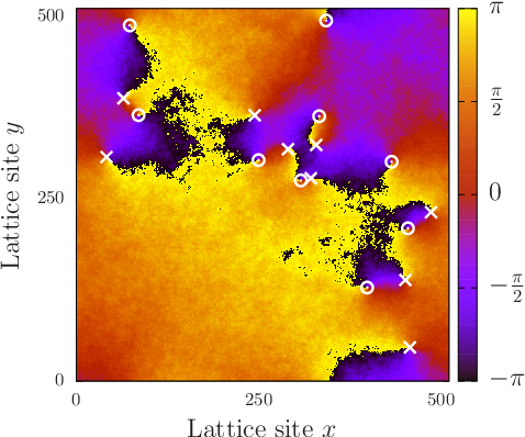
In this article, we present the details of our studies of the relaxation of two and three dimensional dilute Bose gases through stages of superfluid turbulence and the approach of a nonthermal fixed point, by means of simulations in the classical-wave limit of the underlying quantum field theory. In Section II, we summarize the quantum-field theoretical predictions of Refs. [46, 9], in particular for the scaling exponents of the single-particle momentum distribution and compare these with the numerically determined scaling. While we find excellent agreement, our results provide an interpretation of the nonthermal fixed points proposed in Refs. [6, 9] for the case of an ultracold Bose gas: The appearance of nonperturbative infrared scaling reflects the presence of statistically independent vortices, as previously reported in brief in Ref. [16], see also Figs. 3-5. This phenomenon appears to be distinctly different from the weak wave turbulence we observe in the UV part of the spectrum.
In Section III, we describe a model of independent as well as pair-correlated vortical excitations [24] which allows the more refined interpretation of the scaling behavior during the different stages of the evolution presented in Section IV.
We show that the stationary scaling is maintained by the presence of energy (UV) and particle (IR) fluxes, further supporting the analytic theory.
In Section V, we study the power-law distributions of the compressible and incompressible contributions to the flow pattern.
This adds to the clear understanding of the bimodal scaling laws in the overall momentum spectrum.
IR power-law spectra of subdominant compressible excitations suggest the presence of acoustic turbulence [46] on the top of the vorticity-bearing quasicondensate.
In comparison with recent experiments and analytical predictions, the velocity field probability distribution as well as the velocity statistics of individual vortices are studied.
This observable is of great interest, since it has recently been used to experimentally verify a distinction between classical and quantum turbulence [49].
We finally show that the complete decay of the turbulent scaling is anticipated by the appearance of weaker IR power laws reflecting vortex-antivortex pairing correlations.
II Superfluid turbulence as a nonthermal fixed point
We begin with a brief summary of the analytical and numerical results on dynamical fixed points and matter-wave turbulence reported in Refs. [9, 16] before we discuss these results in terms of a statistical model of vortex excitations. Motivated by the original work presented in Ref. [6] nonthermal fixed points of Kadanoff-Baym dynamic equations for time-dependent Green functions were analysed, for the case of an ultracold Bose gas, in Ref. [9]. At these fixed points of the dynamical evolution of the system, the single-particle momentum distribution becomes (quasi-)stationary, . It furthermore exhibits a characteristic universal power-law behavior, i.e., it scales according to
| (1) |
in a certain regime of momenta . Here is some positive, real number and a universal exponent which was determined from the dynamic equations for the field correlation functions. Different exponents resulted in different momentum regimes. Exponents valid in the ultraviolet regime of large were found to correspond to well-known fixed points of weak wave turbulence [46] in the respective systems. In addition to these, new, larger exponents were predicted in the infrared regime of small on the basis of a non-perturbative analysis of the Kadanoff-Baym dynamic equations derived from the two-particle-irreducible (2PI) effective action [6, 7, 8, 9, 10].
Simulations of the classical field equations for a relativistic -symmetric scalar model, for , confirmed the existence of the analytically derived scalings in the infrared regime [6]. As reported in Ref. [16], corresponding simulations were performed for an ultracold, degenerate Bose gas in two and three spatial dimensions which demonstrated that for these systems the infrared scalings predicted in [9] reflect and are caused by the presence of quantized vortical excitations of the superfluid. In this way, the nonthermal fixed points can be related in a clear manner to topological excitations of the interacting coherent matter-wave field which shows that both, weak wave turbulence and macroscopic, topological excitations of the field can be described within a unified field-theoretic approach. Differently expressed, both, weak turbulent flow and non-linear solitary bulk excitations are described in a unified manner as representing a nonthermal critical fixed point of the system. In turn, the approach also implies that superfluid turbulence can be studied in a new way, in the frame of a universal quantum field theoretical approach. We remark that the relation between the new infrared exponents and topological excitations of the background (i.e., condensate) field gains further support by the topological pattern formation described in Ref. [17] for a relativistic -symmetric scalar model, which serves as a particular model for the reheating period after early-universe inflation.
We will discuss in detail vortical excitations in a degenerate Bose gas and their relation to the above nonthermal fixed points. Before this we summarize briefly the relevant results of Refs. [9, 16]. To be specific, throughout this article we consider an ultracold Bose gas of atoms in , space dimensions interacting through -wave collisions which is described by the Hamiltonian
| (2) |
where the time and space dependent fields satisfy Bose commutation relations, and where the coupling in three dimensions is defined in terms of the -wave scattering length . Here and in the following we set , see Appendix B for more details.
II.1 Weak wave turbulence
Suppose the generic case that for sufficiently large momenta occupation numbers are small enough such that for a given coupling the Quantum Boltzmann Equation (QBE)
| (3) | ||||
| (4) |
describes the evolution of under the effects of collisions. In our case, the transition matrix element squared is a numerical constant proportional to and thus independent of momenta. Zeroes of the scattering integral correspond to fixed points of the time evolution within the regime of applicability of the QBE [46]. Most prominent amongst these are the thermal fixed point corresponding to the system in thermal equilibrium and the trivial fixed point where the occupation number is independent of . At both fixed points the scattering integral vanishes and becomes independent of . Note that both, the trivial distribution and the thermal Bose-Einstein distribution in the Rayleigh-Jeans regime, for , show a power-law behavior of the form (1) with and , respectively.
The theory of weak wave turbulence [46] allows to analytically derive further, nonthermal fixed points at which the occupation number obeys a scaling law of the form (1) and, in general, . As in classical turbulence of an incompressible fluid one assumes that universal scaling appears within a certain regime of momenta, the inertial range. According to this picture, outside the scaling regime kinetic energy enters the system from an external source and/or is dissipated into heat, whereas there are no sources and sinks within the inertial interval. Instead, kinetic energy is transported from momentum shell to momentum shell without loss or gain. To a good approximation, this process is described by a continuity equation in momentum space, with a momentum-independent, radially oriented current vector.11 1 Note that justification of this assumption, i.e., locality of the transport, needs to be checked for each particular wave-turbulent solution [46]. A central aspect of weak-wave-turbulence theory is that the QBE can be cast into different such equations [46], for the radial number density and the energy density , ,
| (5) | ||||
| (6) |
Depending on whether the radial particle current or energy current is taken to be independent of , one derives different scaling exponents. The resulting exponents are
| (7) |
These exponents can be obtained by simple power counting: Combining Eqs. (3) and (5) gives the radial relation which implies that stationarity requires to become -independent, i.e. scale like . Counting all powers of in , Eq. (4), in the wave-kinetic regime where the terms of third order in the occupation numbers dominate the scattering integral, this requires . Analogously one infers the exponent from the balance equation (6) for the energy density . Despite this simple procedure, the existence of the respective scaling solutions has to and can be derived rigorously from the QBE by means of Zakharov conformal integral transforms [46]. We note that, similar to classical turbulence, the case is special, where the scaling exponent equals that of a thermal distribution in the Rayleigh-Jeans regime.

II.2 Strong wave turbulence
Given a positive scaling exponent momentum occupation numbers grow large in the IR regime of small . As a consequence, for a given coupling , the QBE fails in this regime, where contributions to the scattering integral which are of higher order than become important.
To find scaling solutions in the IR, an approach beyond kinetic theory is required. This is available through quantum-field dynamic equations derived from the two-particle irreducible (2PI) effective action or -functional [50, 51, 52] beyond the 2-loop order in the expansion of the self-energy. See Ref. [9] for details of the procedure summarized in the following. The 2PI equations include the Dyson equation for the time-ordered Green function (here, we use four-vector notation ), from which a time evolution equation (3) for is derived. As before one considers zeros of the scattering integral which in the dynamic theory reads
| (8) |
Here, , and and are the spectral and statistical components of , respectively, defined in coordinate space by , , . The corresponding contributions to the self energy are defined in terms of through a loop expansion of the 2PI effective action, see Fig. 1. Resumming an infinite set of such loop diagrams contributing to the 2PI effective action [53, 55] leads to a non-perturbative, effectively renormalized coupling in the dynamic equations [6, 9].
To derive the scaling solutions of the dynamic equations for Green functions one assumes separate scaling of its spectral and statistical components according to , , . Here, is the dynamical scaling exponent accounting for a different scaling in as compared to . The scaling exponent is related to by . is derived from the condition that the scattering integral (8) vanishes, making use of Zakharov transformations, while the anomalous scaling exponent remains undetermined by this and, for the first, can be assumed to vanish for the and dimensional cases considered in this paper. The IR scaling exponents for radial quasiparticle flow () and radial energy flow () in dimensions were predicted in Ref. [9] to be
| (9) |
In situations where a quasiparticle picture applies the dynamical exponent corresponds to the homogeneity index of : . In this case the nonperturbatively resummed effective coupling can be related to the diagonal elements of an effective many-body -matrix, in the kinetic Boltzmann formulation. In the scaling regimes this scales as , , where is some constant which fine-tunes the position of the transition from UV to IR scaling: For small and one recovers the UV case discussed in the previous section, i.e., is a constant independent of . For large , the second term in the denominator dominates which, assuming scaling of , implies a power-law behavior and, in turn, the modified scaling (9) of in the infrared regime of small wave numbers as compared to the UV regime discussed before. Physically, the renormalized -matrix implies a reduction of the effective interaction strength in the IR regime of strongly occupied modes [6]. As a consequence, single-particle occupation numbers rise, towards smaller wave numbers, in an even steeper way than in the weak-turbulence regime.


II.3 Wave-turbulent scaling and vortices
in a Bose gas
We now briefly review the relation between wave-turbulent scaling and the appearance of vortical excitations in an ultracold degenerate Bose gas. In [16] the results of semiclassical simulations of the gas dynamics were reported, obtained by solving the classical field equation
| (10) |
in a box with periodic boundary conditions. See Appendix B for details on the simulations and on lattice units. The initial field was prepared by macroscopically populating a few of the lowest momentum modes in the computation such that the resulting condensate density in configuration space varied between zero and some maximum value. Quantum noise is taken into account by adding a small random contribution to each field mode. Vortical excitations were created in large numbers, within shock-waves forming during the non-linear evolution of the coherent matter-wave field. Fig. 3 shows an example of the condensate phase distribution over a numerical lattice in dimensions, with vortices and antivortices indicated by white crosses and circles, respectively. Fig. 5 depicts the location of vortex-ring cores in a -dimensional system. For videos of the evolution see [54]. Both figures show a snapshot of the system at some time after the vortical excitations have formed. At these times, in , part of the vortex-antivortex pairs have re-annihilated with each other already, and in some of the rings have undergone reconnections and also disappeared by shrinking to zero size.
Runs were repeated many times ( times in and times in ) for an ensemble of initial configurations differing by statistical noise. The number of runs was chosen such that the statistical error arising from run-to-run fluctuations was reduced to a value on the order of the size of the symbols used in the figures. In the regime of momenta with large occupation numbers where quantum statistical fluctuations play little role, correlation functions like the spectrum could be computed in a quasi exact way by averaging at a given time over the ensemble. In this way, the flow was analysed in terms of the ensemble- and angle-averaged single-particle spectrum
| (11) |
as a function of radial momentum . Figs. 3 and 5 show this spectrum for and , at the times chosen in Figs. 3 and 5, respectively. Most importantly, these spectra show scaling, Eq. (1), within a range of momenta between about the maximum of the initially occupied momentum modes indicated by the vertical lines and in lattice units. The exponent is in agreement with the field theoretical prediction given in Eq. (7).
It was found that the annihilation processes which eventually destroy the vortical structure while coherence builds up in the system are very slow and thus stabilize the scaling solution over a long time. In particular, only after the last vortex-antivortex pair has annihilated and the last ring shrunk to zero the power law breaks down and a thermal distribution of particles is left over. Characteristic times are for vortex formation, for stabilization of the scaling solution and for the last vortices to annihilate.
III Point- and line-vortex models
As we have seen above, the scaling of the momentum occupation numbers in the IR regime of large wave numbers, predicted within a non-perturbative analysis of strong wave-turbulence, correspond, for - and -dimensional degenerate Bose gases, to the appearance of macroscopic vortical excitations. In the following, we analyse the observed scaling spectra by comparing them to the single-particle momentum distributions for a set of randomly positioned point vortices (vortex lines) in () dimensions. We will show that uncorrelated vortices (vortex lines) are sufficient to yield the infrared scaling with exponent , see Eq. (9). We will also show that beyond this, pair correlations between vortices and antivortices as well as configurations with small rings well separated from each other can give rise to a further scaling exponent deviating from (see Fig. 6).
The point (line) vortex model employed here was introduced by Onsager in 1949 [24]. It describes the complex flow pattern in terms of the statistical mechanics of interacting classical point objects. This model has been constructed as a discrete vorticity approximation of classical fluid turbulence, but it is even more suitable to describe superfluid turbulence consisting of quantized vortices. Further applications include plasma physics or stellar dynamics [56, 57, 58].
In the following, we study the spectrum of a set of vortices, finding different scaling regimes dependent on vortex correlation functions. With this approach, nonthermal fixed points in an ultracold Bose gas can be related to the statistics of vortices. Numerical calculations, sampling field configurations of static randomly positioned vortices, confirm the analytical result. Finally, the velocity probability distribution of a vortex-dominated flow [59, 49] is derived and numerically confirmed.
III.1 Independent vortices in

In two dimensions, an isolated, singly quantized vortex is described by the complex field . As the -dependence of the density only becomes important at small scales on the order of the healing length where our simulations are dominated by thermal excitations, we will omit it in the following and assume to be uniform.
A system of vortices in dimensions can be defined as , where is the single vortex field centered around . We derive the corresponding particle spectrum by considering the hydrodynamic velocity field . Denoting the velocity field of a single vortex as (see Appendix A.1) we can express the mean classical kinetic energy density of the velocity field as
| (12) | |||||
where defines the spatial distribution of vortices with winding number . Here and in the following, denotes an ensemble average over different realizations of the classical field . We derive the low- scaling of from the kinetic-energy spectrum , given by the angle-averaged Fourier transform of , taking into account that at low , the single-particle spectrum is dominated by the superfluid velocity field , i.e.,
| (13) |
One has, from Eq. (12)
| (14) |
with
| (15) |
Below the healing length scale (lattice units), the modulus of the velocity field of a single vortex scales as and is radially symmetric in momentum space. Hence, the angle-averaged single-particle spectrum scales like
| (16) |
Here, denotes the zeroth-order Bessel function and is the distance between vortices and .
III.2 Independent vortex-antivortex pairs
In a two-dimensional superfluid containing vortices and antivortices an effectively attractive force between the two species can lead to pair correlations. We study a signature of this feature in the single-particle momentum spectrum by applying the point vortex model introduced above to the case of vortex-antivortex pairs.
As a first step we calculate the velocity field for a vortex-antivortex pair with the vortex situated at and the antivortex at ,
| (19) |
The squared velocity field far away from the center of the pair can be obtained via a dipole approximation which yields the scaling . Hence, in Fourier space, the pair velocity field scales as for low momenta. In this regime, the vortex-antivortex pair can again be treated as a point-like object with modified velocity scaling. To obtain the infrared scaling of a set of random vortex-antivortex pairs, we define a spatial pair distribution , with denoting the center of the -th vortex-antivortex pair. Then, the analysis performed for random vortices above can be adopted. Therefore, in the case of independently distributed pairs, the approach predicts the infrared scaling of the occupation number to be the same as for a single pair, i.e. .
III.3 Pair correlated vortices in
The considerations from Sect. III.2 are only valid in the far IR (or equivalently for pair size going to zero). In our numerical simulations we found, however, that for large evolution times, a finite minimum distance emerged between vortices and antivortices, and also between vortices with the same circulation, see Sect. V.4. To take into account this observation and to analyse the full spectrum, we go back to writing the distribution as the sum of distributions of vortices and of antivortices. Hence,
| (20) |
with . This allows for a derivation of the kinetic-energy distribution in terms of correlation functions of vortex positions.
We model pairing by the density-density correlation functions
| (21) | |||||
| (22) |
where is the area in which the theta function equals one. The contributions
| (23) |
take into account that, besides the pairing, vortices and antivortices avoid each other in the dilute gas, keeping a minimum distance . This is due to vortex-vortex repulsion and fast vortex-antivortex annihilation on small distances. The functions cancel out in Eq. (20).22 2 If different avoidance scales apply for vortices and antivortices, the terms do not cancel, but the remaining term does not alter the results for pair scaling derived here.
Inserting Eqs. (21), (22) into Eq. (20), evaluating the Fourier transform and angular averaging gives
| (24) |
The expansion of the integral for yields the leading-order result
| (25) |
and, from Eqs. (13) and (14), the same occupation-number scaling as for independent pairs,
| (26) |
At momenta the independent-vortex scaling is restored. We note that the infrared result (26) can also be achieved by choosing more general pair correlations of the form , with and , which is closer to our numerical observations and includes the case of a fixed “binding length” . As before, pair scaling is found for , critical scaling for , irrespective of .

We supplement our discussion of scaling in the point vortex model with numerical data obtained by averaging over an ensemble of field configurations in dimensions. These configurations were constructed by multiplying uncorrelated single-vortex fields centered at positions according to the probability distribution
| (27) |
with , where we neglect that unpaired vortices avoid each other, i.e., choose . They do not represent stable solutions of the classical field equation nor do they contain sound-wave and related excitations yet which would build up through the interactions of the field and the vortices.
The resulting momentum spectrum is presented in Fig. 7. Three scaling regimes can be observed. At low momenta the power law is consistent with the existence of random vortex pairs . Above , choosing (lattice units), the distribution exhibits the scaling of an ensemble of independent vortices, , while at momenta larger than the healing-length scale one observes the vortex-core scaling . The above results reflect that in a vortex dominated flow, particles with low momenta are found far away from vortex cores. In the case of pairing, the flow field far away from the cores is given by the field of a vortex pair, and the low-momentum scaling follows the pair-field scaling. Particles closer to the vortex cores pick up a higher momentum. Above the field will be dominated by the field of a single vortex. Note that Fig. 7 shows the result of a numerical calculation in which we have sampled field configurations of random static vortices. Dynamical simulations of the classical field equation Eq. (10) will be shown in Sect. IV.
We close with recalling the picture Onsager developed in Ref. [24] of thermodynamic equilibrium states of a fixed number of vortices and antivortices in two dimensions. He used the Hamiltonian of vortical flow in two dimensions [61],
| (28) |
to describe the dynamics of a system of vortices in a superfluid which hence behave like a Coulomb gas. Here, the position of the -th vortex is denoted as . Due to the fact that the and coordinates of each vortex are canonical conjugates, phase space is identical with configuration space of the vortex positions. Hence, for vortices moving in a volume the total phase space is given by . The Hamiltonian (28) implies that low-energy configurations feature vortices of opposite sign close to each other, whereas high-energy configurations require vortices of equal sign to group. Due to these constraints, the number of configurations available for the system at a given energy decreases towards high and low energies, with a maximum at some intermediate . According to Boltzmann, the entropy is and the inverse temperature is positive for and negative for . It follows that positive-temperature states are characterized by vortex-antivortex pairing, while negative-temperature states feature vortices of the same circulation to cluster. At the point of maximum entropy and infinite temperature, Onsager expected a state of uncorrelated vortices and antivortices. This understanding of the nonthermal fixed point as a quasi-equilibrium state of vortices corroborates our result that the IR scaling behavior at the fixed point corresponds to the appearance of topological excitations.
III.4 Vortex loops in

We now consider the three-dimensional case of vortex lines and loops. A formulation similar to the Onsager point vortex model in Sect. III.1 is possible [62, 63, 34]. See also Refs. [64, 65, 66, 67] for an extension including the dynamics of tangles of vortex lines.
We write the classical kinetic energy spectrum of the velocity field in terms of the vorticity density
| (29) |
as
| (30) |
The vorticity is vanishing everywhere but on the vortex lines, i.e., assuming individual vortex loops,
| (31) |
In this expression, the vortex filaments are represented by the connected curves , parametrized by the one-dimensional coordinate , being the arc length of filament . The loops are closed, , possibly also accross the walls of the 3-dimensional volume in accordance with periodic boundary conditions. is the tangent vector along the filament at , of unit length . We parametrize the -th vortex loop in terms of a single center coordinate and a relative curve, and write the vorticity as
| (32) |
Hence, in Fourier space,
| (33) |
where is the Fourier transform of the vorticity of the -th vortex loop, given by
| (34) |
The ensemble-averaged vorticity becomes
| (35) |
Assuming that the shapes of the individual vortex loops are statistically independent of their position, it follows that . If the loops are also uncorrelated among themselves, then . Hence, for statistically identical loops,
| (36) |
which means that the vorticity spectrum scales in the same way as the average vorticity of a vortex loop centered at the origin. Finally, the scaling of the momentum spectrum follows from that of the angle-averaged vorticity,
| (37) |
For the case of two straight parallel vortex lines of opposite circulation Eq. (36) is evaluated in Appendix A.2, for an ensemble of such paired lines in Appendix A.3. Making use of the procedure developed there, the case of circular vortex rings of radius is discussed in Appendix A.4. For the latter, the resulting angle-averaged momentum spectrum scales like for momenta and for momenta . To include effects from squeezed vortex loops, we consider elliptical filaments. The ellipse is defined by a major radius and minor radius . In Fig. 8, the angle-averaged momentum spectrum of an elliptical vortex loop is shown. Three scaling regimes can be distinguished. For the lowest momenta, one has , which equals the infrared scaling for a vortex ring. For momenta , one finds , which coincides with the infrared scaling of two anti-circulating vortex lines (see App. A.2). For the ellipse, above , the momentum distribution scales like , which is the same as the high-momentum scaling of a vortex ring (see App. A.4) or of a pair of straight vortex lines (App. A.3).
III.5 Velocity distribution

The vortex model can provide insight into another observable accessible in our numerical simulations, the velocity distribution. See Refs. [59, 68, 69, 70] for discussions of the velocity distribution and Ref. [49] for recent experimental results. As discussed above, the velocity field scales, far away from any core, as , with for a single vortex and for a vortex-antivortex pair in two dimensions. The velocity probability distribution is calculated as , with spatial vortex distribution function . For a uniform distribution , it follows after angular averaging that
| (38) |
It is numerically convenient to calculate the probability density of a single component of the field, e.g.
| (39) |
In Fig. 9, the corresponding velocity distribution is shown. In accordance with the analytical predictions two scaling regimes are observed. At low momenta the velocity field follows the scaling of vortex-antivortex pairs, whereas at higher momenta the distribution reflects a random distribution of vortices.
IV Bose gas approaching the nonthermal fixed point
In this section we return to the process of the formation of vortical excitations and of the Bose gas approaching the nonthermal fixed point characterized by the wave-turbulent scaling solutions discussed in Sect. II and Refs. [9, 16]. Thereby we first focus on the evolution of the single-particle momentum distributions and the emergence of nonthermal power laws. We relate these to structure formation in the form of vortical excitations. In order to identify in a clearer way the relevant processes in approaching the fixed point we compute the fluxes in momentum space. Remarkably, we find that the appearance of the particle scaling exponent in the IR and of the energy exponent in the UV are compatible with predictions based on general arguments of irreversibility as well as energy and number conservation in a collision process [46].
IV.1 Time evolution of the single-particle spectrum


As discussed in Sect. II.3, vortical excitations can be created in large numbers, within shock waves forming during the non-linear evolution of the coherent matter-wave field. Figs. 10 and 11 show the angle- and ensemble-averaged radial momentum spectra, Eq. (11), for a Bose gas in a box with periodic boundary conditions, in and dimensions, respectively. Four snapshots are shown, taken at the dimensionless times as indicated in each panel. See Appendix B for details on the simulations and on lattice units. The initial field configurations were prepared by macroscopically populating a few of the lowest momentum modes in the computation such that the resulting condensate density in configuration space varied between zero and some maximum value. In Figs. 10 and 11, the panels representing the earliest times show the system after a brief initial evolution during which momentum is rapidly transported from the few initially occupied modes near zero over a comparatively large range of wave numbers.
Shortly after this, vortical excitations are created which immediately causes the spectrum in dimensions to exhibit a power-law behavior within a range of momenta , see the upper right panel of Figs. 10. Subsequently, the evolution slows down and a quasi-stationary period is entered. During an intermediate stage (bottom left panel of Fig. 10 and upper right panel of Fig. 11) of the vortex-bearing phase two distinct power laws develop which are in excellent agreement with the analytical prediction in Eqs. (7) and (9). While in the ultraviolet the exponent exhibits weak wave turbulence, Eq. (7), in the infrared, the exponent confirms the field theory prediction , cf. Eq. (9). More specifically, in two dimensions, at , one observes scaling exponents within a range of momenta and within a range of momenta , see the lower left panel of Figs. 10. At , within a range of momenta , see the lower right panel of Figs. 10. In dimensions, at , one observes within a range of momenta and within a range of momenta , see the upper right panel of Figs. 11. At , within a range of momenta , see the lower left panel of Figs. 11. The appearance of the bimodal power laws corroborates results for a relativistic model reported in Refs. [6, 10].
During the ensuing evolution, the weak-wave-turbulence scaling decays towards , reflecting a thermal UV tail. Note that in , the weak-turbulence exponent is identical to that in thermal equilibrium in the Rayleigh-Jeans regime, [46]. In we observe, at late times, a change of the infrared scaling behavior from to , pointing to the development of pairing correlations, cf. Sects. III.3, III.4, and Sect. V.4 below. More specifically, at , one observes a scaling exponent within a range of momenta , see the lower right panel of Figs. 11.
At late times, after the last vortical excitations have disappeared, we observe the entire spectrum to become thermal, i.e., exhibit Rayleigh-Jeans scaling with (not shown). We emphasize that thermal scaling of the single-particle occupation number with applies despite the fact that quasiparticles with a linear dispersion are expected to thermalize in the regime of wave numbers smaller than the inverse healing length () and (). In the Bogoliubov approximation this is seen by taking into account the power-law dependence of the coefficients which contribute to [9].
We are going to study more details of the time evolution of the system in a forthcoming publication and focus in the remainder of this paper on properties of the stationary scaling distributions. An important question in this context is, why the system selects the particular exponents and from the set of four possible exponents given in Eqs. (7) and (9). For this, the fluxes underlying the stationary but non-equilibrium distributions are relevant.
IV.2 Fluxes


The timeline of distributions shown in Figs. 10 and 11 suggests that the evolution of the gas involves a transport process from intermediate momenta around both towards lower and higher wave numbers, building up a bimodal power-law distribution. To describe the character of these transport processes we plot, in Fig. 12 for (upper set of four panels) and (lower set), the radial particle and kinetic-energy flux distributions and , respectively. Note that the radial particle flux density is multiplied by to have the same units as the energy flux density . These flux densities are defined through the balance equations (5) and (6), respectively, with kinetic energy density . The initial stage is governed by an infrared particle transport towards larger , also causing a flux of interaction energy. At intermediate times, changes sign. This is accompanied by a positive kinetic energy transport in the UV, as observed in two-dimensional simulations in Ref. [71].
We emphasize that the negative particle flux in the IR and the positive kinetic-energy flux in the UV coincide with the appearance of the bimodal momentum distributions in Figs. 10 and 11 (bottom left panels). Although the derivation of the IR exponents requires the full dynamical theory with non-perturbatively resummed self-energies, the signs of the fluxes correspond to the respective scaling exponents, i.e., in the IR, and in the UV, cf. Sect. II.1. Moreover, at late times, the kinetic-energy flux vanishes due to a thermalized UV momentum distribution, but still reshuffles particles and therefore interaction energy, keeping the system out of equilibrium close to the nonthermal fixed point.
We finally remark that, as discussed in detail in Ref. [46], one can show on the general grounds of the Boltzmann -theorem that a necessary condition for a non-equilibrium stationary distribution in our systems is energy damping in the region of large . Moreover, energy and particle number conservation in the interaction of different momentum modes can be shown to imply the existence of at least one more sink, i.e., a region where the right-hand sides of Eq. (5) effectively has an additional damping term , with negative . In between these sinks, a source region supplies the input to the bidirectional flux pattern towards the UV and IR. It was shown, moreover, in Ref. [46], within wave-kinetic theory, that generally, a positive, -independent flux transports energy, while a negative flux transfers particles, . The only exception is the case of where the thermal and the weak-wave-turbulence exponent can not be distinguished. Remarkably, this pattern remains valid in our case, beyond the UV weak-wave-turbulence regime, in the IR region where the exponent emerges from a fixed point of the full dynamic equations. As already pointed out in Ref. [9], however, the derivation of the IR exponent requires the existence of a sufficiently well defined quasi-particle dispersion relation, suggesting a treatment in terms of the Quantum Boltzmann equation with a momentum dependent scattering matrix element to be applicable.
From this point of view, the negative flux and scaling in the IR and the positive flux and weak wave turbulence in the UV, as observed in the numerics, emerge as a necessary consequence of conservation laws and transport processes described by wave-kinetic transport equations.
V Vortices, acoustic turbulence and the departure from the fixed point
In this last section we analyse the single-particle momentum spectra obtained in our numerical simulations in view of their interpretation in terms of vortical excitations and wave-turbulence as implied by the point- and line-vortex models introduced in Sect. III. For this we first decompose the flow pattern of the system which has closely approached the nonthermal fixed point, into transverse (incompressible) and longitudinal (compressible) contributions. In this way we can show that the IR scaling is dominated by the incompressible part while in the UV the particles mainly belong to the compressible as well as a quantum pressure components. We find a further scaling exponent for the subdominant compressible component in the IR which is interpreted as a signature of acoustic turbulence.
Moreover, going beyond the results presented in [16] we identify signs of pair formation in the final stage. The scaling caused by this goes beyond the predictions from dynamical quantum field theory summarized in Section II, and we interpret it as a signature for the system leaving the fixed point again for final thermalization.
V.1 Superfluid turbulence and statistics of vortices


To exhibit vortical flow and define the decomposition we use the polar representation of the field in terms of the density and a phase angle . This allows to express the particle current in terms of the velocity field .
With this, we decompose the kinetic-energy spectrum following Ref. [29, 30], splitting the total kinetic energy as into a ‘classical’ part
| (40) |
and a ‘quantum-pressure’ component
| (41) |
The radial energy spectra for these fractions involve the Fourier transform of the generalised velocities and ,
| (42) |
Following Ref. [29, 30], the velocity , which due to the multiplication of with the density becomes regularized and can be Fourier transformed, is furthermore decomposed into ‘incompressible’ (divergence free) and ‘compressible’ (solenoidal) parts, , with , , to distinguish vortical superfluid and rotationless motion of the fluid. For comparison of the kinetic-energy spectrum with the single-particle spectra , we determine occupation numbers corresponding to the different energy fractions as
| (43) |
The resulting spectra , , and add up to , which agrees with the single-particle spectrum up to small corrections, see Appendix C.
In Figs. 13 and 14, we depict the momentum distributions of the occupation numbers , , and , together with the previously shown total single-particle spectrum , each at a late time when the system is close to the fixed point, i.e., shows the predicted scaling both in the IR and the UV. Red circles denote , filled blue squares , and open grey squares . Qualitatively, the results are similar for and .
In the range of large wavenumbers, the spectrum is dominated by the compressible and quantum-pressure components. The scaling of these excitations exhibits the weak-wave-turbulence exponent . For smaller wave numbers the scaling changes to . The decomposition into the various components now shows that this switching to a different scaling in the IR is clearly due to the take-over of a different character of the excitations with a modified flow pattern accounted for by the incompressible (solenoidal) component of . The fact that in this regime contributions from vortical flow dominate is in accordance with our interpretation of the strong IR scaling by a model of an ensemble of vortical excitations. As we have discussed in the previous section the analytically predicted infrared power laws are consistent with a finite density of independent vortices and antivortices () or vortex lines ().
Moreover, we find that the compressible component in the IR represents the second strongest contribution to the flow and develops a nonthermal scaling as . We will discuss this result in more detail in Sect. V.2 below.
For momenta larger than about for and for the compressible and quantum-pressure components dominate the momentum distributions. In the regime of intermediate momenta, above the scale with the mean inter-vortex spacing, where the incompressible flow and the rest are of roughly equal strength one finds a scaling of approximately , corresponding to for both the two- and the three-dimensional case. Scaling with this exponent, which is the same as in classical Kolmogorov turbulence in an incompressible fluid, has been found in simulations of superfluid turbulence in before [29, 30, 31, 32, 33, 20, 21, 34, 72]. In some of these cases, turbulent flow appeared in the time evolution of a system starting from a Taylor-Green configuration of vortex line tangles. We emphasize that our configuration after the creation of vortical excitations resembles more a state of the kind usually termed chaotic turbulence. It is unclear whether chaotic turbulence can be related to classical Kolmogorov turbulence as this does not bear near-classical bundles of equal-orientation vortex lines. Nonetheless we observe such scaling in the range of intermediate momenta where the interplay between the incompressible and compressible components is most pronounced.
V.2 Acoustic turbulence


The IR scaling of the compressible component (blue filled squares) in Figs. 13, 14, and also Fig. 18 below suggests an interpretation in terms of acoustic turbulence [46, 37, 38, 42] and corroborates the numerical findings reported in Ref. [73]. The scaling is persistent until late times, see, e.g., Fig. 18, but decays after the vortices have disappeared. To check that the nonthermal scaling of the incompressible component is not an artefact of the decomposition of the vortical flow into compressible and incompressible parts, we show the momentum spectrum for an average over selected runs in , see Fig. 15 (lower panel), where the snapshot is taken shortly after the last vortex ring has disappeared. One can observe that acoustic turbulence can survive for a limited period, , beyond the time when vortical excitations are negligible. In the case of , the effect is weaker but still present, see Fig. 15 (upper panel), where we show the averaged spectrum shortly after the last vortex-antivortex annihilation. Our interpretation of this finding is that acoustic turbulence coexists with the dominant vortical flow. It is driven by vortex motion and especially vortex annihilation processes, which are known to produce compressible excitations. In , signatures of acoustic turbulence are less pronounced, which we attribute to reduced vortex dynamics or, equivalently, weaker driving of compressible excitations.
V.3 Vortex velocities


We furthermore investigated the velocity-field probability distribution in the turbulent regime to compare our data with the expectations summarized in Sect. III.5. In dimensions, see Fig. 16, the results corroborate theoretical and experimental results reported in Refs. [59, 49, 74, 75]. The low-momentum distribution is characterized by Gaussian statistics, whereas the UV regime clearly shows scaling predicted by the model of randomly distributed, uncorrelated vortex lines, see Eq. (39). Note that even at late times, when vortex rings shrink in size, no signs of vortex pairing, , can be seen in the velocity distribution. This is due to dominating Gaussian fluctuations in the low momentum region. In dimensions, see Fig. 17, we compare the velocity-field distribution with the velocity distribution of the positions of the individual vortices. Similar to the three-dimensional case the IR part of the velocity-field distribution is characterized by Gaussian statistics, whereas the UV regime shows single-vortex scaling [59]. The vortex velocity distribution is obtained from the statistical analysis of a vortex-tracking algorithm which is designed to detect regions of low density accompanied by a winding number equal to one. The method is analogous to the experimental set-up of Ref. [49], where particles are trapped inside vortex cores to study vortex velocities in . In agreement with the experiment, Fig. 17 shows that Gaussian random motion is suppressed for vortices, but scaling clearly persists. In this way, quantum turbulence can be distinguished from classical turbulence, where a continuous distribution of vorticity favors a Gaussian velocity distribution.
V.4 Pairing and departure from the fixed point


In Fig. 18 we show the decomposition of the single-particle spectrum into the previously defined incompressible, compressible, and quantum-pressure components, see Eq. (43), for the 3-dimensional system at , as in the lower right panel of Fig. 11. At this time, only a small density of vortex rings has survived, which decays under the influence of the noise field, cf. also Refs. [76, 77]. During the period when only a few small vortex rings remain one can observe a decrease of the infrared scaling exponents of the occupation number and its incompressible part to the value . Since vortical excitations are still dominating the spectrum, we can interpret this observation in terms of the statistical point vortex model introduced in Sect. III, as vortex-antivortex pair correlations, see Sect. III.4. This is consistent with the snapshots of individual runs showing small vortex ellipses (see inset of Fig. 18). The scaling transition can be identified with the scale , with estimated minor radius .
Fig. 19 shows the average occupation number spectrum at in dimensions, as in the lower right panel of Fig. 10. In the average over all generated runs pairing effects can hardly be observed. However, for selected runs with small maximum pair correlation length , as introduced in Sect. III.3, the pair scaling appears. We find that in the selected runs ( of total number of runs), at the chosen point of time one or at most a few vortex-antivortex pairs with pairing length smaller than the distance between pairs are present. This constitutes the final period of the evolution, shortly before the last pair has disappeared through mutual annihilation and the system fully thermalizes. The generic configuration in dimensions during the preceding time interval of critical slowing down close to the nonthermal fixed point is characterized by randomly positioned vortices and antivortices, with pairing correlations nevertheless present. Pairing is seen in the density-density correlation function between vortices and antivortices shown in Fig. 20, from which we read off a largest scale , cf. Sect. III.3. This implies pair scaling below , not visible in the few (black) full circles in Fig. 19.

We observe that, in , scattering between the vortices of equal and opposite circulation can lead to the increase of the pairing length between correlated vortices and antivortices. This is in contrast to the situation for where the scattering between vortex rings rarely leads to an increase in the size of the rings. It is energetically advantageous for the rings to shrink in size, and thus, at a particular late time of the evolution the presence of separated small rings is generic and ”pairing” is seen in the spectrum.
In summary, our analysis gives a picture of the necessary conditions and the character of the nonthermal fixed point. It also shows that pairing effects are a first signature for the system leaving this fixed point again for the final move to thermal equilibrium.
VI Summary
We have studied in detail superfluid turbulence in two- and three-dimensional dilute Bose gases by means of simulations in the classical-wave limit of the underlying quantum field theory. A focus is set on the identification and characterization of stationary scaling solutions, in particular for single-particle momentum distributions. Characteristic exponents of corroborate the analytical predictions made in Ref. [9]. Our findings suggest that local field expectation values and short- to intermediate-range coherence, including topological excitations, are at the basis of the infrared power laws predicted within a full nonperturbative dynamical field theory [6, 7, 8, 9, 10, 17] employing two-particle-irreducible effective action techniques.
We have shown that the stationary scaling is maintained by the presence of particle (IR) and energy (UV) fluxes, originating at intermediate scales and directed towards the low- and high-frequency limits, respectively. The respective fluxes were found to be consistent with the particular scaling exponents of the momentum distribution in the respective regimes. Our main result is the identification of the nonthermal fixed-point with the appearance of topological excitations in the system. We could successfully employ statistical models of point vortices in two dimensions and vortex rings in three dimensions to interpret the IR scaling exponent of the spectra. Moreover, we observed in our simulations, during the final thermalization stage, decay of the turbulence scaling into a scaling derived from the assumption of vortex-antivortex pairing. To characterize further the bimodal power spectra developed close to the nonthermal fixed point we have analysed the decomposition of the overall flow pattern into compressible and incompressible components. We found that the IR power spectra of underlying compressible excitations suggest an understanding in terms of acoustic turbulence on top of the vorticity-bearing quasicondensate. Finally, to compare with the results of recent experiments and analytical predictions, the velocity-field probability distribution as well as the velocity statistics of individual vortices has been studied. This observable is of great interest, as it can be used to experimentally distinguish between classical and quantum turbulence.
The connection of QT phenomena with ab-initio dynamical field theoretic methods points a way to unified analytical studies of turbulence. Moreover, it provides hints of how the proposed nonthermal fixed points in relativistic systems [6, 7, 8, 10, 14] are realized in nature. A manifestation of the approach of a nonthermal fixed-point in terms of quasi-solitary pattern formation and charge separation in a relativistic scalar model has recently been reported in Ref. [17].
Experimental studies of universal phenomena in nonequilibrium dynamics of ultracold atoms have great potential since universal effects do not depend significantly on initial conditions and details of the system. Following this idea, our numerical protocol was chosen such that an experimental verification of our findings is within reach of present-day cold-atom experiments. The study of turbulence in ultracold gases may have great impact on many other fields of physics. Prominent examples are strongly correlated nuclear matter produced in heavy-ion collisions and early-universe cosmology.
Acknowledgements.
T. G. and D. S. thank J. Berges and C. Scheppach for collaboration on related work. The authors thank J. Berges, N. Berloff, E. Bodenschatz, M. J. Davis, G. Falkovich, S.-C. Gou, H. Horner, R. Kerr, G. Krstulovic, M. K. Oberthaler, J. M. Pawlowski, B. Shivamoggi, B. Svistunov, and M. Tsubota for useful discussions. They acknowledge support by the Deutsche Forschungsgemeinschaft (GA 677/7,8), by the University of Heidelberg (FRONTIER, Excellence Initiative, Center for Quantum Dynamics), by the Helmholtz Association (HA216/EMMI), and by the University of Leipzig (Grawp-Cluster). The authors furthermore thank KITP, Santa Barbara, for its hospitality. This research was supported in part by the National Science Foundation under Grant No. PHY05-51164.Appendix A Vortical excitations in a superfluid
A.1 Single vortex in dimensions
A singly quantized vortex with circulation in two dimensions is described, in polar coordinates, by the solution of the Gross-Pitaevskii equation (10), where is real and approaches the square root of the bulk density for large distances from the vortex core where . A vortex is a stationary solution of Eq. (10), evolving as with . The velocity field of the vortex is
| (44) |
The Fourier transform of this field can be conveniently evaluated by the help of the first-order Bessel function, , as
| (45) |
A.2 Straight vortex line in
Based on Eq. (31), we calculate the vorticity of two straight vortex lines in three dimensions, with circulation , , placed at positions and in the - plane and relate it to the momentum spectrum, see Eq. (37). The lines are parametrized by
| (46) |
with . In Fourier space, the vorticity density, defined in Eq. (29), reads
| (47) |
The vorticity spectrum follows from Eq. (31),
| (48) |
Hence, for co-rotating vortex lines ()
| (49) |
while for counter-rotating vortex lines () one obtains
| (50) |
In order to be able to take the angle average over we regularize the delta distribution, giving it a finite width . The angle average of Eq. (49) then reads
| (51) | |||||
where is the length of the system in -direction and . One obtains the scaling behaviour
| (52) |
which is the scaling of a single line. With Eq. (37), we conclude . Following the same reasoning, the angle average of Eq. (50) is given as
| (53) |
For
| (54) |
which gives . For
| (55) |
which gives . These scalings are confirmed in Fig. 21.


A.3 Ensembles of parallel vortex lines in
In Sects. III.2 and III.3, we have discussed the scaling of the momentum distribution for ensembles of independent and pair correlated vortices in two dimensions, respectively. In this appendix we generalize the scaling derived above for straight vortex lines to the case of many such lines in . We derive an expression for the momentum spectrum of a system of straight vortex lines oriented along the direction. The average vorticity squared is given by Eq. (35) where are vectors in the two-dimensional - plane pointing to the -th vortex line with circulation . The vorticity of the single line is
| (56) | |||||
Hence, Eq. (35) has the same form as Eq. (15) for ,
| (57) |
up to a term, which arises from the infinite extent of the vortex lines in -direction. As in App. A.2, we regularize the delta distributions, and averaging (57) over solid angles yields
| (58) |
which is analogous to Eq. (16) in two dimensions. As the position of the -th vortex line is determined by , statistical averaging of (58) can be done in the same way as in .
A.4 Vortex ring in
A vortex ring with radius lying in the - plane can be parametrized as
| (59) |
with . In Fourier space, similar steps as above lead to the angle-averaged vorticity density
| (60) |
Evaluating the integral numerically shows that the vorticity scales like for and for , corresponding to and . This is shown in Fig. 22. Both scalings are also found in the momentum spectrum of a vortex ellipse, discussed in Sect. III.4.
Appendix B Semiclassical field simulations
In this paper, a dilute superfluid gas of Bosons of mass is considered, with contact interactions quantified by a coupling constant . Its dynamics is described, in the classical wave limit, by the Gross-Pitaevskii equation (GPE) (10). We use units where . We consider the gas to be contained in a box of size , , with periodic boundary conditions. In , the coupling constant is related to the -wave scattering length by . In , one has where is the chemical potential and is a scattering length in two dimensions which, for a gas of hard-spheres of radius is given by , with the Euler-Mascheroni constant [78, 79, 80]. For a two-dimensional gas created by trapping a three-dimensional one tightly in one dimension, with harmonic-oscillator length , the effective 2D scattering length is given by , where [81]. Diluteness implies that , the interparticle spacing being determined by the mean density .
The initial values for the real and imaginary parts of the field are randomly chosen from a Gaussian distribution with width , centered around , where is the occupation number at time and is a random phase angle. Correlation functions including are obtained by averaging over many trajectories. To induce transport from small to large wave numbers, only a few modes near are chosen to be macroscopically occupied at the initial time, . Such an initial state can be prepared, e.g., by Bragg scattering of photons from a Bose-Einstein condensate.
Our numerical simulations are performed on space-time lattices with side lengths , with lattice spacing and in total gridpoints. We use periodic boundary conditions and for and for . Eq. (10) is written in terms of the dimensionless variables , and . All quantities in the figures are either dimensionless or shown in lattice units, with the length unit given by . The dimensionless lattice momenta are .
In order to relate our simulations to a typical situation in experiment, we give parameters for Rb-87. We estimate the total energy of the gas in equilibrium to be given by the interaction energy which, by equipartition is related to the temperature, . At the transition to degeneracy the thermal de Broglie wave length is of the order of the interparticle spacing and hence . Inserting this into the expression for the interaction energy allows to express the lattice spacing in terms of the density and the scattering length as
| (61) |
Inserting parameters for a typical Rb-87 experiment in , viz., nm, kg, m-3 we obtain m. Hence, time scale as s. Our lattice time typically runs until , which therefore represents a realistic observation timescale in experiments. Typical parameter choices in our simulations are , , for and , , for .
Appendix C Decomposition of

In Sect. V.1, we have defined occupation numbers corresponding to the incompressible, compressible and quantum pressure components of the kinetic energy. Numerically, the resulting spectra , , and add up to which is equal to the full single-particle spectrum up to small corrections. In particular, the scaling behavior emerges as the same for both, and . To make this more explicit, we calculate in terms of generalized velocities v,q,
| (62) |
denotes the real part and the Fourier transform. The middle term vanishes since the expectation value is purely imaginary due to isotropy. It follows that
| (63) |
Since phase and phase velocity are expected not to be correlated, the main contribution to the 4-point correlation functions is assumed to arise from terms of the form , v,q. In the superfluid regime, the phase of the field is a slowly varying function in position space. Therefore, -terms are strongly peaked at zero momentum, effectively acting as regularized delta functions under the convolution. Hence,
| (64) |
This approximative identity is supported by Fig. 23.
References
- [1] U. Frisch, Turbulence: The Legacy of A. N. Kolmogorov (Cambridge University Press, Cambridge, UK, 1995).
- [2] L. F. Richardson, Proc. Roy. Soc. Lond. A 97, 354 (1920).
- [3] A. N. Kolmogorov, Dokl. Akad. Nauk. USSR 30, 299 (1941)[Sov. Phys. Dokl. 10, 734 (1968)]; reprinted in Proc. Roy. Soc. Lond. A, 434, 9 (1991).
- [4] A. M. Obukhov, Izv. Akad. Nauk S.S.S.R., Ser. Geogr. Geofiz. 5, 453 (1941).
- [5] R. Micha and I. I. Tkachev, Phys. Rev. Lett. 90, 121301 (2003).
- [6] J. Berges, A. Rothkopf, and J. Schmidt, Phys. Rev. Lett. 101, 041603 (2008).
- [7] J. Berges and G. Hoffmeister, Nucl. Phys. B813, 383 (2009).
- [8] J. Berges, S. Scheffler, and D. Sexty, Phys. Lett. B681, 362 (2009).
- [9] C. Scheppach, J. Berges, and T. Gasenzer, Phys. Rev. A 81, 033611 (2010).
- [10] J. Berges and D. Sexty, Phys. Rev. D 83, 085004 (2011).
- [11] P. B. Arnold and G. D. Moore, Phys. Rev. D 73, 025006 (2006a).
- [12] P. B. Arnold and G. D. Moore, Phys. Rev. D 73, 025013 (2006b).
- [13] A. H. Mueller, A. I. Shoshi, and S. M. H. Wong, Nucl. Phys. B760, 145 (2007);
- [14] M. Carrington and A. Rebhan, Eur. Phys. J. C71, 1787 (2011).
- [15] K. Fukushima and F. Gelis, Nucl. Phys. A 874, 108 (2012).
- [16] B. Nowak, D. Sexty, and T. Gasenzer, Phys. Rev. B 84, 020506(R) (2011).
- [17] T. Gasenzer, B. Nowak, and D. Sexty, Phys. Lett. B 710, 500 (2012).
- [18] W. P. Halperin and M. Tsubota, eds., Progress in Low Temperature Physics Vol. 16: Quantum Turbulence (Elsevier, Amsterdam, 2008).
- [19] R. J. Donnelly, Quantized Vortices in Liquid He II (CUP, Cambridge, 1991).
- [20] T.-L. Horng, C.-H. Hsueh, and S.-C. Gou, Phys. Rev. A 77, 063625 (2008).
- [21] T.-L. Horng, C.-H. Hsueh, S.-W. Su, Y.-M. Kao, and S.-C. Gou, Phys. Rev. A 80, 023618 (2009).
- [22] V. Yukalov, Las. Phys. Lett. 7, 467 (2010).
- [23] C. J. Foster, P. B. Blakie, and M. J. Davis, Phys. Rev. A 81, 023623 (2010).
- [24] L. Onsager, Nuovo Cim. Suppl. 6, 279 (1949).
- [25] R. P. Feynman, in Progress in Low Temperature Physics Vol 1., edited by C. J. Gorter (North Holland, Amsterdam, 1955), p. 17.
- [26] J. Maurer, and P. Tabeling, Europhys. Lett. 43, 29 (1998).
- [27] S. R. Stalp, L. Skrbek, and R. J. Donnelly, Phys. Rev. Lett. 82, 4831 (1999).
- [28] W. F. Vinen and J. J. Niemela, J. Low Temp. Phys. 128, 167 (2002).
- [29] C. Nore, M. Abid, and M. E. Brachet, Phys. Rev. Lett. 78, 3896 (1997a).
- [30] C. Nore, M. Abid, and M. E. Brachet, Phys. Fluids 9, 2644 (1997b).
- [31] T. Araki, M. Tsubota, and S. K. Nemirovskii, Phys. Rev. Lett. 89, 145301 (2002).
- [32] M. Kobayashi and M. Tsubota, Phys. Rev. Lett. 94, 065302 (2005a).
- [33] M. Kobayashi and M. Tsubota, J. Phys. Soc. Jpn. 74, 3248 (2005b).
- [34] M. Tsubota, J. Phys. Soc. Jpn. 77, 111006 (2008).
- [35] G. Krstulovic and M. Brachet, Phys. Rev. E 83, 066311 (2011).
- [36] E. Levich and V. Yakhot, J. Phys. A: Math. Gen. 11, 2237 (1978).
- [37] Y. Kagan, B. V. Svistunov, and G. V. Shlyapnikov, Zh. Eksp. Teor. Fiz. 101, 528 (1992) [Sov. Phys. JETP 74, 279 (1992)].
- [38] Y. Kagan and B. V. Svistunov, Zh. Eksp. Teor. Fiz. 105, 353 (1994) [Sov. Phys. JETP 78, 187 (1994)].
- [39] Y. Kagan and B. V. Svistunov, Phys. Rev. Lett. 79, 3331 (1997).
- [40] N. G. Berloff and B. V. Svistunov, Phys. Rev. A 66, 013603 (2002).
- [41] B. Svistunov, in Quantized Vortex Dynamics and Superfluid Turbulence, edited by C. Barenghi, R. Donnelly, and W. Vinen (Springer, Berlin, 2001).
- [42] E. V. Kozik and B. V. Svistunov, J. Low Temp. Phys. 156, 215 (2009).
- [43] C. N. Weiler, T. W. Neely, D. R. Scherer, A. S. Bradley, M. J. Davis, and B. P. Anderson, Nature 455, 948 (2008).
- [44] E. A. L. Henn, J. A. Seman, G. Roati, K. M. F. Magalhães, and V. S. Bagnato, Phys. Rev. Lett. 103, 045301 (2009).
- [45] J. A. Seman, E. A. L. Henn, R. F. Shiozaki, G. Roati, F. J. Poveda-Cuevas, K. M. F. Magalhães, V. I. Yukalov, M. Tsubota, M. Kobayashi, K. Kasamatsu, and V. S. Bagnato, Laser Physics Letters 8, 691 (2011).
- [46] V. E. Zakharov, V. S. L’vov, and G. Falkovich, Kolmogorov Spectra of Turbulence I: Wave Turbulence (Springer-Verlag, Berlin, 1992).
- [47] S. Nazarenko, Wave turbulence, no. 825 in Lecture Notes in Physics (Springer, Heidelberg, 2011).
- [48] A. Newell, Ann. Rev. Fluid Mech. 43 (2011).
- [49] M. S. Paoletti, M. E. Fisher, K. R. Sreenivasan, and D. P. Lathrop, Phys. Rev. Lett. 101, 154501 (2008).
- [50] J. M. Luttinger and J. C. Ward, Phys. Rev. 118, 1417 (1960).
- [51] G. Baym, Phys. Rev. 127, 1391 (1962).
- [52] J. M. Cornwall, R. Jackiw, and E. Tomboulis, Phys. Rev. D 10, 2428 (1974).
- [53] J. Berges, Nucl. Phys. A699, 847 (2002).
- [54] For videos of the evolution see: http://www.thphys.uni-heidelberg.de/smp/gasenzer/videos/boseqt.html
- [55] G. Aarts, D. Ahrensmeier, R. Baier, J. Berges, and J. Serreau, Phys. Rev. D 66, 045008 (2002).
- [56] G. Eyink and K. Sreenivasan, Rev. Mod. Phys. 78, 87 (2006).
- [57] P. Chavanis, Statistical mechanics of two-dimensional vortices and stellar systems (Springer, Berlin, 2002).
- [58] V. L. Berdichevsky, Phys. Rev. E 51, 4432 (1995).
- [59] A. C. White, C. F. Barenghi, N. P. Proukakis, A. J. Youd, and D. H. Wacks, Phys. Rev. Lett. 104, 075301 (2010).
- [60] E. A. Novikov, Zh. Eksp. Teor. Fiz. 68, 1868 (1975); [Sov. Phys. JETP 41, 937 (1975)].
- [61] C. Lin, Proc. Nat. Acad. Sci. 27, 570 (1941).
- [62] S. K. Nemirovskii, Phys. Rev. B 57, 5972 (1998).
- [63] S. K. Nemirovskii, M. Tsubota, and T. Araki, J. Low Temp. Phys. 126, 1535 (2002).
- [64] A. Chorin and J. Akao, Physica D: Nonlin. Phen. 52, 403 (1991).
- [65] V. L. Berdichevsky, Phys. Rev. E 57, 2885 (1998).
- [66] V. L. Berdichevsky, Int. J. Eng. Sci. 40, 123 (2002).
- [67] S. Nemirovskii and L. Kondaurova, J. Low Temp. Phys. 156, 182 (2009).
- [68] J. B. Weiss, A. Provenzale, and J. C. McWilliams, Phys. Fluids 10, 1929 (1998).
- [69] I. A. Min, I. Mezic, and A. Leonard, Phys. Fluids 8, 1169 (1996).
- [70] P.-H. Chavanis and C. Sire, Physics of Fluids 13, 1904 (2001).
- [71] S. Nazarenko and M. Onorato, Physica D: Nonlin. Phen. 219, 1 (2006).
- [72] R. Numasato, M. Tsubota, and V. S. L’vov, Phys. Rev. A 81, 063630 (2010).
- [73] S. Khlebnikov, Phys. Rev. A 66, 063606 (2002).
- [74] K. E. Daniels and E. Bodenschatz, Chaos 13, 55 (2003).
- [75] D. Proment, S. Nazarenko, and M. Onorato, Physica D: Nonlin. Phen. 241, 304 (2012).
- [76] M. Leadbeater, T. Winiecki, D. C. Samuels, C. F. Barenghi, and C. S. Adams, Phys. Rev. Lett. 86, 1410 (2001).
- [77] N. G. Berloff and A. J. Youd, Phys. Rev. Lett. 99, 145301 (2007).
- [78] M. Schick, Phys. Rev. A 3, 1067 (1971).
- [79] D. S. Fisher and P. C. Hohenberg, Phys. Rev. B 37, 4936 (1988).
- [80] M. D. Lee, S. A. Morgan, M. J. Davis, and K. Burnett, Phys. Rev. A 65, 043617 (2002).
- [81] D. S. Petrov, M. Holzmann, and G. V. Shlyapnikov, Phys. Rev. Lett. 84, 2551 (2000).