Fully Packed Loop configurations in a triangle

We fix a positive integer $n$, and let $G_{n}$ be the square grid with $n^{2}$ vertices, together with $4n$ external edges: see Figure 1 for an illustration in the case $n=7$. Note that we consider such external edges as half edges actually, which means that they are attached to one vertex only instead of two. For convenience we number these external edges from $1$ to $4n$ in counterclockwise order, starting from the leftmost external edge on the bottom boundary. We remark also that each vertex is incident to precisely $4$ edges.

An example of configuration is given on Figure 2. Note that there is a simple bijection between FPL configurations with even and odd labeled external edges, by reflecting against a diagonal of the grid. It is handy to leave the definition as such and not privilege one boundary condition over the other though, in particular for Wieland’s rotation (Theorem 1.5). For enumeration purposes, we let $FPL(n)$ be the number of FPL configurations of size $n$ with odd-labeled external edges; from the previous remarks, $FPL(n)$ also enumerates configurations with even-labeled external edges.

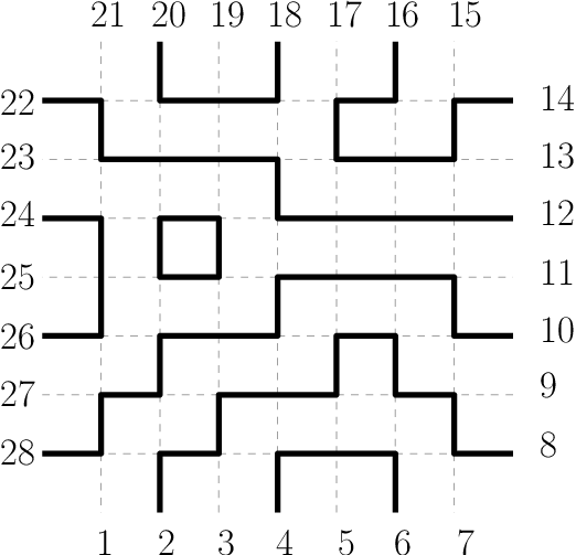
FPL configurations are known to be in bijection with numerous combinatorial objects, the most important being alternating sign matrices, whose enumeration was conjectured in [9], proved first by Zeilberger, and shortly after a shorter proof was given by Kuperberg:

In this work we will be interested by a refinement of FPLs, which is given by attaching to each configuration a link pattern which we now define.

We define a link pattern $X$ of size $n$ to be a noncrossing matching on $I$, where $I$ is any subset of the integers of cardinality $2n$. In other words, it is a partition of $I$ into pairs such that there are no integers $a<b<c<d$ such that $\{a,c\}$ and $\{b,d\}$ are both in $X$.

Now, since all vertices are of degree $2$ in an FPL configuration $F$, edges in $F$ are arranged in paths, which can be either closed or not, and in this last case both extremities of the paths are external edges. Therefore one can associate to $F$ a link pattern:

For instance, if $F$ is the configuration of Figure 2, then we have

We fix now a link pattern $X$ as in the previous definition and consider the rotated link pattern $r(X)$ defined by:

where indices are taken modulo $4n$. Note that $r$ corresponds geometrically to a counterclockwise rotation, and that it sends odd-labeled external edges to even-labeled ones and conversely. We have then the beautiful result of Wieland:

Now let $F$ be a configuration in $\mathcal{A}_{X}$, and let $c$ be any of its cells. We distinguish two cases: if there are precisely two edges of $F$ on opposite sides of $c$ (either horizontal or vertical), we define $U(c)=c$. Otherwise, we define $U(c)$ as the same cell where we exchange edges of $F$ and those that do not belong to $F$. Now, given $F$, apply $U$ to all active cells of $F$, and let the result be $W(F)$; note that the order in which $U$ is applied on active cells is irrelevant since any two of these cells share no edge. An illustration of the bijection is provided on Figure 5.

It is shown in [16] that $W$ is a bijection from $\mathcal{A}_{X}$ to $\mathcal{A}_{r(X)}$, and the reciprocal construction $W^{-1}$ consists in applying $U$ to cells which are not active.

$\square~$

This result has a nice consequence for enumeration, since one can rotate a link pattern to get a more pleasant, but equivalent counting problem: this technique is applied in [2, 3, 5]. Furthermore, we will make use of it in Section 2.1 as already mentioned, and it is at the heart of the proof of the Razumov–Stroganov conjecture in [1].

We consider finite words on the alphabet $\{0,1\}$, which we call $01$-words. For $u$ a $01$-word, we let $|u|_{0}$ denote the number of $0$s it contains, $|u|_{1}$ the number of $1$s it contains, and $|u|=|u|_{0}+|u|_{1}$ its total number of letters.

We need to define several notions for words, most of them coming from the Ferrers diagram representation.

We define the conjugate $\sigma^{*}$ of $\sigma=\sigma_{1}\cdots\sigma_{n}$ by $\sigma^{*}_{i}:=1-\sigma_{n+1-i}$; in the example of Figure 6 we get $\sigma^{*}=1000010101$. This corresponds to reflecting a Ferrers diagram with respect to its main diagonal. The inversion number of $\sigma$ is the number of indices $i<j$ such that $(\sigma_{i},\sigma_{j})=(1,0)$, and is noted $d(\sigma)$; this is the number of boxes in the Ferrers diagram representation. For instance we have $d(\sigma)=9$ for the example of Figure 6.

Now suppose $\sigma,\tau$ verify $|\sigma|_{0}=|\tau|_{0}$ and $|\sigma|_{1}=|\tau|_{1}$, so that they form Ferrers diagrams included in a common rectangle. We define a partial order by $\sigma\leq\tau$ if $\sigma$ is included in $\tau$ in the diagram representation. Define the partial sum $\sigma_{\leq i}=\sum_{j\leq i}\sigma_{j}$ (which is just the number of $1$s with index less or equal to $j$). Then it is easily seen that $\sigma\leq\tau$ if and only if $\sigma_{\leq i}\leq\tau_{\leq i}$ for all indices $i$.

We now define more notions related to diagrams: if $\sigma\leq\tau$, we define $\tau/\sigma$ as the set of boxes that are in $\tau$ but not in $\sigma$; if there are no two boxes in the same column (respectively row) of $\tau/\sigma$, then $\tau/\sigma$ is a horizontal strip (resp. vertical strip), and we write $\sigma\to\tau$. The size $d(\tau/\sigma)$ of a skew shape is naturally $d(\tau)-d(\sigma)$.

We define a semistandard Young tableau of shape $\sigma$ of length $N\geq 0$ to be a sequence $(\sigma^{(i)})_{i=0\ldots N}$ of words, where $\sigma^{(0)}=\mathbf{0}_{n}\leq\sigma^{(1)}\ldots\leq\sigma^{(N)}=\sigma$ and $\sigma^{(i+1)}/\sigma^{(i)}$ is a horizontal strip for all $i<N$. This is equivalent to the following usual definition: a filling of the boxes of the diagram $\sigma$ by positive integers not bigger than $N$, which are nondecreasing in each row from left to right, and increasing in each column from top to bottom.

Suppose that $u$ is a box in the diagram $\sigma$, which is in the $k$th row from the top and $d$th column from the left. The content $c(u)$ of $u$ is defined as $d-k$, while its hook-length $h(u)$ is defined as the number of boxes in $\sigma$ which are below $u$ and in the same column, or right of $u$ and in the same row ($u$ itself being counted just once). We have then:

We define $SSYT(\sigma,N)$ as this quantity considered as a polynomial in $N$. It has leading term $\frac{1}{H(\sigma)}N^{d(\sigma)}$ where $H(\sigma):=\prod_{u\in\sigma}{h(u)}$.

We will be particularly interested in the following set of words:

This is simply the set of well parenthesized words of length $2n$, known as Dyck words, which are counted by the Catalan number $|\mathcal{D}_{n}|=C_{n}:=\frac{1}{n+1}\binom{2n}{n}$.

Note that $(\mathcal{D}_{n},\leq)$ is a poset, with smallest element $\mathbf{0}_{n}:=0^{n}1^{n}$ and greatest element $\mathbf{1}_{n}:=(01)^{n}$; they are respectively the empty diagram and the diagram $\delta_{n}$, and the poset is isomorphic to an interval in Young’s lattice.

Suppose we have a non crossing matching $\pi$ on $\{1,\ldots,2n\}$, and a nonnegative integer $m$. We first consider the matching

that is, we add $m$ nested arches around the matching $\pi$. Now we fix an extra integer $k\geq 0$, and consider the link pattern $X(\pi,m,k)$ on the grid $G_{n+m}$ defined as follows: $k+2i-1$ and $k+2j-1$ are matched in $X(\pi,m,k)$ if and only if $i$ and $j$ are matched in $\pi_{(m)}$, where indices on the grid are taken modulo $4(n+m)$. An example of $X(\pi,m,k)$ is given on Figure 8.

Now an immediate consequence of Wieland’s rotation (Theorem 1.5) is that: for any $\pi,m,k$ as above, $A_{X(\pi,m,k+1)}=A_{X(\pi,m,k)}$. So this value is independent of $k$, and we can thus define the following:

Note that in particular we have $A_{\pi}(0)=A_{X}$ where $X=X(\pi,0,0)$ can be any link pattern, so that studying the $A_{\pi}(m)$ is equivalent to studying the $A_{X}$.

We assume from now on and until Theorem 2.7 that we have the inequality $m\geq 3n+k-1$: this condition ensures that all external edges corresponding to $\pi$ appear on the bottom boundary of the grid $G_{n+m}$.

This condition is verified on Figure 9. Note that numerous edges inside the grid are already drawn on the picture. The reason is that all these edges are part of all FPL configurations with link pattern $X(\pi,m,k)$: they are said to be fixed with respect to the link pattern. The basic lemma to prove that these edges are fixed is due to de Gier [4, Lemma 39]; how one applies this lemma in our case is done in detail in [3] and [15], so we will not repeat this here.

These fixed edges give rise to various regions in the grid: two of them are pentagons which we note $\mathcal{R}_{1}$ and $\mathcal{R}_{2}$, which are both adjacent to a third region $\mathcal{T}$ with a triangular shape. For this last region, we will sometimes write it as $\mathcal{T}^{n}$ to stress the dependence in $n$, and as $\mathcal{T}^{\pi}$ to indicate that a particular matching $\pi$ has been chosen on it bottom boundary; note also that $\mathcal{R}_{1}$ depends on $k$ and $n$, while $\mathcal{R}_{2}$ depends on $k,m$ and $n$. The rest of the grid is completely determined outside of these three regions, since all vertices there already have two incident fixed edges. The border between the region $\mathcal{R}_{1}$ and $\mathcal{T}$ (respectively $\mathcal{R}_{2}$ and $\mathcal{T}$) is indicated by a segment denoted $S_{1}$ (resp. $S_{2}$). These two segments cross precisely $2n$ vertical edges of the grid $G_{n+m}$, which we will write $v_{1},\ldots,v_{2n}$ from bottom to top for $S_{1}$, and $w_{1},\ldots,w_{2n}$ from top to bottom for $S_{2}$.

Note that $\sigma$ and $\tau$ have asymmetric interpretations, and that in [15, 18], other conventions are taken. Now we have the following crucial result:

Fix now $\sigma$ and $\tau$ in $\mathcal{D}_{n}$. We let $\mathcal{R}_{1}(\sigma,k)$ and $\mathcal{R}_{2}(\tau,m-3n-k+1)$ be the sets of fillings of the regions $\mathcal{R}_{1}$ and $\mathcal{R}_{2}$ that may arise as parts of FPL configurations $F$ verifying $X(\pi,m,k)$ and such that $\sigma=\sigma(F)$ and $\tau=\tau(F)$ respectively. By reflecting $\mathcal{R}_{2}$ vertically, we see that $\mathcal{R}_{2}(\tau,m-3n-k+1)$ is the same region as $\mathcal{R}_{1}(\tau^{*},m-3n-k+1)$, so we need only focus on $\mathcal{R}_{1}$.

As a preliminary step, extend the pentagonal region $\mathcal{R}_{1}$ by zigzag paths on the left to transform it in a (tilted) rectangular region; let $S^{0},S^{1},\ldots,S^{n+k}=S_{1}$ be the segments parallel to $S_{1}$ that divide the region, from the top left to the bottom right: see the left part of Figure 10. Let us now fix a filling $f$ in $\mathcal{R}_{1}(\sigma,k)$: we encode the vertical edges from $f$ which cross the segment $S^{i}$ by a word $\sigma^{i}$ of length $2n$, as we did for $\sigma(F)$ in Definition 2.2: that is, these vertical edges correspond to $0$ while the other ones correspond to $1$. Then we have in fact $\sigma^{i}\in\mathcal{D}_{n}$ for all $i$, and the sequence $\mathbf{0}_{n}=\sigma^{0}\leq\sigma^{1}\leq\ldots\sigma^{n+k}=\sigma$ is the desired semistandard tableau of shape $\sigma$ and length $n+k$.

$\square~$

On Figure 10 we obtain thus the following tableau:

which can be represented compactly by the tableau on the right.

With the help of the bijection of Proposition 2.4 and Figure 10, we can identify fillings in $\mathcal{R}_{1}(\sigma,k)$ with tableaux of shape $\sigma$ and length $n+k$ for $\sigma\in\mathcal{D}_{n}$. We use this to give a diagram representing the decomposition of $A_{\pi}(m)$ in a compact manner on Figure 11.

Now we consider the configurations in the triangle with left and right boundaries $\sigma$ and $\tau$ respectively, and bottom boundary $\pi$; we need to specify what constraints induced by the boundaries these configurations must obey. The choice of such boundaries correspond in fact to a certain link pattern on the external edges of the triangle, as pictured on the right of Figure 12. More precisely:

• •

  The $n$ occurrences of $1$ in the word $\sigma$ correspond to starting points of paths crossing the triangle, whose ending points correspond to the $n$ occurrences of $0$ in $\tau$.

• •

  The $n$ paths whose extremities are the lower external edges obey the matching $\pi$.

• •

  There may be closed paths inside the triangle.

Note that among the $n$ paths joining the left and right boundaries, the top path is reduced to a single vertex.

As is summarized by Figure 11, we can express the results from this section up to now as follows:

This proposition was stated for $k=0$ in [3], and in general in [15]. We can now state one of the main results of [3] (which answered [19, Conjecture 6]).

From Theorem 4.3(a) below, we know that nonzero terms in (2.2) occur only for $\sigma\leq\pi$, and by the remark following Theorem 1.7 we have that $\operatorname{SSYT}(\sigma,m-2n+1)$ has degree $d(\sigma)$ in $m$; therefore the polynomial $A_{\pi}(m)$ has degree at most $d(\pi)$. The coefficient in degree $d(\pi)$ is obtained when $\sigma=\pi$, which implies $\tau=\mathbf{0}_{n}$ by Theorem 4.3(b), and is thus given by

which achieves the proof.

$\square~$

In Sections 3 and 4, we will study the numbers ${t_{\sigma,\tau}^{\pi}}$ of TFPL configurations.

The next result was first stated as Conjecture 3.4 in [15]. It is another property of the numbers ${t_{\sigma,\tau}^{\pi}}$, but of a different flavor than the ones in Section 4 since it involves a relation between several of these numbers.

Indeed the l.h.s. of (3.1) counts configurations in a “left extended” triangle, and the r.h.s. counts configurations in a “right extended” triangle, both with boundaries $\sigma,\tau,\pi$. We will prove the result by showing that configurations counted by each member are in bijection.

We fix first $k,m>0$ integers such that $m>3n+k-1$, as well as semistandard Young tableaux $P$ of shape $\sigma$ and length $n+k$, and a tableau $Q$ of shape $\tau^{*}$ and length $m-2n-k$. Such tableaux exist if $k$ is chosen big enough, which we also suppose.

Now let $f$ be a left-extended TFPL configuration with boundaries $\sigma,\tau,\pi$. By the bijection of Proposition 2.6, $f,P$ and $Q$ define a certain FPL configuration $F$ on the grid $G_{n+m}$, with link pattern $X(\pi,m,k)$; see Figure 13, left.

We now apply Wieland’s rotation $W^{-1}$ to $F$ (cf. Theorem 1.5), and we obtain a certain FPL configuration $F^{\prime}$ with link pattern $X(\pi,m,k-1)$. By Proposition 2.6 again, this is equivalent to the data of a right extended TFPL configuration $f^{\prime}$ with left and right boundaries $\sigma^{\prime}$ and $\tau^{\prime}$, together with two tableaux $P^{\prime},Q^{\prime}$ of respective lengths $n+k,m-2n-k$, and respective shapes $\sigma^{\prime},\tau^{\prime}$. We can represent this in the diagram:

The following lemma shows that the action of Wieland’s rotation in the pentagonal regions is essentially trivial.

This covers all possible cases of edges attached to the marked vertex, and in each case we have that $v_{1}$ belongs to $F$ if and only if $v_{2}$ belongs to $F^{\prime}$. Therefore $P=P^{\prime}$ and their shapes $\sigma$ and $\sigma^{\prime}$ coincide, which achieves the proof of the lemma.

$\square~$

We can now finish the proof of Theorem 3.1: by the previous lemma, $\sigma^{\prime}=\sigma$ and $\tau^{\prime}=\tau$. Therefore the restriction of $W^{-1}$ to left-extended triangles gives the wanted bijection with the right extended triangles preserving the boundary conditions, which proves bijectively the relation (3.1).

$\square~$

We follow here the main ideas of [15], by expressing some of the results in the matrix language. All matrices will have rows and columns indexed by $D_{n}$ (with a given linear order). We also consider such matrices as linear endomorphisms of the vector space $\mathbb{C}\mathcal{D}_{n}$ of formal complex linear combinations of elements of $\mathcal{D}_{n}$, by setting $g(\tau):=\sum_{\sigma}g_{\sigma\tau}\tau$ for any matrix $g$.

Now if $k$ such that $0\leq k\leq m-3n+1$, Equation (2.1) can be rewritten:

and this can be visualized also on Figure 11. Also, the result of Theorem 3.1 is equivalent to:

which is in fact the way it is formulated in [15, Conjecture 3.4]. Thanks to repeated uses of the relation (3.3), we can push $t^{\pi}$ to the right in (3.2) to get

Now the expression for $A_{\pi}(m)$ above²² 2 let us note that this expression can be deduced from the FPL configuration by using Wieland’s rotation. Indeed, when $k$ becomes greater than $m-3n+1$, the triangle $\mathcal{T}^{n}$ gets more and more truncated by the right border of the grid, up until $k=m-2n+1$ where the truncated triangle is equivalent to a triangle ${\mathcal{T}_{\sigma,\tau}^{\pi}}$ with $\tau=\mathbf{0}_{n}$, and we get the formula. is polynomial in $m$ and we can in fact write the following proposition:

The passage from $\mathbf{t}$ to $\mathbf{t}^{\pi}$ is validated by the fact that $\left(\mathbf{t}^{\pi}\right)_{\sigma\mathbf{0}_{n}}=\left(\mathbf{t}\right)_{\sigma\pi}$ by definition. By Theorem 4.3 the coefficients $\left(\mathbf{t}\right)_{\sigma\pi}=t_{\sigma,\mathbf{0}_{n}}^{\pi}$ are integers, equal to $0$ unless $\sigma\leq\pi$, and such that $\left(\mathbf{t}\right)_{\pi\pi}=1$. This means that, if we give the basis $\mathcal{D}_{n}$ a linear order extending $\leq$, then the matrix of $\mathbf{t}$ becomes upper triangular with ones on its diagonal; it is thus invertible with inverse $\mathbf{t}^{-1}$ being also triangular with ones on its diagonal, and has integer entries.

We can now state the result conjectured³³ 3 Thapper shows in fact that the result is a consequence of the conjectural relations $\mathbf{b}\mathbf{t}_{*\tau}=\mathbf{t}_{*\tau}\mathbf{c}$ for any $\tau$, where $\left(\mathbf{t}_{*\tau}\right)_{\sigma\pi}={t_{\sigma,\tau}^{\pi}}.$ We show here that one can obtain the result without the help of these relations. by Thapper [15, Proposition 3.5]:

from which the result follows, again by Proposition 3.5.

$\square~$

Note that the fact there exist such coefficients is not in itself surprising: $A_{\pi}(m)$ has degree $d(\pi)\leq n(n-1)/2$ in $m$, and Theorem 3.7 expresses it as a linear combination of many more polynomials in general Furthermore such coefficients are in fact not unique as can be easily checked on examples.

What makes these coefficients interesting is the following: first, we have an explicit definition for them (even though it is not immediate to extract a lot of information from it). Then, a look at the data shows a lot of (mostly conjectural) properties for them, which lead then to new conjectures by Theorem 3.7: an example of this are the Conjectures 3.9 and 3.10 below.

The definition of $\mathbf{c}$ can be rewritten in the following equations for the coefficients $c_{\alpha\pi}$:

These relations clearly characterize completely the coefficients $c_{\alpha\pi}$, and we illustrate this by computing some of these coefficients:

If $\pi/\alpha$ has two disconnected cells, say a first one in column $h+1$ and a second one in column $h^{\prime}+1$ with $h^{\prime}>h$, then let $\pi_{1}$ (resp. $\pi_{2}$) denote the element of $\mathcal{D}_{n}$ obtained by adding the first cell (resp. the second one) to $\alpha$. Then the recurrence formula gives

Now from the case of one cell we have $c_{\pi_{1}\pi}=c_{\pi_{2}\pi}=1$, while $t_{\alpha}^{\pi_{1}}=t_{\pi_{2}}^{\pi}$, $t_{\alpha}^{\pi_{2}}=t_{\pi_{1}}^{\pi}$ follow from Corollary 4.9. The only remaining term after the simplifications is then $t_{\pi}^{\pi}=1$.

$(2)$ Let $\pi_{0}=\alpha<\pi_{1}<\ldots<\pi_{a-1}<\pi_{a}=\pi$ denote the shapes between $\alpha$ and $\pi$. Define also $X=2n-2-h$, where $h+1$ is the column of the cell $\pi_{1}/\alpha$.

$\bullet$ If $\pi/\alpha$ consists of cells in the same column, the result holds for $a=2$, since one gets

For $a>2$, only $\pi_{1}$ appears in the first sum in Equation 3.4; by induction on $a$, it simplifies to

the two quantities being equal by Corollary 4.9.

$\bullet$ If cells are in the same row, one has for the case $a=2$:

and proceeding by induction on $a$, Equation (3.4) becomes

where here also we used Corollary 4.9.

$\square~$

An interesting conjecture from [15] claims that $c_{\alpha\mathbf{1}_{n}}=1$ for all $\alpha\in\mathcal{D}_{n}$; by Theorem 3.7, this implies the following polynomial identity:

This last equality was conjectured by Wieland [16], and is now a theorem thanks to the Razumov–Stroganov correspondence [1] and Equation (4.8) in [6].

We conjecture the following special values for $c_{\alpha\pi}$:

When $\ell=0$ this reduces to Thapper’s conjecture that $c_{\alpha\mathbf{1}_{n}}=1$ for any $\alpha\in\mathcal{D}_{n}$.
By Theorem 3.7, the truth of Conjecture 3.9 implies a certain relation between FPLs on the square grid. To express this relation, we represent the numbers $A_{X}$ for a link pattern $X$ by using the chord diagram notation. The conjecture we obtain is the following:

This has been checked for all $i+j+\ell\leq 9$ and any $m$ by Tiago Fonseca (personal communication).

We fix coordinates on the triangle $\mathcal{T}^{n}$, by letting the origin be the bottom left vertex of the triangle, and take as basis vectors $(1,0)$ and $(0,1)$. The vertices of $\mathcal{T}^{n}$ are the points of coordinates $(x,y)\in\mathbb{Z}^{2}$ which verify $x\geq y\geq 0$ and $x+y\leq 4n-2$. Such vertices can be partitioned in lines: for $i\in\{1,\ldots,2n\}$, we define $E_{i}$ as the vertices of $\mathcal{T}^{n}$ such that $x+y=2i-2$, and for $i\in\{1,\ldots,2n-1\}$, we define $O_{i}$ as the vertices of $\mathcal{T}^{n}$ such that $x+y=2i-1$. The case $n=3$ is illustrated on Figure 14.

Now let us suppose we have boundary configurations $\sigma,\tau,\pi$ in $\mathcal{D}_{n}$. We define an orientation for all edges around the triangle as follows. On the left boundary, we orient edges to the right and upwards; on the right boundary, we orient them to the right and downwards. Finally, for the $2n$ vertical external edges on the bottom, we orient the one attached to $(2i-2,0)$ upwards if $\pi_{i}=0$, and downwards if $\pi_{i}=1$, for $i\in\{1,\ldots,2n\}$.

References

- [1] Luigi Cantini and Andrea Sportiello. Proof of the Razumov-Stroganov conjecture. J. Combin. Theory Ser. A, 118(5):1549–1574, 2011.
- [2] F. Caselli and C. Krattenthaler. Proof of two conjectures of Zuber on fully packed loop configurations. J. Combin. Theory Ser. A, 108(1):123–146, 2004.
- [3] F. Caselli, C. Krattenthaler, B. Lass, and P. Nadeau. On the number of fully packed loop configurations with a fixed associated matching. Electron. J. Combin., 11(2):Research paper 16, 2004.
- [4] J. de Gier. Loops, matchings and alternating-sign matrices. Discrete Math., 298(1-3):365–388, 2005.
- [5] P. Di Francesco and J.-B. Zuber. On fully packed loop configurations with four sets of nested arches. J. Stat. Mech. Theory Exp., (6):005, 20 pp. (electronic), 2004.
- [6] T. Fonseca and P. Zinn-Justin. On some ground state components of the O(1) loop model. Journal of Statistical Mechanics: Theory and Experiment, 2009(03):P03025 (29pp), 2009.
- [7] I. Gessel and G. Viennot. Binomial determinants, paths, and hook length formulae. Adv. in Math., 58(3):300–321, 1985.
- [8] G. Kuperberg. Another proof of the alternating-sign matrix conjecture. Internat. Math. Res. Notices, (3):139–150, 1996.
- [9] W. Mills, D. Robbins, and Jr. H. Rumsey. Proof of the Macdonald conjecture. Invent. Math., 66(1):73–87, 1982.
- [10] P. Nadeau. Fully Packed Loop configurations in a triangle II. Littlewood Richardson coefficients. in preparation.
- [11] P. Nadeau. Fully Packed Loop configurations in a triangle and Littlewood–Richardson coefficients. DMTCS Proceedings, 0(01), 2010.
- [12] J. Propp. The many faces of alternating-sign matrices, 2001.
- [13] A. Razumov and Yu. Stroganov. Combinatorial nature of the ground-state vector of the loop model. Teoret. Mat. Fiz., 138(3):395–400, 2004.
- [14] R. P. Stanley. Theory and application of plane partitions. I, II. Studies in Appl. Math., 50:167–188; ibid. 50 (1971), 259–279, 1971.
- [15] J. Thapper. Refined counting of fully packed loop configurations. Séminaire Lotharingien de Combinatoire, 56:B56e, 2007.
- [16] B. Wieland. A large dihedral symmetry of the set of alternating sign matrices. Electron. J. Combin., 7:Research Paper 37, 13 pp, 2000.
- [17] D. Zeilberger. Proof of the alternating sign matrix conjecture. Electron. J. Combin., 3(2):Research Paper 13, 84 pp, 1996. The Foata Festschrift.
- [18] P. Zinn-Justin. A conjectured formula for fully packed loop configurations in a triangle. Electron. J. Combin., 17(1):Research Paper 107, 2010. arXiv:0911.4617v1.
- [19] J.-B. Zuber. On the Counting of Fully Packed Loop Configurations: Some new conjectures. Electron. J. Combin., 11(1):Research paper 13, 2004.