We solve the gaugino Dirac equation on a smeared intersecting five-brane solution in $E_{8}~\times~E_{8}$ heterotic string theory to search for localized chiral zeromodes on the intersection. The background is chosen to depend on the full two-dimensional overall transverse coordinates to the branes. Under some appropriate boundary conditions, we compute the complete spectrum of zeromodes to find that, among infinite towers of Fourier modes, there exist only three localized normalizable zeromodes, one of which has opposite chirality to the other two. This agrees with the result previously obtained in the domain-wall type solution, supporting the claim that there exists one net chiral zeromode localized on the heterotic five-brane system.

November 2011

Flux compactifications of string theory on non-Kähler manifolds [1]-[21] have attracted much interest for some recent years. In heterotic string theory, it has been known for a long time that the moduli are partially stabilized by the NS-NS three form flux $H_{MNP}$[1][2][3]. In general, turning on fluxes produces a potential [4], and one finds new vacua with some stabilized moduli at the potential minima [5]-[11]. More recently, understanding of heterotic moduli stabilization was improved by taking into account the intrinsic torsion of the geometry [12]-[21].

Historically, heterotic string theory was extensively studied in 1980s as a candidate unified theory including gravity. After the D-branes were found, however, the research focus has shifted from heterotic to type II theories, in particular, while the brane-world scenario [22] [23] was readily realized in type II theories using D-branes, there are no known such constructions in heterotic string theory. Despite this, an attempt was made in [24] to realize warped compactification of heterotic string theory by using NS5-branes, where the authors considered a domain-wall type smeared intersecting NS5-brane solution in $E_{8}~{\times}~E_{8}$ heterotic string theory and explicitly solved the gaugino Dirac equation to find one net chiral fermionic zeromode. This result was in agreement with the naive counting argument of Nambu-Goldstone modes on this background [24].

In this paper, we perform the gaugino-zeromode analysis on a similar smeared intersecting background, in which, unlike the one considered in [24], the field configurations depend on not only just one of the overall transverse coordinates (that is, the domain-wall type) but full two-dimensional overall transverse coordinates to the branes (the vortex type) ¹¹ 1 They constitute the intersecting $p$-brane solution in the original form obtained in [25, 26]. Note that the relatively transverse dimensions are still smeared. . Although the Dirac operator becomes nontrivial and much more complicated than the one considered in [24], we will solve the zeromode equation under some boundary conditions, and compute the complete spectrum of zeromodes. In particular, we will find that, among infinite towers of Fourier modes, there exist only three localized normalizable zeromodes, one of which has opposite chirality to the other two. This agrees with the result obtained in [24], supporting the claim that there exists one net chiral zeromode localized on the intersection of the heterotic five-brane system.

We begin with the neutral smeared intersecting five-brane solution [25] [26]:

	$\displaystyle ds^{2}$	$\displaystyle=$	$\displaystyle\sum_{i,j=0,7,8,9}\eta_{ij}dx^{i}dx^{j}+h(x^{1},x^{2})^{2}\sum_{\mu,\nu=1,2}\delta_{\mu\nu}dx^{\mu}dx^{\nu}+h(x^{1},x^{2})\sum_{\mu,\nu=3,4,5,6}\delta_{\mu\nu}dx^{\mu}dx^{\nu},$
	$\displaystyle h(x^{1},x^{2})^{2}$	$\displaystyle=$	$\displaystyle e^{2\phi},$		(1)

where

$\displaystyle h(x^{1},x^{2})=h_{0}+\xi\log{r}~,~~r=\sqrt{(x^{1})^{2}+(x^{2})^{2}},$

(2)

$h_{0}$ and $\xi$ are real constants. The profiles of the harmonic function $h(x^{1},x^{2})$ are shown in Figure 2 for $\xi<0$, and in Figure 2 for $\xi>0$.

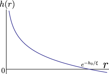
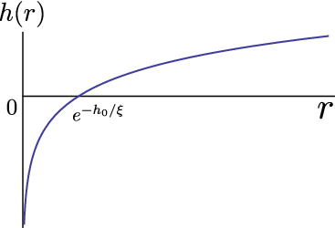
Since $h(x^{1},x^{2})$ is equal to the string coupling, we only consider the region where $h(x^{1},x^{2})$ is positive, and impose the boundary condition that all the fields become $0$ where $h=0$. The 3-form flux $H_{\mu\nu\rho}$ is

$\displaystyle H_{\mu\nu\rho}=\begin{cases}{1\over 2}{\partial h(x^{1},x^{2})\over\partial x^{1}}&\mbox{if $(\mu,\nu,\rho)=(2,3,4),(2,5,6)$ and even permutations},\\ -{1\over 2}{\partial h(x^{1},x^{2})\over\partial x^{1}}&\mbox{if $(\mu,\nu,\rho)=(2,4,3),(2,6,5)$ and even permutations},\\ -{1\over 2}{\partial h(x^{1},x^{2})\over\partial x^{2}}&\mbox{if $(\mu,\nu,\rho)=(1,3,4),(1,5,6)$ and even permutations},\\ {1\over 2}{\partial h(x^{1},x^{2})\over\partial x^{2}}&\mbox{if $(\mu,\nu,\rho)=(1,4,3),(1,6,5)$ and even permutations},\\ 0&\mbox{otherwise}.\end{cases}$

(3)

(1) and (3) are a solution to the equations of motion of the type II NS-NS sector Lagrangian. The metric (1) represents two NS5-branes extended in the dimensions shown in Table 1. We emphasize here that our solution is different from the one adopted in [24] in that the harmonic function (2) has a dependence on both the $x^{1}$ and $x^{2}$ coordinates.

In (2), the parameter $\xi$ is related to the NS5-brane tension. The brane action is calculated by using the equations of motion as follows (in the Einstein frame):

$\displaystyle S_{\mbox{\tiny 5-Brane1}}=-{T\over 2\kappa^{2}}\int d^{6}x\sqrt{-\det{G_{mn}}}e^{-\phi/2}\delta(x^{1},x^{2}),$

where $G_{mn}$ is the six-dimensional metric $(m,n=0,5,6,7,8,9)$, and $T$ is the brane tension

$\displaystyle T=-2\pi\xi.$

Therefore, if $\xi<0$, the 5-brane tension is positive. On the other hand, if $\xi>0$, the tension becomes negative, implying that this is an orientifold-like object. In [28], it was argued that such an object in heterotic string theory might be understood as a mirror to the Atiyah-Hitchin manifold. In this paper, we only study positive tension branes.

Next we convert this type II NS5-brane background into an $E_{8}~{\times}~E_{8}$ heterotic background by the standard embedding [29]. We generalize the spin connection $\omega_{\mu}$ by adding the 3-form flux $H_{\mu\nu\rho}$

$\displaystyle\Omega_{\pm\mu}^{~\alpha\beta}=\omega_{\mu}^{~\alpha\beta}\pm H_{\mu}^{~\alpha\beta},$

(4)

and we identify $\Omega_{+\mu}$ to the gauge connection $A_{\mu}$. We present the gauge connections using Gell-Mann matrices $\lambda_{i}$ $(i=1,{\cdots},8)$ and $2{\times}2$ matrices $\mbox{\boldmath$1$}\equiv\left(\begin{array}[]{cc}1&0\\ 0&1\end{array}\right)$, $\mbox{\boldmath$s$}\equiv i\sigma_{2}=\left(\begin{array}[]{cc}0&1\\ -1&0\end{array}\right)$:

	$\displaystyle A_{1}^{~\alpha\beta}$	$\displaystyle=$	$\displaystyle-{1\over h(x^{1},x^{2})}{\partial h(x^{1},x^{2})\over\partial x^{2}}\{-{3\over 4}(3\lambda_{3}+\sqrt{3}\lambda_{8})\}~{\otimes}~\mbox{\boldmath$s$},$		(5)
	$\displaystyle A_{2}^{~\alpha\beta}$	$\displaystyle=$	$\displaystyle{1\over h(x^{1},x^{2})}{\partial h(x^{1},x^{2})\over\partial x^{1}}\{-{3\over 4}(3\lambda_{3}+\sqrt{3}\lambda_{8})\}~{\otimes}~\mbox{\boldmath$s$},$
	$\displaystyle A_{3}^{~\alpha\beta}$	$\displaystyle=$	$\displaystyle{1\over 2h(x^{1},x^{2})^{3/2}}{\partial h(x^{1},x^{2})\over\partial x^{1}}(-i\lambda_{2})~{\otimes}~\mbox{\boldmath$1$ }-{1\over 2h(x^{1},x^{2})^{3/2}}{\partial h(x^{1},x^{2})\over\partial x^{2}}(-\lambda_{1})~{\otimes}~\mbox{\boldmath$s$},$
	$\displaystyle A_{4}^{~\alpha\beta}$	$\displaystyle=$	$\displaystyle{1\over 2h(x^{1},x^{2})^{3/2}}{\partial h(x^{1},x^{2})\over\partial x^{1}}(-\lambda_{1})~{\otimes}~\mbox{\boldmath$s$ }+{1\over 2h(x^{1},x^{2})^{3/2}}{\partial h(x^{1},x^{2})\over\partial x^{2}}(-i\lambda_{2})~{\otimes}~\mbox{\boldmath$1$},$
	$\displaystyle A_{5}^{~\alpha\beta}$	$\displaystyle=$	$\displaystyle{1\over 2h(x^{1},x^{2})^{3/2}}{\partial h(x^{1},x^{2})\over\partial x^{1}}(-i\lambda_{5})~{\otimes}~\mbox{\boldmath$1$ }+{1\over 2h(x^{1},x^{2})^{3/2}}{\partial h(x^{1},x^{2})\over\partial x^{2}}(+\lambda_{4})~{\otimes}~\mbox{\boldmath$s$},$
	$\displaystyle A_{6}^{~\alpha\beta}$	$\displaystyle=$	$\displaystyle-{1\over 2h(x^{1},x^{2})^{3/2}}{\partial h(x^{1},x^{2})\over\partial x^{1}}(+\lambda_{4})~{\otimes}~\mbox{\boldmath$s$ }-{1\over 2h(x^{1},x^{2})^{3/2}}{\partial h(x^{1},x^{2})\over\partial x^{2}}(-i\lambda_{5})~{\otimes}~\mbox{\boldmath$1$}.$

$\Omega_{+\mu}$, which is generically an $SO(6)$ spin connection, can be written in this form and set equal to the gauge connection $A_{\mu}$, thanks to the $SU(3)$ structure of this background. The eigenvalues of $s$, $\pm i$, distinguish which $SU(3)$ representation the gaugino is in, $3$ or $\bar{\mbox{\boldmath$3$}}$. We adopt $\mbox{\boldmath$s$}=+i$ from now on. These backgrounds (3) and (5) preserve 1/4 of supersymmetries since the generalized spin connections $\Omega_{\pm\mu}$ are in $SU(3)$. In order to satisfy the Bianchi identity $dH=0$, we embed the gauge group $SU(3)$ to $E_{8}~{\times}~E_{8}$ and get the unbroken gauge symmetry $E_{6}(\times E_{8})$. The adjoint representation of $E_{8}$ is decomposed by embedding $SU(3)$ as follows:

$\displaystyle\mbox{\boldmath$248$}=(\mbox{\boldmath$78$},\mbox{\boldmath$1$})~{\oplus}~(\mbox{\boldmath$27$},\mbox{\boldmath$3$})~{\oplus}~(\bar{\mbox{\boldmath$27$}},\bar{\mbox{\boldmath$3$}})~{\oplus}~(\mbox{\boldmath$1$},\mbox{\boldmath$8$}).$

(6)

Since the gauge field has a vev in $SU(3)$, the fields which are transformed as $(\mbox{\boldmath$27$},\mbox{\boldmath$3$})~{\oplus}~(\bar{\mbox{\boldmath$27$}},\bar{\mbox{\boldmath$3$}})$ (as well as $(\mbox{\boldmath$1$},\mbox{\boldmath$8$})$) become Nambu-Goldstone bosons. We know that a $D=4$, ${\cal N}=1$ chiral supermultiplet have only two bosonic degrees of freedom. The Nambu-Goldstone bosons, which belongs to $27$ and $\bar{\mbox{\boldmath$27$}}$, must be combined with their superpartners to a single ${\cal N}=1$ chiral supermultiplet. This means that the moduli are a triplet (of the broken $SU(3)$) of chiral supermultiplets that transform as $27$ (or $\bar{\mbox{\boldmath$27$}}$) of $E_{6}$. Therefore, from this bosonic moduli counting argument one might conclude that there would be three chiral zeromodes. In fact, however, there is left only one net generation of fermions on the intersecting NS5-brane since the chiralities of the localized solutions are different, as we show below. The results agree with [24].

To know the number of generations that localize on the branes, we need to compute the Dirac indices. The ten-dimensional heterotic gaugino equation of motion is

$\displaystyle\Gamma^{M}D_{M}(\omega-{1\over 3}H,A)\chi-\Gamma^{M}\chi\partial_{M}\phi+{1\over 8}\Gamma^{M}\gamma^{AB}(F_{AB}+\hat{F}_{AB})(\psi_{M}+{2\over 3}\Gamma_{M}\lambda)=0,$

(7)

where

$\displaystyle D_{M}(\omega-{1\over 3}H,A)\chi\equiv\Bigl(\partial_{M}+{1\over 4}(\omega_{M}^{~AB}-{1\over 3}H_{M}^{~AB})\gamma_{AB}+\mbox{ad}A_{M}\Bigr)\chi$

(8)

and $\mbox{ad}A_{M}{\cdot}\chi\equiv[A_{M},\chi]$. We set $\psi_{M}=0$, $\lambda=0$ and $\tilde{\chi}\equiv e^{-\phi}\chi$, the equation of motion becomes

$\displaystyle\Gamma^{M}D_{M}(\omega-{1\over 3}H,A)\tilde{\chi}=0.$

(9)

The $SO(9,1)$ gamma matrices $\Gamma^{M}$ are

$\displaystyle\Gamma^{a}=\gamma^{a}_{\mbox{\tiny 4D}}{\otimes}\mbox{\boldmath$1$}_{8},~~(a=0,7,8,9)~~~\Gamma^{\alpha}=\gamma^{\sharp}_{\mbox{\tiny 4D}}{\otimes}\gamma^{\alpha}~~(\alpha=1,{\dotsc},6)$

where $\gamma^{a}_{\mbox{\tiny 4D}}$, $\gamma^{\sharp}_{\mbox{\tiny 4D}}$ are the ordinary $SO(3,1)$ gamma matrices and chiral operator, respectively. $\gamma^{\alpha}$ are the $SO(6)$ gamma matrix and we fix them as

	$\displaystyle\gamma^{1}=\sigma_{1}{\otimes}\mbox{\boldmath$1$}{\otimes}\mbox{\boldmath$1$},~~\gamma^{2}=\sigma_{2}{\otimes}\mbox{\boldmath$1$}{\otimes}\mbox{\boldmath$1$},~~\gamma^{3}=\sigma_{3}{\otimes}\sigma_{1}{\otimes}\mbox{\boldmath$1$},$
	$\displaystyle\gamma^{4}=\sigma_{3}{\otimes}\sigma_{2}{\otimes}\mbox{\boldmath$1$},~~\gamma^{5}=\sigma_{3}{\otimes}\sigma_{3}{\otimes}\sigma_{1},~~\gamma^{6}=\sigma_{3}{\otimes}\sigma_{3}{\otimes}\sigma_{2}.$

The $SO(6)$ chiral operator is defined by $\gamma^{\sharp}=-i\gamma^{1}\gamma^{2}\gamma^{3}\gamma^{4}\gamma^{5}\gamma^{6}$. More explicitly, it is represented in the matrix form:

$\displaystyle\gamma^{\sharp}=\left(\begin{array}[]{cccccccc}-\mbox{\boldmath$1$}_{3}&0&0&0&0&0&0&0\\ 0&\mbox{\boldmath$1$}_{3}&0&0&0&0&0&0\\ 0&0&\mbox{\boldmath$1$}_{3}&0&0&0&0&0\\ 0&0&0&-\mbox{\boldmath$1$}_{3}&0&0&0&0\\ 0&0&0&0&\mbox{\boldmath$1$}_{3}&0&0&0\\ 0&0&0&0&0&-\mbox{\boldmath$1$}_{3}&0&0\\ 0&0&0&0&0&0&-\mbox{\boldmath$1$}_{3}&0\\ 0&0&0&0&0&0&0&\mbox{\boldmath$1$}_{3}\end{array}\right)$

where $\mbox{\boldmath$1$}_{3}=\left(\begin{array}[]{ccc}1&0&0\\ 0&1&0\\ 0&0&1\end{array}\right)$. We can decompose an $SO(9,1)$ Majorana-Weyl spinor into $SO(3,1)$ and $SO(6)$ spinors as $\mbox{\boldmath$16$}=(\mbox{\boldmath$2$}_{+},\mbox{\boldmath$4$}_{+})~{\oplus}~(\mbox{\boldmath$2$}_{-},\mbox{\boldmath$4$}_{-})$, where the subscripts $\pm$ are the $SO(3,1)$ and $SO(6)$ chiralities. Since the $SO(9,1)$ spinor is Majorana, the $(\mbox{\boldmath$2$}_{+},\mbox{\boldmath$4$}_{+})$ and $(\mbox{\boldmath$2$}_{-},\mbox{\boldmath$4$}_{-})$ components are associated with charge conjugation.

Equation (9) can be divided into $i=0,7,8,9$ and $\mu=1,{\cdots},6$ directions [30]

$\displaystyle\Gamma^{i}\partial_{i}\tilde{\chi}+\Gamma^{\mu}D_{\mu}(\omega-{1\over 3}H,A)\tilde{\chi}=0.$

(19)

If $\tilde{\chi}=\tilde{\chi}_{\mbox{\tiny 4D}}~{\otimes}~\tilde{\chi}_{\mbox{\tiny 6D}}$, the second term looks like the mass term of the four dimensional Dirac equation. Being a singular noncompact geometry, no index theorem is available on our background. Therefore, in order to count the number of localized fermionic zeromodes on the intersection of the five-branes we will solve the Dirac equation directly

$\displaystyle\gamma^{\mu}D_{\mu}(\omega-{1\over 3}H,A)\tilde{\chi}_{\mbox{\tiny 6D}}=0$

(20)

and find localized solutions which may have either positive or negative chirality.

The gauge connection $A_{\mu}$ has nonzero value in the $SU(3)$ subalgebra, and therefore the $\tilde{\chi}_{\mbox{\tiny 6D}}$ is transformed as a triplet of $SU(3)$. We know that the chiralities of $\tilde{\chi}_{\mbox{\tiny 6D}}$ related to each other by charge conjugation. If we change the representation of the $SU(3)$, $3$ or $\bar{\mbox{\boldmath$3$}}$, the chirality of $\tilde{\chi}_{\mbox{\tiny 6D}}$ also changes oppositely. Since $\tilde{\chi}_{\mbox{\tiny 6D}}$ depend only $x^{1}$ and $x^{2}$, (20) becomes

$\displaystyle\left(\begin{array}[]{cc}&\partial_{\bar{z}}~\mbox{\boldmath$1$}_{12}\\ \partial_{z}~\mbox{\boldmath$1$}_{12}&\end{array}\right)\tilde{\chi}_{\mbox{\tiny 6D}}+{\cal{M}}\tilde{\chi}_{\mbox{\tiny 6D}}=0,$

where

	$\displaystyle\partial_{z}$	$\displaystyle=$	$\displaystyle{\partial\over\partial z}\equiv{\partial\over\partial x^{1}}+i{\partial\over\partial x^{2}},~~\partial_{\bar{z}}={\partial\over\partial\bar{z}}\equiv{\partial\over\partial x^{1}}-i{\partial\over\partial x^{2}},$
	$\displaystyle{\cal M}$	$\displaystyle=$	$\displaystyle\gamma^{\mu}\{{1\over 4}(\omega_{\mu}^{~AB}-{1\over 3}H_{\mu}^{~AB})\Gamma_{AB}+\mbox{ad}A_{\mu}\},$

and ${\mbox{\boldmath$1$}}_{12}$ is the $12{\times}12$ unit matrix. $\tilde{\chi}_{\mbox{\tiny 6D}}$ is a fermion that has 24 components, and we solve the Dirac equation (S0.EGx17) for each component. In order to find solutions, we expand these components by Fourier modes as

$\displaystyle\tilde{\chi}_{\mbox{\tiny 6D}}^{\pm N}=\sum_{m=-\infty}^{\infty}e^{im\theta}\tilde{\chi}_{\mbox{\tiny 6D}~m}^{\pm N}(r),$

(24)

where the signs $\pm$ denote the chiralities, and $N$ $(=1,{\cdots},12)$ label the components of the gaugino $\tilde{\chi}_{\mbox{\tiny 6D}}$. Thus we obtain 24 Dirac equations from (S0.EGx17) form each component, some of which are complicated differential equations. However, we can find a linear transformation matrix $T$ :

$\displaystyle T=\left(\begin{array}[]{cc}t_{1}&t_{2}\\ t_{2}&t_{1}\end{array}\right),$

$\displaystyle t_{1}=\left(\begin{array}[]{cccccccccccc}0&0&0&0&0&-1/2&0&-1/2&0&0&0&0\\ 0&0&0&0&0&0&0&0&0&0&0&0\\ 0&0&0&0&0&0&0&0&0&0&0&0\\ 0&0&0&1/2&0&0&0&0&0&0&0&0\\ 0&0&0&0&1&0&0&0&0&0&0&0\\ 0&0&0&0&0&1/2&0&-1/2&0&0&0&0\\ 0&0&0&0&0&0&1/2&0&0&0&0&0\\ 0&0&0&0&0&1/4&0&1/4&0&0&0&0\\ 0&0&0&0&0&0&0&0&1&0&0&0\\ 0&0&0&0&0&0&0&0&0&0&0&0\\ 0&0&0&1/2&0&0&0&0&0&0&0&0\\ 0&0&0&0&0&0&1/2&0&0&0&0&0\end{array}\right),$

$\displaystyle t_{2}=\left(\begin{array}[]{cccccccccccc}1/2&0&0&0&0&0&0&0&0&0&0&0\\ 0&1&0&0&0&0&0&0&0&0&0&0\\ 0&0&1&0&0&0&0&0&0&0&0&0\\ 0&0&0&0&0&0&0&0&0&0&-1/2&0\\ 0&0&0&0&0&0&0&0&0&0&0&0\\ 0&0&0&0&0&0&0&0&0&0&0&0\\ 0&0&0&0&0&0&0&0&0&0&0&-1/2\\ 1/2&0&0&0&0&0&0&0&0&0&0&0\\ 0&0&0&0&0&0&0&0&0&0&0&0\\ 0&0&0&0&0&0&0&0&0&1&0&0\\ 0&0&0&0&0&0&0&0&0&0&1/2&0\\ 0&0&0&0&0&0&0&0&0&0&0&1/2\end{array}\right).$

and define a new gaugino field $\tilde{\chi}^{\prime}_{\mbox{\tiny 6D}}=T\tilde{\chi}_{\mbox{\tiny 6D}}$. Then the equations in terms of the new components of $\tilde{\chi}^{\prime}_{\mbox{\tiny 6D}}$ become first order differential equations of the radial coordinate $r$, so that one can easily solve the equations.

The generic form of these 24 equations can be written as follows:

$\displaystyle{d\over dr}\tilde{\chi}_{\mbox{\tiny 6D}~m}^{\pm N}-{m+n(N)\over r}\tilde{\chi}_{\mbox{\tiny 6D}~m}^{\pm N}+{\alpha(N)\over h(r)^{2}}{dh(r)\over dr}\tilde{\chi}_{\mbox{\tiny 6D}~m}^{\pm N}=0,$

(54)

where $n(N)$ is an integer which depends on each $N$. The real numbers $\alpha(N)$ are found to be

	$\displaystyle+~:~~\alpha$	$\displaystyle=$	$\displaystyle\{~2~,~{3\over 2}~,~{3\over 2}~,~{3\over 2}~,~1~,~1~,~{7\over 2}~,~-1~,~1~,~1~,~{7\over 2}~,~{3\over 2}~\}$
	$\displaystyle-~:~~\alpha$	$\displaystyle=$	$\displaystyle\{~1~,~{3\over 2}~,~{3\over 2}~,~{3\over 2}~,~2~,~2~,~-{1\over 2}~,~4~,~2~,~2~,~-{1\over 2}~,~{3\over 2}~\}$		(55)

for each chirality. These sets of numbers are exactly the same as the ones encountered in the domain-wall type case [24]. Note, however, that, unlike [24], our equations (54) depends on the Fourier frequency $m$.

The solutions of (54), with a constant of integration $C$, are

$\displaystyle\tilde{\chi}_{\mbox{\tiny 6D}~m}^{\pm N}=Cr^{m+n(N)}e^{\alpha\over h(r)}.$

(56)

We consider the cases of $\alpha>0$ and $\alpha<0$ separately.

(i) $\alpha(N)>0$
In this case the boundary condition is satisfied if and only if $C=0$, and therefore there are no localized modes.

(ii) $\alpha(N)<0$
In this case, any Fourier mode satisfies the boundary condition. However, we also require that the mode must be normalizable $\int d^{2}x|\tilde{\chi}|^{2}<\infty$. Such modes are the ones with $m+n(N)=0$; only a single Fourier mode corresponds to a normalizable mode and is localized for each negative $\alpha(N)$.

Therefore, the sets (55) show that there is only one normalizable localized mode with positive chirality, while there are two with negative chirality. This is exactly the same result as [24], confirming the claim that there exists one net chiral zeromode localized on this heterotic five-brane system.

References

- [1] R. Rohm and E. Witten, Annals Phys. 170 (1986) 454.
- [2] A. Strominger, Nucl. Phys. B 274 (1986) 253.
- [3] M. Dine, R. Rohm, N. Seiberg and E. Witten, Phys. Lett. B 156 (1985) 55.
- [4] S. Gukov, C. Vafa and E. Witten, Nucl. Phys. B 584 (2000) 69 [Erratum-ibid. B 608 (2001) 477] [arXiv:hep-th/9906070].
- [5] S. Kachru, R. Kallosh, A. D. Linde and S. P. Trivedi, Phys. Rev. D 68 (2003) 046005 [arXiv:hep-th/0301240].
- [6] T. R. Taylor and C. Vafa, Phys. Lett. B 474 (2000) 130 [arXiv:hep-th/9912152].
- [7] G. Dall’Agata, JHEP 0111 (2001) 005 [arXiv:hep-th/0107264].
- [8] S. Ferrara and M. Porrati, Phys. Lett. B 545 (2002) 411 [arXiv:hep-th/0207135].
- [9] S. Kachru, M. B. Schulz, P. K. Tripathy and S. P. Trivedi, JHEP 0303 (2003) 061 [arXiv:hep-th/0211182].
- [10] K. Becker, M. Becker, P. S. Green, K. Dasgupta and E. Sharpe, Nucl. Phys. B 678 (2004) 19 [arXiv:hep-th/0310058].
- [11] J. P. Gauntlett, D. Martelli and D. Waldram, Phys. Rev. D 69 (2004) 086002 [arXiv:hep-th/0302158].
- [12] G. Lopes Cardoso, G. Curio, G. Dall’Agata, D. Lust, P. Manousselis and G. Zoupanos, Nucl. Phys. B 652 (2003) 5 [arXiv:hep-th/0211118].
- [13] K. Becker, M. Becker, K. Dasgupta and S. Prokushkin, Nucl. Phys. B 666 (2003) 144 [arXiv:hep-th/0304001].
- [14] G. Lopes Cardoso, G. Curio, G. Dall’Agata and D. Lust, JHEP 0310 (2003) 004 [arXiv:hep-th/0306088].
- [15] G. Lopes Cardoso, G. Curio, G. Dall’Agata and D. Lust, Fortsch. Phys. 52 (2004) 483 [arXiv:hep-th/0310021].
- [16] K. Becker, M. Becker, K. Dasgupta and P. S. Green, JHEP 0304 (2003) 007 [arXiv:hep-th/0301161].
- [17] G. Curio, A. Krause and D. Lust, Fortsch. Phys. 54 (2006) 225 [arXiv:hep-th/0502168].
- [18] S. Gukov, S. Kachru, X. Liu and L. McAllister, Phys. Rev. D 69 (2004) 086008 [arXiv:hep-th/0310159].
- [19] B. de Carlos, S. Gurrieri, A. Lukas and A. Micu, JHEP 0603 (2006) 005 [arXiv:hep-th/0507173].
- [20] M. Becker and K. Dasgupta, arXiv:hep-th/0312221.
- [21] M. Serone and M. Trapletti, JHEP 0401 (2004) 012 [arXiv:hep-th/0310245].
- [22] L. Randall, R. Sundrum, Phys. Rev. Lett. 83 (1999) 3370-3373.
- [23] L. Randall, R. Sundrum, Phys. Rev. Lett. 83 (1999) 4690-4693.
- [24]
T. Kimura, S. Mizoguchi,
JHEP 1004, (2010) 028.
[arXiv:0912.1334 [hep-th]].
T. Kimura, S. Mizoguchi, Class. Quant. Grav. 27, (2010) 185023. [arXiv:0905.2185 [hep-th]]. - [25] R. Argurio, F. Englert and L. Houart, Phys. Lett. B 398, (1997) 61 [arXiv:hep-th/9701042].
- [26] N. Ohta, Phys. Lett. B 403 (1997) 218 [arXiv:hep-th/9702164].
- [27] K. Ohta and T. Yokono, JHEP 0002 (2000) 023 [arXiv:hep-th/9912266].
- [28] H. Imazato, S. Mizoguchi and M. Yata, [arXiv:1107.3557 [hep-th]].
- [29] C. G. Callan, J. A. Harvey and A. Strominger, Nucl. Phys. B 359 (1991) 611.
- [30] T. Kimura and P. Yi, JHEP 0607 (2006) 030 [arXiv:hep-th/0605247].