Ground states of dipolar gases in quasi-1D ring traps

We consider a system of $N$ identical particles (bosons or fermions) of mass $m$, confined in a ring-shaped trapping potential. The ring (radius $R$) is taken to lie in the $xy$-plane (Fig. 1). The particles (e.g., atoms with a magnetic moment or polar molecules) have a dipole moment $\mathbf{d}=d\left(\sin\alpha,0,\cos\alpha\right)$ aligned in the $xz$-plane by an external field, at an angle $\alpha$ to the $z$-axis. The interaction between two dipoles in free space is $V(\mathbf{r})=D^{2}(1-3\cos^{2}\theta_{rd})/r^{3}$, where $\mathbf{r}$ is the separation between the dipoles and $\theta_{rd}$ is the angle between $\mathbf{r}$ and $\mathbf{d}$; furthermore $D^{2}=d^{2}/4\pi\epsilon_{0}$ for electric dipoles and $d^{2}\mu_{0}/4\pi$ for magnetic ones. Note that for small separations, the far-field dipolar interaction is no longer valid, and short-range interactions dominate. In order to map out the genuine dipolar physics, we assume that short-ranged forces can be omitted on the length scale of interest. One might imagine tuning them to zero using optical or magnetic Feshbach management; however, it may be important to have short-range repulsion in order to stabilize the dipoles.

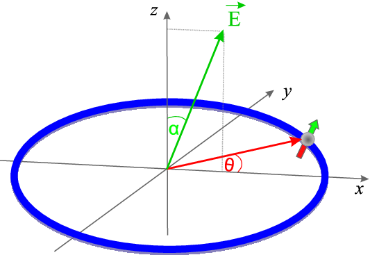
We now focus on the limit of a ring potential with tight harmonic confinement in the transverse direction. Then, for sufficiently weak interaction strength, the transverse motion is frozen in the lowest-energy mode, which is a Gaussian $\varphi_{{}_{0}}(\rho)=e^{-\rho^{2}/2a_{\perp}^{2}}/\sqrt{\pi}a_{\perp}$ of spatial extent $a_{\perp}\equiv$$\sqrt{\hbar/m\omega_{\perp}}\ll R$ [14]. Averaging out the transverse degrees of freedom over the reduced density matrix $\hat{\rho}_{\perp}=|\varphi_{0}\rangle\langle\varphi_{{}_{0}}|$ , one arrives at an effective 1D Hamiltonian [16]

where the angle $\theta_{i}$ specifies the position of particle $i$ on the ring. For $R\gg a_{\perp}$, the effective interaction takes the form $V_{{\rm 1D}}(\theta_{1},\theta_{2})=V_{{\rm CM}}\left(\Theta\right)V_{{\rm rel}}(\vartheta)$, where $\Theta=(\theta_{1}+\theta_{2})/2$ is the center-of-mass (CM) angle of the two dipoles and $\vartheta=\theta_{1}-\theta_{2}$ is the relative angle. In terms of $s=2R|\sin(\vartheta/2)|/a_{\perp}$, the dependence on the relative angle is given by

moreover,

Note that the effective interaction $V_{\mathrm{1D}}$ is inhomogeneous in the angular coordinates: This reflects the anisotropy of the underlying 3D interaction, which favors configurations where the two dipoles are arranged preferably parallel to $\mathbf{d}$, i.e., such that $\cos\theta_{rd}=\sin\alpha\sin\left({\scriptstyle\frac{\theta_{1}+\theta_{2}}{2}}\right)$ is maximized, with the particles restricted to the ring. Thus the CM potential, shown in Fig. 2, has minima at $\Theta=\pm\frac{\pi}{2}$, which become more pronounced for larger $\alpha$. For

the potential acquires attractive regions. The potential should be viewed as a potential-energy surface which depends on both particles’ coordinates rather than just the distance between them, as sketched in Fig. 2.

The derivation of the effective interaction (2) assumes that the single-mode approximation is valid, i.e., that only the lowest transverse mode $\varphi_{0}$ is occupied. This is equivalent to first-order perturbation theory or, in the language of scattering theory, the Born approximation (where $\varphi_{0}(\rho)e^{iqx}$ replaces the 3D plane-wave states in the presence of confinement). This is valid so long as the interaction energy is small compared with the transverse level spacing, $\hbar\omega_{\perp}$, i.e., if $r_{d}\ll a_{\perp}$. In that case, second-order perturbation theory predicts negative corrections $O(\frac{r_{d}}{a_{\perp}})^{2}$ due to virtual excitation of higher transverse levels. For interaction energies of order $\hbar\omega_{\perp}$, confinement-induced resonances may be expected, similar to those for contact interactions under transverse confinement [28, 14].

Let us briefly discuss some properties of the two-body relative problem, given by the Hamiltonian

Strictly speaking, this is relevant only if CM and relative motions decouple – as in the case of dipoles perpendicular to the plane of the ring ($\alpha=0$), but also, more generally, for a linear geometry [14]. However, it will also provide useful insight in cases where the particle spacing is small compared with the length scale on which $V_{CM}$ varies, so that one may locally replace $D^{2}/4a_{\perp}^{3}\equiv V_{\mathrm{CM}}(\Theta)$ at fixed $\Theta$.

For distances $|r|\gg a_{\perp}$, the free-space dipolar potential is restored, so that the Hamiltonian becomes $a_{\perp}$ independent,

Its strength is characterized by the dipolar length

At short distances, the transverse average introduces a short-range “cutoff” $a_{\perp}$. This attenuates the $r=0$ divergence into a peak of order $D^{2}/a_{\perp}^{3}$.¹¹ 1 A straightforward way of seeing this is by replacing the transverse Gaussian by a plane wave, $\varphi_{0}(\rho)=\frac{1}{\sqrt{2\pi a_{\perp}}}$, $\rho<a_{\perp}/2$: Then the 1D interaction would have the form $D^{2}/\sqrt{a_{\perp}^{2}+\rho^{2}}^{3}$.

As an illustration, we have diagonalized $h_{\mathrm{rel}}$ numerically and plotted the ground-state wave function $\psi_{\mathrm{rel}}(\vartheta)$ in Fig. 3 for different $r_{d}/R$. For bosons, the noninteracting wave function is the zero-momentum state $\psi(\vartheta)=\frac{1}{\sqrt{2\pi}}$. For $r_{d}/R\ll 1$, the dominant contribution comes from the peak of $V_{\mathrm{rel}}$ at $\vartheta=0$, where the probability amplitude is reduced. With increasing $r_{d}$, the minimum value of $\psi(0)$ becomes deeper until it reaches down to almost zero (see, e.g., $r_{d}/R=0.4$), in which case $\psi(\vartheta)\sim|\sin\frac{\vartheta}{2}|$ resembles the modulus of the wave function of noninteracting fermions. This behavior is reminiscent of bosons with a short-range (contact) interaction.

For $r_{d}/R\gtrsim 1$, the weaker $|r|^{-3}$ tail becomes effective, driving the two dipoles apart until their density is sharply peaked at a distance $|\vartheta|=\pi$ (i.e, the dipoles are at opposite poles of the ring, $|r|=2R$). This is a precursor of a crystal-like state. For fermions, the modulus $|\psi(\vartheta)|$ would look similar.

In the spirit of our comment above, let us consider an effective attraction, $r_{d}<0$. Figure 3 illustrates that two bosons form a bound state, which here becomes localized for $|r_{d}|/R\gtrsim 0.01$. This is analogous to the well-known bound state of a 1D delta interaction. However, even identical fermions can form a “p-wave” bound state (Fig. 3, inset), provided the potential is deep enough to accommodate a second, anti-symmetric level. Note that it owes its existence to the non-zero range $\sim a_{\perp}$ of the potential.

Let us mention that the relative state for $N=2$ fermions (or any even number) on a ring is a subtle issue, as can be seen from the Slater determinant $(e^{\pm i\theta_{2}}-e^{\pm i\theta_{1}})\propto e^{\pm i\frac{\theta_{1}+\theta_{2}}{2}}\sin\frac{\theta_{1}-\theta_{2}}{2}$. The CM state has nonzero (angular) momentum $\pm 1$, whereas the relative orbital, having momentum $\frac{1}{2}$, is antiperiodic in $\vartheta\equiv\theta_{1}-\theta_{2}$ in order to preserve $2\pi$-periodicity of the total wave function. This relates to the fact that any even-$N$ Fermi sea is twofold degenerate, and thus will either have nonzero momentum or, in the case of a symmetric Fermi-level state $e^{ik_{F}\theta_{N}}+e^{-ik_{F}\theta_{N}}\propto\cos(k_{F}\theta_{N})$, a cosine modulation of the CM wave function, breaking the translational symmetry.

Since the number density $n(\theta)=\langle\sum_{i}\delta(\theta-\theta_{i})\rangle=N/2\pi$ is constant for any $nr_{d}$ due to translational invariance in $\theta$, we focus on two-particle correlations. These are described, e.g., by the pair distribution function $\rho_{2}(\theta,\theta^{\prime})=\sum_{i\neq j}\langle\delta(\theta-\theta_{i})\delta(\theta^{\prime}-\theta_{j})\rangle$, which gives the probability density of finding one dipole at $\theta$ and a second one at $\theta^{\prime}$. This is plotted in Fig. 4 for $N=4$ bosons.

For dipole lengths much smaller than the inter-particle distance, $nr_{d}\ll 1$, the initially uniform pair distribution develops a “correlation hole” at $\theta=\theta^{\prime}$ with increasing coupling — indicating that finding two dipoles at the same position becomes more and more unlikely — until the pair distribution strongly resembles that of noninteracting fermions (see, e.g., $nr_{d}=0.25$) exhibiting Friedel oscillations. This gas-like behavior is reminiscent of bosons interacting through a short-range or contact interaction $g\delta(x-x^{\prime})$ [29], an observation similarly made in the context of a dipolar gas in a harmonic trap [30]. Throughout this regime, fermions would remain essentially noninteracting due to the Pauli principle.

As the dipolar length becomes comparable with the mean inter-particle separation, $nr_{d}\gtrsim 1$, the long-range tail of the interaction becomes crucial. Then the pair distribution develops more pronounced oscillations, which culminate in well-separated peaks for $nr_{d}\gg 1$. These indicate the crystal-like localization of the individual particles [10, 30].

For weak dipolar coupling, $r_{d}\ll 1/n$, we observe a behavior reminiscent of a 1D Bose gas with short-range interactions. Let us now model this gas-like regime.

The 1D Bose gas is described by the Lieb-Liniger model [29]

where here $x_{i}\equiv R\theta_{i}$. In the thermodynamic limit $N,R\to\infty$ (keeping the density $n=N/2\pi R$ fixed), the properties of the Lieb-Liniger model are completely determined by the dimensionless parameter [29]

where $a_{1}=-2\hbar^{2}/mg$ denotes the 1D scattering length. More specifically, the Lieb-Liniger gas exhibits a crossover from a weakly interacting Bose gas for $\gamma\ll 1$ to a so-called Tonks gas in the “fermionization” limit $\gamma\gg 1$, similar to our findings in the gas-like regime. We will now delineate a relation between the model parameter $\gamma$ (i.e., $g$) and the 1D dipolar interaction (parametrized by $r_{d},a_{\perp}$).

Let us now discuss the limiting case $nr_{\mathrm{d}}\gg 1$. We found that the long-range dipolar repulsion becomes dominant here, so that the particles localize. Another indicator of this is the ground-state energy of the dipoles (Fig. 5), which deviates from the saturated fermionization regime and changes over to an energy increase proportional to $r_{\mathrm{d}}$ for $nr_{d}\gg 1$. In this regime, the dipoles become classical in the sense that the potential energy overwhelms the kinetic energy, so that for $nr_{d}\to\infty$ the ground state becomes a position eigenstate $|\bar{\theta}_{1},\dots,\bar{\theta}_{N}\rangle_{\pm}$ ($\pm$ indicating bosonic/fermionic permutation symmetry), where the angles $\{\bar{\theta}_{j}\}$ are determined by minimizing the energy

This yields a crystal-like, equidistant distribution of particles: $\bar{\theta}_{j}=j\frac{2\pi}{N}+\delta$, $j\in\{0,\dots,N-1\}$, which is only defined up to an angle $\delta$ by rotational invariance, and an energy $E_{C}=\frac{ND^{2}}{16R^{3}}\sum_{\nu=1}^{N-1}\left|\sin\frac{\nu\pi}{N}\right|^{-3}$. To find the behavior in the thermodynamic limit, one may approximate the sum by an integral, $\sum_{\nu}\left|\sin\frac{\nu\pi}{N}\right|^{-3}\approx 2\frac{N}{\pi}\int_{\pi/2N}^{\pi/2}d\phi\left|\sin\phi\right|^{-3}\simeq 4N^{3}/\pi^{3}$ as $N\to\infty$. In that limit, we thus have $E_{C}/N\approx 2nr_{d}\times(\hbar n)^{2}/2m$, an expression formally similar to that of an infinite line [10].

However, for finite $nr_{d}$, the particles are not strictly localized. Rather, their wave packets are spread out over a width $w$ due to their zero-point motion, as is illustrated by the pair distribution function in Fig. 4. We now estimate $w$. For simplicity, we consider a linear 1D system and perform a classical normal-mode analysis: Expanding the interaction potential $D^{2}\sum_{i<j}|x_{i}-x_{j}|^{-3}$ to second order about the minimum (a lattice with nearest-neighbor distance $1/n$) yields effective harmonic-oscillator frequencies $\omega_{C}=\sqrt{12D^{2}n^{5}/m}$, corresponding to an oscillator width $w\equiv\sqrt{\hbar/m\omega_{C}}$ given by

This confirms that for dipole lengths large compared to the average inter-particle spacing, $nr_{\mathrm{d}}\gg 1$, the dipoles should indeed be well localized, in agreement with Fig. 4. Taking into account the zero-point motion about the classical equilibrium positions, we find that the crystal energy $E_{C}$ is corrected by $+N\hbar\omega_{C}/2\sim N(\hbar n)^{2}/m\times\sqrt{nr_{d}/2}$.

In the crystalline limit $nr_{d}\to\infty$ where the behavior is nearly classical, the same reasoning applies to fermions. For finite coupling, however, due to the Pauli principle, the kinetic energy of fermions is inherently higher than that of bosons. In this sense, stronger repulsion is needed to suppress the zero-point motion compared to bosons, so that the crystalline limit is approached more slowly.

To bring out the essential effect, we first focus on bosons with an inhomogeneity just below the threshold value, $\alpha=0.19\pi\lesssim\alpha_{\mathrm{c}}$. In contrast to dipoles aligned perpendicular to the plane of the ring, for $\alpha\neq 0$ the system is no longer rotationally invariant about $\theta$. Thus interaction effects are reflected in the number density $n(\theta)$, as shown for $N=4$ bosons in Fig. 7. For small couplings, $nr_{d}\ll 1$, the state resembles that of a Bose gas. The density has a slightly stronger weight near the potential minima $\theta=\pm\pi/2$ for intermediate couplings but tends to flatten out for larger values, $nr_{d}\sim 1$. By contrast, for $nr_{d}\gg 1$, the density profile develops $N=4$ distinct peaks, revealing a crystal-like localization of the particles. Note that the peak positions are not equidistant, but rather slightly displaced toward $\theta=\pm\pi/2$ due to the pronounced minima of $V_{\mathrm{CM}}$.²² 2 For an odd number of dipoles, localization is more subtle. For, say, $N=3$, there are two degenerate ground states classically – one would thus see a symmetry-averaged $2N=6$ peaks in the density $n(\theta)$, rather just $N=3$.

The transition from a gas-like to a localized state is also clearly visible in the pair distribution function $\rho_{2}(\theta,\theta^{\prime})$ shown in Fig. 7: For $nr_{d}\ll 1$, two-body correlations are absent in the mean-field regime, $\rho_{2}(\theta_{1},\theta_{2})\approx\rho(\theta_{1})\rho(\theta_{2})$, or are limited to Friedel-like oscillations around the correlation hole near $\theta_{1}=\theta_{2}$, reminiscent of a fermionized Bose gas. For $nr_{d}\gg 1$, the pinning of the particles to individual peaks is clearly discernible.

A similar trend would be observed for fermions: For $nr_{d}\ll 1$, we find a gas-like state, which however is only weakly interacting owing to the Pauli exclusion principle. With increasing coupling, $nr_{d}\gtrsim 1$, the state crosses over into a crystal-like one characterized by localization of the particles in the classical minimum-energy configuration, just as in the Bose case. Due to the Fermi energy, that crossover is much smoother than for the bosons.

Let us dwell on the parameter range where the ground state is gas-like. In the homogeneous limit $\alpha\to 0$, we established that here the system is well described by the Lieb-Liniger Hamiltonian (3), with the 1D interaction strength $g=D^{2}/a_{\perp}^{2}$ (for $r_{d}\ll a_{\perp}$). By extension, for $\alpha\neq 0$, the system should resemble a Bose gas with an inhomogeneous interaction $g\left(\frac{x_{1}+x_{2}}{2}\right)\delta(x_{1}-x_{2})$, where $g(x)=D^{2}(1-3\sin^{2}\alpha\sin^{2}\frac{x}{R})/a_{\perp}^{2}$ is the Fourier transform of $V_{1D}$ at zero relative momentum.

Although this inhomogeneous Lieb-Liniger Hamiltonian system is not integrable, some insight can be gained by assuming slow variation of $g(x)$ compared with the local correlation length. In this case, a local-density approximation [36] may be applied, which consists in assuming the equation of state of the homogeneous Lieb-Liniger system, $\mu=f_{g}(n)$, to hold locally, $\mu=f_{g(x)}[n(x)]$. Here $\mu$ denotes the chemical potential as a function of number density $n(x)$; moreover, for the Lieb-Liniger system, $f_{g}(n)$ can be obtained directly from the ground-state energy, which is known in terms of the dimensionless function $e(\gamma)=E/N\frac{(\hbar n)^{2}}{2m}$ [29, 37]. Note that the chemical potential is $x$ independent, as local equilibrium is assumed to hold. Carrying out the local-density approximation numerically for the full range of $\gamma$ is beyond the present scope. However, considering the borderline case also provides some insight into the impact of the inhomogeneity.

We now present analytical models for the crystal-like limit $nr_{d}\gg 1$. Similarly to the case $\alpha=0$ , here each dipole is pinned to a position $\bar{\theta}_{i}$ determined by the extrema of the classical energy

In this case, though, the equilibrium configuration is not simply an equidistant lattice. Rather, owing to the competition of potential energy of the relative motion (favoring maximum distance) and the CM (alignment near $\theta=\pm\pi/2$), the dipoles are localized at discrete positions which are distributed inhomogeneously on the ring. In principle, the distribution of $\{\bar{\theta}_{i}\}$ can be found by numerical minimization of $E_{C}$. However, to obtain some analytic insight, we will do this for one of the simplest nontrivial cases, $N=4$. Complementing this few-body viewpoint, we then extend the local-density approximation above to the strong-coupling regime.

Let us first illustrate the crossover from weak to strong coupling by means of the density $n(\theta)$, shown in Fig. 8 ($N=4$ bosons, $\alpha=0.2\pi$) and Fig. 9 ($N=3$ fermions, $\alpha=0.22\pi$). In both cases, the densities go over from a homogeneous profile, characteristic of a gas-like state, to one with two sharp peaks, indicating cluster formation.

It is noteworthy that in these examples, the transition to the localized clustered state is very sharp (e.g., at $nr_{d}\approx 0.8$ for the bosons). This is also reflected in the ground-state energy $E(nr_{d})$, shown in Fig. 10. In fact, whereas the energy eventually falls and becomes negative at high enough $nr_{d}$ for any $\alpha>\alpha_{c}$, the behavior for small coupling crucially depends on $\alpha$: Closer to the critical angle, the bosonic energy increases for small coupling, and it is only beyond a critical value of $nr_{d}$ that it starts decreasing rather abruptly. By contrast, for larger $\alpha$, $E(nr_{d})$ is a monotonically decreasing function. To understand that competition between repulsion and attraction, note that—for $nr_{d}\to 0$—the (bosonic) energy behaves as

where the average is over the (uniform) noninteracting CM and relative states. Since $g(0)>0$, the energy increase for small $nr_{d}$ is positive for

In other words, for tilt angles less than $\alpha_{c}$, the potential is predominantly repulsive. Initially, the delocalized bosons will thus undergo an analogous evolution as in Sec. IV, e.g., behave like an inhomogeneous Bose gas, which is predominantly repulsive ($\alpha<\alpha_{c2}$) or has a net attraction ($\alpha>\alpha_{c2}$). For identical fermions, the interaction-energy shift per particle will be negligible compared with the Fermi energy for all $\alpha$.

This makes clear that the transition to a clustered state also strongly depends on $\alpha$. Beyond $\alpha_{c2}$, there is a smooth crossover from an attractive gaseous state to a clustered one (Fig. 10) at rather small coupling. By contrast, for only slightly overcrtical $\alpha\in(\alpha_{c},\alpha_{c2})$ – e.g., $\alpha=0.2\pi$ in Fig. 8 – the transition takes place at much larger coupling and is more subtle. With increasing $nr_{d}$, the repulsive gas-like state first goes over into a transitional state with strong fragmentation (cf. $nr_{d}=0.802$), which can be thought of roughly as a Mott-insulator-type state $|\frac{N}{2},\frac{N}{2}\rangle$ with $N/2$ dipoles at each of the poles, $\theta=\pm\pi/2$. This can be best seen from the pair distribution $\rho_{2}(\theta,\theta^{\prime})$, Fig. 8(center), which upon closer inspection confirms that a measurement of one particle at, say, $\pi/2$ yields a measurement of $(\frac{N}{2}-1)$ particles at $\pi/2$ and $\frac{N}{2}$ at $-\pi/2$. There is a sharp avoided crossing to a clustered state ($nr_{d}=0.807$), with all $N$ particles localized at either $\pm\pi/2$. By parity symmetry, the exact ground state is actually a superposition or Schrödinger-cat state, $\frac{1}{\sqrt{2}}\left(|N,0\rangle+|0,N\rangle\right)$, as is evident from the pair distribution function in Fig. 8. A small symmetry-breaking perturbation will likely cause a collapse of the superposition.

For fermions, the critical interaction strength needed for cluster formation is higher (Fig. 10). This is because of the Pauli principle: The exchange hole discernible in $\rho_{2}$ (Fig. 9) strongly reduces the average attraction between two fermions. Moreover, due to the Pauli pressure, the fermions are more spread out spatially and require a stronger attraction to be squeezed into the narrow zone of attraction.

To obtain a deeper understanding of cluster formation, including its dependence on the particle number and on $\alpha$, we will now develop a simplified analytical model that can reproduce its basic features.

As a first step, let us consider the case of a homogeneous system with purely attractive interaction. This is interesting in its own right, since clustered states are not limited to a ring geometry. Moreover, as we will see below, this also allows for a qualitative understanding of the inhomogeneous case.

References

- [1] M. A. Baranov, Phys. Rep. 464, 71 (2008).
- [2] T. Lahaye, C. Menotti, L. Santos, M. Lewenstein, and T. Pfau, Rep. Prog. Phys. 72, 126401 (2009).
- [3] T. Lahaye, T. Koch, B. Froehlich, M. Fattori, J. Metz, A. Griesmaier, S. Giovanazzi, and T. Pfau, Nature 448, 672 (2007).
- [4] M. Lu, S. H. Youn, and B. L. Lev, Phys. Rev. Lett. 104, 063001 (2010).
- [5] S. Ospelkaus, K. Ni, G. Quéméner, B. Neyenhuis, D. Wang, M. de Miranda, J. Bohn, J. Ye, and D. Jin, Phys. Rev. Lett. 104, 30402 (2010).
- [6] J. Deiglmayr, A. Grochola, M. Repp, K. Mörtlbauer, C. Glück, J. Lange, O. Dulieu, R. Wester, and M. Weidemüller, Phys. Rev. Lett. 101, 133004 (2008).
- [7] J. M. Sage, S. Sainis, T. Bergeman, and D. DeMille, Phys. Rev. Lett. 94, 203001 (2005).
- [8] T. Koch, T. Lahaye, J. Metz, B. Fröhlich, A. Griesmaier, and T. Pfau, Nature Phys. 4, 218 (2008).
- [9] K. Ni, S. Ospelkaus, D. Wang, G. Quéméner, B. Neyenhuis, M. de Miranda, J. Bohn, J. Ye, and D. Jin, Nature 464, 1324 (2010).
- [10] A. S. Arkhipov, G. E. Astrakharchik, A. V. Belikov, and Y. E. Lozovik, JETP Lett. 82, 39 (2005).
- [11] R. Citro, E. Orignac, S. De Palo, and M. Chiofalo, Phys. Rev. A 75, 51602(R) (2007).
- [12] S. De Palo, E. Orignac, R. Citro, and M. Chiofalo, Phys. Rev. B 77, 212101 (2008).
- [13] P. Pedri, S. De Palo, E. Orignac, R. Citro, and M. Chiofalo, Phys. Rev. A 77, 15601 (2008).
- [14] S. Sinha and L. Santos, Phys. Rev. Lett. 99, 140406 (2007).
- [15] G. Astrakharchik, G. Morigi, G. De Chiara, and J. Boronat, Phys. Rev. A 78, 63622 (2008).
- [16] O. Dutta, M. Jääskeläinen, and P. Meystre, Phys. Rev. A 73, 043610 (2006).
- [17] K. T. Law and D. E. Feldman, Phys. Rev. Lett. 101, 096401 (2008).
- [18] M. Abad, M. Guilleumas, R. Mayol, M. Pi, and D. M. Jezek, Phys. Rev. A 81, 043619 (2010).
- [19] M. Abad, M. Guilleumas, R. Mayol, M. Pi, and D. M. Jezek, Europhys. Lett. 94, 10004 (2011).
- [20] M. Maik, P. Buonsante, A. Vezzani, and J. Zakrzewski, arXiv:1107.1103 (2011).
- [21] A. Ramanathan, K. C. Wright, S. R. Muniz, M. Zelan, W. T. Hill, C. J. Lobb, K. Helmerson, W. D. Phillips, and G. K. Campbell, Phys. Rev. Lett. 106, 130401 (2011).
- [22] L. Amico, A. Osterloh, and F. Cataliotti, Phys. Rev. Lett. 95, 063201 (2005).
- [23] S. Gupta, K. W. Murch, K. L. Moore, T. P. Purdy, and D. M. Stamper-Kurn, Phys. Rev. Lett. 95, 143201 (2005).
- [24] A. S. Arnold, C. S. Garvie, and E. Riis, Phys. Rev. A 73, 041606 (2006).
- [25] W. H. Heathcote, E. Nugent, B. T. Sheard, and C. J. Foot, New J. Phys. 10, 043012 (2008).
- [26] K. Henderson, C. Ryu, C. MacCormick, and M. G. Boshier, New J. Phys. 11, 043030 (2009).
- [27] S. Zöllner, G. M. Bruun, C. J. Pethick, and S. M. Reimann, Phys. Rev. Lett. 107, 035301 (2011).
- [28] M. Olshanii, Phys. Rev. Lett. 81, 938 (1998).
- [29] E. H. Lieb and W. Liniger, Phys. Rev. 130, 1605 (1963).
- [30] F. Deuretzbacher, J. C. Cremon, and S. M. Reimann, Phys. Rev. A 81, 063616 (2010).
- [31] K. Sakmann, A. I. Streltsov, O. E. Alon, and L. S. Cederbaum, Phys. Rev. A 72, 033613 (2005).
- [32] M. Girardeau, J. Math. Phys. 1, 516 (1960).
- [33] G. E. Astrakharchik, J. Boronat, J. Casulleras, and S. Giorgini, Phys. Rev. Lett. 95, 190407 (2005).
- [34] G. E. Astrakharchik and Y. E. Lozovik, Phys. Rev. A 77, 013404 (2008).
- [35] T. Nagamiya, Proc. Phys.-Math. Soc. Jpn 22, 705 (1940).
- [36] J. Oliva, Phys. Rev. B 38, 8811 (1988).
- [37] V. Dunjko, V. Lorent, and M. Olshanii, Phys. Rev. Lett. 86, 5413 (2001).
- [38] C. J. Pethick and H. Smith, Bose-Einstein condensation in dilute gases, 2nd ed. (Cambridge University Press, Cambridge, 2008).
- [39] D. M. Gangardt and G. V. Shlyapnikov, Phys. Rev. Lett. 90, 010401 (2003).
- [40] J. B. McGuire, J. Math. Phys. 5, 622 (1964).
- [41] Y. Castin and C. Herzog, C. R. Acad. Sci., Ser IV 2, 419 (2001).
- [42] G. J. Milburn, J. Corney, E. M. Wright, and D. F. Walls, Phys. Rev. A 55, 4318 (1997).
- [43] E. J. Mueller, T.-L. Ho, M. Ueda, and G. Baym, Phys. Rev. A 74, 033612 (2006).
- [44] B. Wunsch, N. T. Zinner, I. B. Mekhov, S.-J. Huang, D.-W. Wang, and E. Demler, Phys. Rev. Lett. 107, 073201 (2011).
- [45] M. Dalmonte, P. Zoller, and G. Pupillo, Phys. Rev. Lett. 107, 163202 (2011).
- [46] M. H. Beck, A. Jäckle, G. A. Worth, and H.-D. Meyer, Phys. Rep. 324, 1 (2000).
- [47] S. Zöllner, H.-D. Meyer, and P. Schmelcher, Phys. Rev. A 74, 053612 (2006).
- [48] H.-D. Meyer and G. A. Worth, Theor. Chem. Acc. 109, 251 (2003).