The Aharonov-Bohm effect in scattering of short-wavelength particles

The theoretical prediction of the Aharonov-Bohm (AB) effect in 1959 [1] was one of the most intriguing achievements in quantum theory. Now this effect has been long recognized for its crucial role in demonstrating that, in addition to the usual local (classical) influence of electromagnetic field on charged particles, there exists the unusual nonlocal (purely quantum) influence of electromagnetic fluxes confined in the regions which are inaccessible to charged particles (see, e.g., reviews [2, 3]). A particular example is quantum-mechanical scattering of nonrelativistic charged particles by an impenetrable straight and infinitely long solenoid that encloses a magnetic flux: as was shown in [1], this process depends periodically on the value of the enclosed flux. Although a formula for the differential cross section of this process was derived in Section 4. ”Exact solution for scattering problems” of [1], the formula was never checked experimentally. Perhaps, it was not even intended to be checked, since the authors [1] in the preceding sections of their work proposed a closely related, but different from the scattering one, experiment to confirm their theoretical prediction; this experiment consisted in observing a fringe shift in the interference pattern due to two coherent particle beams under the influence of an impenetrable magnetic vortex placed between the beams. Since then the theory and the experiment for the AB effect followed their own non-intersecting ways. The concern of experimentalists was to exclude completely penetration of the particle beams into the region of nonzero magnetic flux, see [3]. As to the theoretical development, scattering theory initiated by Aharonov and Bohm was substantiated and further elaborated, see [4, 5, 6].

It should be noted that the concern of theoreticians was mostly in the case of long-wavelength scattered particles, when the transverse size of the magnetic vortex was neglected. Since a direct scattering experiment is hard to perform with long-wavelength (slowly moving) particles, thus elaborated theory remained actually unverified. On the one hand, as the particle wavelength decreases, the perspectives of performing a scattering experiment with such particles are increasing. On the other hand, the transverse size of the vortex then comes into play, and, given the technical difficulties of measuring the interference AB effect, it may seem hardly possible to avoid the particle penetration inside the vortex in a direct scattering experiment. However, as we shall see, these misgivings are irrelevant for the case of short-wavelength (fast-moving) particles. The aim of the present paper is to extend scattering theory to such a case (see also [7, 8, 9]) and to reach the realm where the experimental verification of the scattering AB effect is quite feasible.

First, let us recall briefly the setup which is conventionally used for the experimental verification of the AB effect (see, e.g., [2, 3]). It involves the observation of the interference patterns resulting from the two coherent electron beams bypassing from different sides an impenetrable magnetic vortex which is orthogonal to the plane defined by the beams. This is a so called double-slit interference experiment, although in reality an electrostatic biprism is used to bend the beams and to direct them on the detection screen. Let the detection screen be parallel to the screen with slits, $L$ be the distance between the screens, and $D$ be the distance between the slits. Otherwise, in the biprism setting, the line connecting images of a source is parallel to the detection screen, $L^{\prime}$ is the distance between the line and the screen, and $D^{\prime}$ is the distance between the images; since the interference pattern depends on quotient $D^{\prime}/L^{\prime}$ rather than on $L^{\prime}$ and $D^{\prime}$ separately, the primes will be dropped in the following. The interference pattern on the detection screen consists of equally spaced fringes which are in the same direction as the magnetic vortex,

$$I(y)=4I_{0}(y)\cos^{2}\left[\left(\frac{yD}{\lambda L}+\frac{\Phi}{\Phi_{0}}\right)\pi\right],$$

(1)

where $y$ is the coordinate which is orthogonal to the fringes on the detection screen ($y=0$ corresponds to the point which is symmetric with respect to the slits), $I_{0}(y)$ is the intensity in the case when either of the slits is closed, $\lambda$ is the electron wavelength, $\Phi$ is the flux of the impenetrable magnetic vortex placed just after the screen with slits (otherwise, after the biprism), $\Phi_{0}=hce^{-1}$ is the London flux quantum. Intensity $I(y)$ (1) is oscillating with period

$$\Delta=\lambda LD^{-1},$$

(2)

and the enveloping function is given by $4I_{0}(y)$ which is a Gaussian centred at $y=0$. At the centre of the detection screen one gets

$$I(0)=4I_{0}(0)\cos^{2}\left(\frac{\Phi}{\Phi_{0}}\pi\right).$$

(3)

If $L\gg D$ and $\lambda$, then one can use dimensionless (angular) variable $\varphi=y/L$. The period of oscillations in this variable is

$$\delta=\lambda D^{-1}.$$

(4)

Evidently, the period of oscillation decreases with the decrease of wavelength $\lambda$. The linear resolution of the detector should be at least as high as $\frac{1}{2}\Delta$, that is why the observation of the interference pattern becomes more complicated in the short-wavelength limit. Since the enveloping function takes a form of a narrow peak in this limit, it is crucial that the oscillations be distinguishable in the enveloping background. To measure this, one defines the visibility of the central point as

$$V=\frac{\left|I(0)-I\left(\pm\frac{1}{2}\Delta\right)\right|}{I(0)+I\left(\pm\frac{1}{2}\Delta\right)}.$$

(5)

In view of the symmetry of the enveloping function $\left(I_{0}\left(-\frac{1}{2}\Delta\right)=I_{0}\left(\frac{1}{2}\Delta\right)\right)$, one finds immediately

$$V=\frac{\left|I_{0}(0)\!-\!I_{0}\left(\!\frac{1}{2}\Delta\!\right)\!+\!\left[I_{0}(0)\!+\!I_{0}\left(\!\frac{1}{2}\Delta\!\right)\right]\!\cos\!\left(\!2\frac{\Phi}{\Phi_{0}}\pi\!\right)\right|}{I_{0}(0)\!+\!I_{0}\left(\frac{1}{2}\Delta\right)\!+\!\left[I_{0}(0)\!-\!I_{0}\left(\frac{1}{2}\Delta\right)\right]\!\cos\!\left(2\frac{\Phi}{\Phi_{0}}\pi\right)}.$$

(6)

It should be noted that visibility (5) is nonzero in the case of the absence of oscillations: $V=|I_{0}(0)-I_{0}(\Delta/2)|/[I_{0}(0)+I_{0}(\Delta/2)]$. This case is mimicked at $\Phi=(n\pm 1/4)\Phi_{0}$ and $\Phi=\left\{n\pm\pi^{-1}\arcsin\left[I_{0}(0)/\sqrt{I_{0}^{2}(0)+I_{0}^{2}(\Delta/2)}\right]\right\}\Phi_{0}$ ($n$ is an integer number).

Concluding this section, we note that the value of the bending potential and the distance to the detection screen should be adjusted in order that the interference pattern be visible. Such a type of adjustment is unnecessary for the diffraction pattern in direct scattering of short-wavelength particles on a magnetic vortex.

We start with the Schrödinger equation for the wave function describing the stationary scattering state,

$$H\psi(r,\,\varphi)=\frac{\hbar^{2}k^{2}}{2m}\psi(r,\,\varphi),$$

(7)

where $m$ is the particle mass and $k$ is the absolute value of the particle wave vector ($k=2\pi/\lambda$); the impenetrable magnetic vortex is assumed to be directed orthogonally to the plane with polar coordinates $r$ and $\varphi$, and we confine ourselves to the particle motion in this plane, since the motion along the vortex is free. Out of the vortex core the Schrödinger hamiltonian takes the form

$$H=-\frac{\hbar^{2}}{2m}\left[r^{-1}\partial_{r}r\partial_{r}+r^{-2}\left(\partial_{\varphi}-{\rm i}\Phi\Phi_{0}^{-1}\right)^{2}\right],$$

(8)

and we impose condition

$$\lim\limits_{r\rightarrow\infty}{\rm e}^{{\rm i}kr}\psi(r,\,\pm\pi)=1,$$

(9)

signifying that the incident wave comes from the far left; the forward direction is $\varphi=0$, and the backward direction is $\varphi=\pm\pi$.

Without a loss of generality we assume that the vortex has a shape of cylinder of radius $r_{c}$ and impose the Robin boundary condition on the wave function:

$$\left.\left\{\left[\cos(\rho\pi)+r_{c}\sin(\rho\pi)\partial_{r}\right]\psi(r,\,\varphi)\right\}\right|_{r=r_{c}}=0;$$

(10)

$\rho=0$ corresponds to the Dirichlet boundary condition (perfect conductivity of the boundary), and $\rho=1/2$ corresponds to the Neumann one (absolute rigidity of the boundary). The solution to (7) with hamiltonian (8), which satisfies conditions (9) and (10), takes the following form

$$\psi(r,\,\varphi)=\sum\limits_{n\in\mathbb{Z}}{\rm e}^{{\rm i}n\varphi}e^{{\rm i}(|n|-\frac{1}{2}|n-\mu|\pi)}\left[J_{|n-\mu|}(kr)-\Upsilon_{|n-\mu|}^{(\rho)}(kr_{c})H_{|n-\mu|}^{(1)}(kr)\right],$$

(11)

where $\mathbb{Z}$ is the set of integer numbers, $\mu=\Phi\Phi_{0}^{-1}$, $J_{\alpha}(u)$ and $H_{\alpha}^{(1)}(u)$ are the Bessel and the first-kind Hankel functions of order $\alpha$, and

$$\Upsilon_{\alpha}^{(\rho)}(u)=\frac{J_{\alpha}(u)}{H_{\alpha}^{(1)}(u)}\,\frac{\cot(\rho\pi)+u\partial_{u}\ln J_{\alpha}(u)}{\cot(\rho\pi)+u\partial_{u}\ln H_{\alpha}^{(1)}(u)}.$$

(12)

Thus, wave function (11) consists of two parts: the one which will be denoted by $\psi_{0}(r,\,\varphi)$ is independent of $r_{c}$, and the other one which will be denoted by $\psi_{c}(r,\,\varphi)$ is dependent on $r_{c}$.

Taking the asymptotics of the first part at large distances from the vortex, $kr\gg 1$, one can get (see [10])

	$\displaystyle\psi_{0}(r,\,\varphi)={\rm e}^{{\rm i}kr\cos\varphi+{\rm i}\mu\varphi}\Bigl\{\cos(\mu\pi)-{\rm i}{\rm sgn}(\varphi)\sin(\mu\pi)\Bigr.$
	$\displaystyle\Bigl.\times\left[1-{\rm e}^{{\rm i}\left(\frac{1}{2}+[\![\mu]\!]-\mu\right)\varphi}{\rm erfc}\left({\rm e}^{-{\rm i\pi/4}}\sqrt{2kr}\left|\sin\frac{\varphi}{2}\right|\right)\right]\Bigr\},$		(13)

where $[\![u]\!]$ denotes the integer part of quantity $u$ (i.e. the integer which is less than or equal to $u$), ${\rm sgn}(u)=\left\{\begin{array}[]{cc}1,&u>0\\ -1,&u<0\end{array}\right\}$, ${\rm erfc}(z)=\frac{2}{\sqrt{\pi}}\int\limits_{z}^{\infty}du\,{\rm e}^{-u^{2}}$ is the complementary error function, and it is implied that $-\pi<\varphi<\pi$. In the case $\sqrt{kr}\left|\sin\frac{\varphi}{2}\right|\gg 1$, one obtains

$$\psi_{0}(r,\,\varphi)={\rm e}^{{\rm i}kr\cos\varphi}{\rm e}^{{\rm i}\mu[\varphi-{\rm sgn}(\varphi)\pi]}+f_{0}(k,\,\varphi)\frac{{\rm e}^{{\rm i}(kr+\pi/4)}}{\sqrt{r}},$$

(14)

where

$$f_{0}(k,\,\varphi)={\rm i}\frac{{\rm e}^{{\rm i}\left([\![\mu]\!]+\frac{1}{2}\right)\varphi}}{\sqrt{2\pi k}}\frac{\sin(\mu\pi)}{\sin(\varphi/2)}$$

(15)

is the scattering amplitude which was first obtained by Aharonov and Bohm [1]. In the case $kr\gg 1$ but $\sqrt{kr}\left|\sin\frac{\varphi}{2}\right|\ll 1$, one obtains

$$\psi_{0}(r,\,\varphi)={\rm e}^{{\rm i}kr\cos\varphi}\cos(\mu\pi).$$

(16)

Taking the large-distance asymptotics of the $r_{c}$-dependent part of the wave function, one gets

$$\psi_{c}(r,\,\varphi)=f_{c}(k,\,\varphi)\frac{{\rm e}^{{\rm i}(kr+\pi/4)}}{\sqrt{r}},$$

(17)

where

$$f_{c}(k,\,\varphi)={\rm i}\sqrt{\frac{2}{\pi k}}\sum\limits_{n\in\mathbb{Z}}{\rm e}^{{\rm i}n\varphi}{\rm e}^{{\rm i}(|n|-|n-\mu|\pi)}\Upsilon_{|n-\mu|}^{(\rho)}(kr_{c}).$$

(18)

In the long-wavelength limit, $kr_{c}\ll 1$, amplitude $f_{c}$ (18) is suppressed by powers of $kr_{c}$ as compared to amplitude $f_{0}$ (15); however, as was already mentioned, this limit is not feasible to experimental measurements. In the short-wavelength limit, $kr_{c}\gg 1$, amplitude $f_{0}$ (15) is suppressed and wave function $\psi_{0}$ (13) is actually reduced to a plane wave, ${\rm e}^{{\rm i}kr\cos\varphi}$, which is distorted by the flux-dependent factors, see (16) and the first term in (14). Amplitude $f_{c}$ (18) in this limit takes form [9]

	$\displaystyle f_{c}(k,\,\varphi)={\rm i}\sqrt{\frac{2\pi}{k}}\left[\cos(\mu\pi)\Delta^{([\![\mu]\!])}_{kr_{c}}(\varphi)-\sin(\mu\pi)\Gamma^{([\![\mu]\!])}_{kr_{c}}(\varphi)\right]$
	$\displaystyle-\sqrt{\frac{r_{c}}{2}|\sin(\varphi/2)|}\exp\left\{-2{\rm i}kr_{c}|\sin(\varphi/2)|+{\rm i}\mu[\varphi-{\rm sgn}(\varphi)\pi]\right\}$
	$\displaystyle\times\exp\left\{-{\rm i}\left[2\chi^{(\rho)}(kr_{c},\varphi)+\pi/4\right]\right\}+\sqrt{r_{c}}O\left[(kr_{c})^{-1/6}\right],\,\,kr_{c}\gg 1,$		(19)

where

$$\Delta_{x}^{([\![\mu]\!])}(\varphi)=\frac{1}{2\pi}\sum\limits_{|n-\mu|\leq x}{\rm e}^{in\varphi},\,\,\,\,\,\,\Gamma_{x}^{([\![\mu]\!])}(\varphi)=\frac{1}{2\pi{\rm i}}\sum\limits_{|n-\mu|\leq x}{\rm sgn}(n-\mu){\rm e}^{{\rm i}n\varphi},$$

(20)

and

$$\chi^{(\rho)}(kr_{c},\varphi)={\rm arctan}\left[\frac{2kr_{c}|\sin^{3}(\varphi/2)|}{2{\rm cot}(\rho\pi)\sin^{2}(\varphi/2)-1}\right].$$

(21)

This amplitude satisfies the optical theorem of the unusual form due to the long-range nature of the interaction with a vortex [7]:

$$2\sqrt{\frac{2\pi}{k}}\cos(\mu\pi){\rm Im}f_{c}(k,\,0)+4r_{c}\sin^{2}(\mu\pi)=\int\limits_{-\pi}^{\pi}{\rm d}\varphi|f_{c}(k,\,\varphi)|^{2}.$$

(22)

The differential cross section¹¹ 1 It is a cross section per unit length along the vortex axis, hence its dimension is that of length. in the short-wavelength limit is given by expression

	$\displaystyle\frac{{\rm d}\sigma}{{\rm d}\varphi}\equiv|f_{c}(k,\varphi)|^{2}=2r_{c}\biggl\{\cos(2\mu\pi){\Delta}_{kr_{c}}(\varphi)\biggr.$
	$\displaystyle\biggl.+\!\left[1\!-\!\cos(2\mu\pi)\!-\!\sin(2\mu\pi)\sin(kr_{c}\varphi)\right]{\Delta}_{\frac{1}{2}kr_{c}}(\varphi)\!\biggr\}\!+\!\frac{r_{c}}{2}\left|\sin\frac{\varphi}{2}\right|,$		(23)

where

$$\Delta_{x}(\varphi)=\frac{1}{4\pi x}\frac{\sin^{2}(x\varphi)}{\sin^{2}(\varphi/2)}\qquad(-\pi<\varphi<\pi)$$

(24)

is a strongly peaked at $\varphi=0$ and $x\gg 1$ function which can be regarded as a regularization of the angular delta-function,

$$\lim\limits_{x\rightarrow\infty}\Delta_{x}(\varphi)=\frac{1}{2\pi}\sum\limits_{n\in\mathbb{Z}}{\rm e}^{{\rm i}n\varphi},\,\,\,\,\,\,\Delta_{x}(0)=\frac{x}{\pi}.$$

(25)

The first term on the right-hard side of (23) describes the forward peak of the Fraunhofer diffraction on the vortex, while the last term describes the classical reflection from the vortex according to the laws of geometric (ray) optics. It should be noted that the scattering amplitude depends on the choice of a boundary condition via phase factor $\exp(-2{\rm i}\chi^{(\rho)})$, see (19) and (21); therefore, the differential cross section is independent of boundary conditions at all.

Moreover, the Fraunhofer diffraction is not affected by the penetrability of the magnetic vortex, when a boundary condition at the edge of the vortex is changed to a matching condition there. In the case of an arbitrary cylindrically symmetric configuration of the magnetic field strength inside the vortex of finite flux, the wave function in the interior of the vortex can be presented as

$$\kappa(r,\,\varphi)=\sum\limits_{n\in\mathbb{Z}}{\rm e}^{{\rm i}n\varphi}c_{n}^{(k)}\kappa_{n}(kr)\qquad(r<r_{c}),$$

(26)

where $\kappa_{n}(kr)$ is a regular solution to the appropriate partial wave equation. Matching the logarithmic derivatives of partial radial components of the solutions at the edge of the vortex, one can find that the wave function in the exterior of the vortex takes the form of (11) with $\Upsilon_{|n-\mu|}^{(\rho)}(kr_{c})$ substituted by $\Upsilon_{n}(kr_{c})$, where

$$\Upsilon_{n}(u)=\frac{J_{|n-\mu|}(u)}{H_{|n-\mu|}^{(1)}(u)}\frac{\partial_{u}\ln\kappa_{n}(u)-\partial_{u}\ln J_{|n-\mu|}(u)}{\partial_{u}\ln\kappa_{n}(u)-\partial_{u}\ln H_{|n-\mu|}^{(1)}(u)}.$$

(27)

Hence, the $r_{c}$-dependent part of the scattering amplitude is, cf. (18),

	$\displaystyle f_{c}(k,\,\varphi)={\rm i}\sqrt{\frac{2}{\pi k}}\sum\limits_{n\in\mathbb{Z}}{\rm e}^{{\rm i}n\varphi}{\rm e}^{{\rm i}(|n|-|n-\mu|)\pi}\Upsilon_{n}(kr_{c})=$
	$\displaystyle=f_{c}^{(\rm peak)}(k,\,\varphi)+f_{c}^{(\rm class)}(k,\,\varphi)+f_{c}^{(\rm res)}(k,\,\varphi),$		(28)

where

$$f_{c}^{(\rm peak)}(k,\,\varphi)=\frac{\rm i}{\sqrt{2\pi k}}\sum\limits_{|n-\mu|\leq kr_{c}}{\rm e}^{{\rm i}n\varphi}{\rm e}^{{\rm i}(|n|-|n-\mu|)\pi},$$

(29)

$$f_{c}^{(\rm class)}(k,\,\varphi)=\frac{\rm i}{\sqrt{2\pi k}}\sum\limits_{|n-\mu|\leq kr_{c}}{\rm e}^{{\rm i}n\varphi}{\rm e}^{{\rm i}(|n|-|n-\mu|)\pi}\tilde{\Upsilon}_{n}(kr_{c}),$$

(30)

$$f_{c}^{(\rm res)}(k,\,\varphi)={\rm i}\sqrt{\frac{2}{\pi k}}\sum\limits_{|n-\mu|>kr_{c}}{\rm e}^{{\rm i}n\varphi}{\rm e}^{{\rm i}(|n|-|n-\mu|)\pi}\Upsilon_{n}(kr_{c}),$$

(31)

and

$$\tilde{\Upsilon}_{n}(u)=\frac{H^{(2)}_{|n-\mu|}(u)}{H^{(1)}_{|n-\mu|}(u)}\frac{\partial_{u}\ln\kappa_{n}(u)-\partial_{u}\ln H^{(2)}_{|n-\mu|}(u)}{\partial_{u}\ln\kappa_{n}(u)-\partial_{u}\ln H^{(1)}_{|n-\mu|}(u)};$$

(32)

$H^{(2)}_{\alpha}(u)=\left[H^{(1)}_{\alpha}(u)\right]^{*}$is the second-kind Hankel function of order $\alpha$.

The finite sum of geometric progression, see (29), is independent of the matching condition and can be rewritten as

$$f^{(\rm peak)}_{c}(k,\,\varphi)={\rm i}\sqrt{\frac{2\pi}{k}}\left[\cos(\mu\pi)\Delta^{([\![\mu]\!])}_{kr_{c}}(\varphi)-\sin(\mu\pi)\Gamma^{([\![\mu]\!])}_{kr_{c}}(\varphi)\right].$$

(33)

This is the amplitude of the Fraunhofer diffraction which is exactly the same as in the case of the impenetrable vortex, see the first term on the right-hand side of (19) (the explicit form of $\Delta^{([\![\mu]\!])}_{x}(\varphi)$ and $\Gamma_{x}^{([\![\mu]\!])}(\varphi)$ (20) is given in [9]).

The residual infinite sum, see (31), is estimated at $kr_{c}\gg 1$ in a similar way as in Appendix A of [9], yielding

$$f_{c}^{(\rm res)}(k,\,\varphi)=\sqrt{r_{c}}O[(kr_{c})^{-1/6}].$$

(34)

Amplitude (30) depends on the matching condition and, consequently, on the configuration of the magnetic field strength inside the vortex. In the limit of short wavelengths, $kr_{c}\gg 1$, the squared absolute value of the amplitude yields the differential cross section of the classical scattering off the penetrable vortex. However, there are two features which are quite general for this scattering: the estimate of the amplitude in the strictly forward direction is

$$f_{c}^{(\rm class)}(k,\,0)=\sqrt{r_{c}}O[(kr_{c})^{-1/2}],$$

(35)

and the integrated cross section is

$$\sigma^{(\rm class)}\equiv\int\limits_{-\pi}^{\pi}{\rm d}\varphi\left|f_{c}^{(\rm class)}(k,\,\varphi)\right|^{2}=2r_{c}.$$

(36)

Using (23), with the notations $d=2r_{c}$ (for the vortex diameter) and $\lambda=2\pi/k$ (for the particle wavelength), as well as the relation

$$\Delta_{x}(\varphi)=2\Delta_{\frac{1}{2}x}(\varphi)\cos^{2}\left(\frac{1}{2}x\varphi\right),$$

we present the differential cross section for scattering of short-wavelength particles in a form similar to (1):

$$\frac{\rm d\sigma}{\rm d\varphi}=2d\Delta_{\frac{d\pi}{2\lambda}}(\varphi)\cos^{2}\left[\left(\frac{\varphi d}{2\lambda}+\frac{\Phi}{\Phi_{0}}\right)\pi\right]+\frac{\rm d\sigma^{(\rm class)}}{\rm d\varphi},$$

(37)

where, in the case of the impenetrable vortex, one has

$$\frac{\rm d\sigma^{(\rm class)}}{\rm d\varphi}=\frac{d}{4}\left|\sin\frac{\varphi}{2}\right|.$$

(38)

The differential cross section of the Fraunhofer diffraction is oscillating with period, cf. (4),

$$\delta=2\lambda d^{-1},$$

(39)

and the enveloping function is $2d\Delta_{\frac{d\pi}{2\lambda}}(\varphi)$. In the strictly forward direction one gets, cf. (3),

$$\left.\frac{\rm d\sigma}{\rm d\varphi}\right|_{\varphi=0}=\frac{d^{2}}{\lambda}\cos^{2}\left(\frac{\Phi}{\Phi_{0}}\pi\right).$$

(40)

Assuming that the angular resolution of the detector is $\frac{1}{2}\delta$, we define the visibility of the central point in the differential cross section as

$$V=\frac{\left|\rm d\sigma|_{\varphi=0}-\rm d\sigma|_{\varphi=\pm\frac{1}{2}\delta}\right|}{\rm d\sigma|_{\varphi=0}+\rm d\sigma|_{\varphi=\pm\frac{1}{2}\delta}},$$

(41)

and obtain immediately

$$V=\frac{\left|1-\frac{4}{\pi^{2}}+\left(1+\frac{4}{\pi^{2}}\right)\cos\left(2\frac{\Phi}{\Phi_{0}}\pi\right)\right|}{1+\frac{4}{\pi^{2}}+\left(1-\frac{4}{\pi^{2}}\right)\cos\left(2\frac{\Phi}{\Phi_{0}}\pi\right)}.$$

(42)

The maximal visibility ($V=1$) is attained for the flux which is quantized in the units of the Abrikosov vortex flux $\left(\Phi=\frac{n}{2}\Phi_{0}\right)$; the minimal visibility ($V=0$) is attained at $\Phi=\Phi_{n\,\pm}$, where

$$\Phi_{n\,\pm}=\left[n\pm\frac{1}{4}\pm\frac{1}{2\pi}\arcsin\left(\frac{1-4/\pi^{2}}{1+4/\pi^{2}}\right)\right]\Phi_{0}.$$

(43)

The dependence on the vortex flux is washed off after integration over the angle, and the contribution of the Fraunhofer diffraction to the total cross section is equal to that of the classical scattering (36). Thus, the total cross section is

$$\sigma_{\rm tot}=2d,$$

(44)

that is twice the classical total cross section. The optical theorem relates the total cross section which is the right-hand side of (22) to the scattering amplitude in the strictly forward direction, which stands on the left-hand side of (22); it should be emphasized that only the Fraunhofer diffraction contributes to the latter, whereas both the Fraunhofer diffraction and the classical scattering contribute to the former.

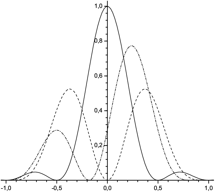
The oscillations of the differential cross section in the central region of the forward direction, $-\delta<\varphi<\delta$, are depicted on fig.1 in the cases of maximal and minimal visibilities; the pattern is almost the same for a wide range of short wavelengths, $10^{2}<d\lambda^{-1}<10^{6}$. The area under plotted lines is 0.4749701$\pm$0.0000004 for $\Phi=\Phi_{0}$, 0.4414430$\pm$0.0000010 for $\Phi=\Phi_{1\,-}$ and 0.4278549$\pm$0.0000013 for $\Phi=\frac{1}{2}\Phi_{0}$. Thus, the contribution of oscillations from the outer region, $\delta<|\varphi|<\pi$, is less than 17% of that from the central one; it is even less than 6% in the case $\Phi=\Phi_{0}$. The area under the one central peak in the case $\Phi=\Phi_{0}$ ($-\frac{1}{2}\delta<\varphi<\frac{1}{2}\delta$) is 0.4514119$\pm$0.0000002; it exceeds the area under the two peaks in the cases $\Phi=\Phi_{1\,-}$ and $\Phi=\frac{1}{2}\Phi_{0}$ ($-\delta<\varphi<\delta$). The contribution of the classical scattering to the central region is at all negligible.

We have shown that the fringe shift emerging under the influence of a magnetic vortex in the diffraction pattern in a direct scattering experiment with short-wavelength particles, see (37), is completely analogous to that in the interference pattern in a double-slit experiment, see (1). However, there are some features which are peculiar to the case of short-wavelength particles.

During the 50 years long history of the experimental verification of the AB effect (see [3]), many efforts were undertaken to ensure the impenetrability of the magnetic vortex, since the issue of penetration of particle beams into the region of the magnetic flux was the principal one to seed doubts in the verification. Perhaps, these misgivings had grounds in the case of long-wavelength particles, but, as follows from scattering theory, there is no room for them in the case of short-wavelength particles. The penetrability of the magnetic vortex does not affect the diffraction pattern (first term in (37)), only the classical reflection (given by (38)) is affected. It may seem to be somewhat paradoxical, but the AB effect with short-wavelength particles is the same for a penetrable vortex as for an impenetrable one.

The overwhelming contribution to the whole diffraction cross section comes from a narrow region, $-\delta<\varphi<\delta$, around the strictly forward direction. A gate for the strictly forward propagation of short-wavelength particles is opened for the magnetic flux equal to the flux of even number of the Abrikosov vortices, say, at $\Phi=\Phi_{0}$: more than 90% of the diffraction cross section is given by a peak centred at $\varphi=0$ and having width $\delta$. As the flux diminishes, the peak is lowered and shifted to the right. If the angular resolution is $\frac{1}{2}\delta$, then the visibility of the central point is maximal ($V=1$) at $\Phi=\Phi_{0}$, diminishing with the diminishing flux and achieving its minimum ($V=0$) at $\Phi=\Phi_{1\,-}$, see (43). Furthermore, the visibility is growing with the diminishing flux and achieves its maximum ($V=1$) for the flux equal to that of the Abrikosov vortex, at $\Phi=\frac{1}{2}\Phi_{0}$ (or odd number of the Abrikosov vortices in general). The pattern is again symmetric but with a dip in the strictly forward direction: the gate is closed. This gate effect is illustrated by fig.1 for a wide range of short wavelengths, $10^{2}<d\lambda^{-1}<10^{6}$.

Certainly, the Fraunhofer diffraction (i.e. the diffraction in almost parallel rays) is a well-known phenomenon of wave optics. Poisson was the first who predicted theoretically in 1818 a spot of brightness in the centre of a shadow of an opaque disc; the prediction was in a contradiction with the laws of geometric (ray) optics. It is curious that Poisson used his prediction as an argument to disprove wave optics which had been just developed by Fresnel: this demonstrates how unexpected and unbelievable Poisson’s result was at that time. Nevertheless, the brightness spot in the centre of the disc shadow was observed; the decisive experiments were performed by Arago and Fresnel. According to Sommerfeld [11], the diffraction on the opaque disc bears the name of Poisson and the brightness spot in the shadow centre bears the name of Arago. The same effect persists for scattering of light on an opaque sphere and other obstacles. However, in the case of obstacles in the form of a long strip or cylinder, the streak of brightness in the centre of a shadow of such obstacles might be elusive to the experimental detection: as is noted in the eminent treatise [12], it seems more likely that the measurable quantity is the classical cross section, although the details of this phenomenon depend on the method of measurement.

Almost six decades have passed from the time when this assertion was made by Morse and Feshbach, and experimental facilities have improved enormously since then. For instance, in optics, a streak of brightness in the shadow of a hair can be observed with the use of laser beams. In the present paper, we point at the circumstances when the detection of the forward diffraction peak in electron optics will be the detection of the AB effect as well. We propose to perform a scattering experiment using electrons with the wavelength of order 0.1 nm and a magnetic vortex (tiny ferromagnet or solenoid) with the diameter of order 1 $\mu$m; a distance from the vortex to the detector and that from the electron source to the vortex might be of order 100 mm.

The work was supported in part by the Ukrainian-Russian SFFR-RFBR project F40.2/108 ”Application of string theory and field theory methods to nonlinear phenomena in low-dimensional systems”.

References

- [1] Aharonov Y. and Bohm D., Phys. Rev. 115 (1959) 485.
- [2] Peshkin M. and Tonomura A., The Aharonov–Bohm Effect (Springer-Verlag, Berlin) 1989.
- [3] Tonomura A., J. Phys. A: Math. Theor. 43 (2010) 354021.
- [4] Berry M. V., Eur. J. Phys. 1 (1980) 240.
- [5] Ruijsenaars S. N. M., Ann. Phys. (N.Y.) 146 (1983) 1.
- [6] Jackiw R., Ann. Phys. (N.Y.) 201 (1990) 83.
- [7] Sitenko Yu. A. and Vlasii N. D., Europhys. Lett. 92 (2010) 60001.
- [8] Sitenko Yu. A. and Vlasii N. D., Ann. Phys. (N.Y.) 326 (2011) 1441.
- [9] Sitenko Yu. A. and Vlasii N. D., J. Phys. A: Math. Theor. 44 (2011) 315301.
- [10] Sommerfield C. M. and Minakata H., in Dynamics of Gauge Fields – Proc. TMU-Yale Symposium, edited by A. Chodos et al (Universal Academy Press, Tokyo) 2000, pp.81-90.
- [11] Sommerfeld A., Optik, Vorlesungen uber Theoretische Physik. Band IV (Wiesbaden) 1950, Kapitel V, §35.
- [12] Morse P. M. and Feshbach H., Methods of Theoretical Physics, Part II (McGraw-Hill, New York) 1953, Chapter 11, section 11.2.