Could any black holes be produced at the LHC?
Abstract
We introduce analytical quantum gravity modifications of the production cross section for terascale black holes by employing an effective ultraviolet cut off . We find the new cross sections approach the usual “black disk” form at high energy, while they differ significantly near the fundamental scale from the standard increase with respect to . We show that the heretofore discontinuous step function used to represent the cross section threshold can realistically be modeled by two functions representing the incoming and final parton states in a high energy collision. The growth of the cross section with collision energy is thus a unique signature of and number of spatial dimensions . Contrary to the classical black disk result, our cross section is able to explain why black holes might not be observable in LHC experiments while they could be still at the reach of ultra-high energy cosmic ray events.
pacs
04.60.Bc, 13.85.LgI Introduction.
Despite decades of theoretical advances and experimental progress, we are in reality no closer to a formulating a workable framework of quantum gravity – let alone finding related definitive experimental evidence – and must be content to speculate about its nature and phenomenology. This is not be only an academic exercise: probing a deeper understanding of the physical processes potentially able to unveil quantum gravity signatures would be a major breakthrough in an otherwise stagnating and discouraging situation. In this spirit, we return to the foundational connection between classical and quantum gravitation, i.e. Hawking radiation. Thanks to its robustness in the semi-classical limit, Hawking radiation is a widely accepted benchmark for any reliable theory of quantum gravity.
Unfortunately, the chances of a direct detection of the Hawking radiation are remote. Since , astrophysical black holes are too big to display any relevant quantum mechanical effects. It has alternatively been conjectured that smaller primordial black holes with masses and radii may have formed in the extreme density flucations of the early universe. With temperatures , these black holes would be so bright that we should be able to observe them, but as of now the Fermi Gamma-ray Space Telescope satellite has been unsuccessful in detecting any such evidence [1]. At even shorter length scales, one enters the domain of modern particle physics accelerators. It has been suggested, however, the possibility of a “particle black hole” is very unlikely: the energy densities required to squeeze a mass completely inside its own gravitational radius is of the order of the Planck mass [2], almost orders of magnitude higher than the LHC energy and eight orders higher than the most energetic cosmic ray ever detected [3]. It may thus seem Hawking radiation, and maybe also any hint quantum gravity, is inaccessible at least in the immediate future.
The advent of large extra spatial dimensions accessible at a fundamental scale to allows such gravitational collapse to occur for matter compressed at distances of the order of fm [4]. Despite the myriad fascinating possibilities unveiled in such scenarios, the theoretical foundations are far from being understood. Perhaps most problematic is the major limitation concerning the description of micro-black holes, in that it is impossible to correctly describe end-stage black hole evaporation in the semiclassical limit when .
Utilizing the current literature base of inadequate classical metrics, one cannot take into account the local loss of resolution which plagues the spacetime when it is probed at high energies/short scales. We thus propose a new framework to describe in an effective way the nature of a quantum spacetime and its signatures in the physics of microscopic black holes. As a preliminary step we seek to address the fundamental question: how does quantum gravity affect microscopic black hole formation?
II Black hole production.
The standard expression for the semi-classical black hole production cross section is a translation of the “hoop conjecture” [2] (for improved versions of this result and comments see [5, 6, 7, 8, 9]) a black hole is produced whenever a parton of energy hits a target with an impact parameter , i.e. smaller than the Schwarzschild radius of the effective two-body system,
| (1) |
Here, is the Heaviside step-function implemeting the constraint . Since the impact parameter is not observable, it must be integrated over to obtain the experimentally measurable production cross section:
| (2) |
We thus recover the “black disk” cross section typically found in the literature.
For a neutral, non-spinning, black hole of mass in dimensions, the horizon radius is
| (3) |
where we have introduced the higher dimensional gravitational coupling constant . We note a peculiar feature of black hole “particle” physics. As mass (energy) increases, the linear dimension of the black hole increases, in contrast to the expected behavior of normal particles whose effective scales are determined by the Compton wavelength. This unique behavior leads to a possible UV self-completion of quantum gravity [10]. By inserting equation (3) in (2), we get
| (4) |
For typical LHC energies TeV, one obtains cross sections of the order nb. Given the most recently reported LHC peak luminosity [11], this would imply that about ten black hole per second would form. In hindsight we find that, according to the black disk cross section, black holes would have formed at a non-negligible rate even in early particle physics experiments. By combining (4) with Super Proton Synchrotron (SPS) parameters and , one finds that roughly one black hole a day would have formed in 1985 [12].


The aforementioned production rate estimates have since been improved to much lower values [7, 8, 9]. These results, however, conflict with the latest experimental investigations that effectively rule out the possibility of black hole formation at the LHC [13], at least as far as the semiclassical regime is valid [14]. The weak point of the hoop conjecture is that for any black holes can be produced provided is small enough. On the contrary, we expect the black hole production channel to open only above some threshold energy. The inaccuracy of predictions due to (4) follows from the assumption that the impact parameter, , can take on aribitrary small values, which is not the case in any theory of quantum gravity where a minimal length emerges as a new fundamental constant of nature [15]. We thus have to introduce a non-vanishing lower integration limit into equation (2) to account for the breakdown of any semi-classical description of spacetime in a true quantum regime. In theories with large extra-dimensions, the constraint yields quantum gravitational excitations. Any chance to observe at least some indirect signal of quantum gravitational phenomena at LHC requires taking as the “minimal length”. Moreover, instead of demanding a cut-off in the scale size, we introduce a proper exponential suppression that drives the integral to zero faster than any power of ,
| (5) |
Integration can be carried out and gives
| (6) |
where, is the upper incomplete Gamma function defined as
| (7) |
is a smooth function with the following behavior. For we get
| (8) |
Equation (8) means that the production of arbitrary small
balck holes at low energy is zero, as we expected.
The high-energy limit of (6) is obtained by means of the
asymptotic
| (9) |
We thus reproduce the semi-classical black-disk cross section
| (10) |
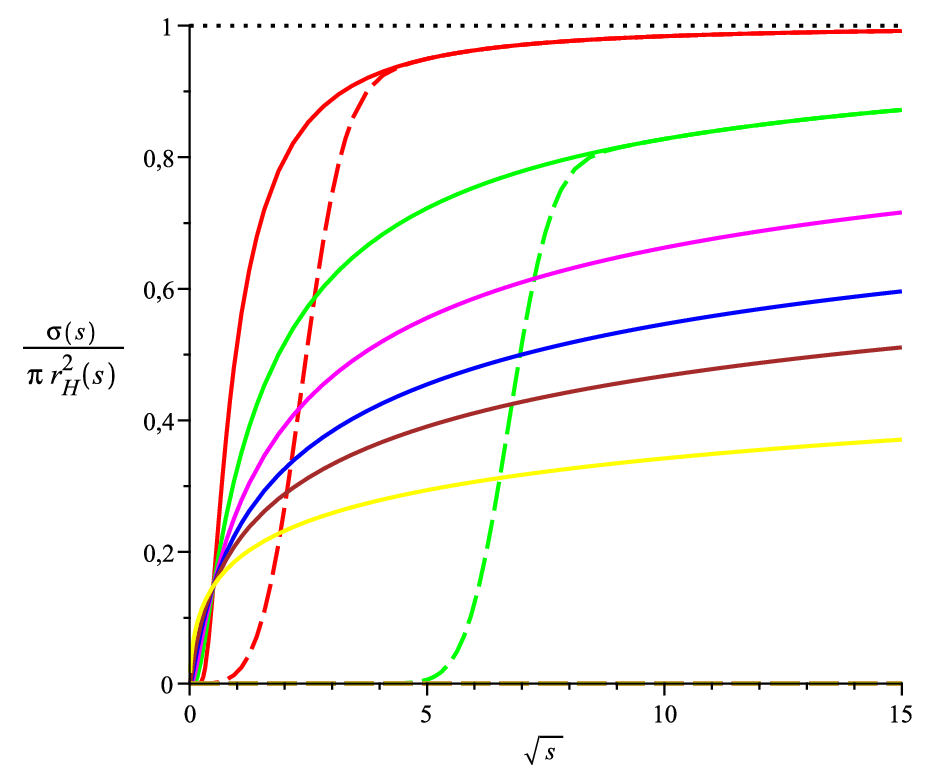
In summary, at energy above the higher dimensional unification scale, the production cross section takes on the semi-classical black-disk form, while it drops to zero very quickly for (see Fig. 1).
III Quantum gravity improved black holes.
In the following analysis, we take a further step to improve by considering that in the presence of a minimal length, whatever it is, the spacetime geometry itself is subjected to modifications. This step is motivated by the fact that semiclassical black holes offer reliable spacetime descriptions (e.g. in (3)) only when their masses are well above the fundamental mass, while they become increasingly inaccurate for energies at or just above the fundamental scale. This particular phenomenology is the goal of the present investigation. To this purpose, we recall that in recent years there have been several attempts to incorporate in black hole spacetimes the presence of quantum gravity effects through effective quantum geometries [16, 17, 18, 19, 20]. The resulting metrics (QGBHs) tend to agree on some highly desired general characters like the absence of any curvature singularity and a thermodynamically stable cooling down at the end of the evaporation [21]. In addition one finds that QGBHs do not suffer from a relevant back reaction, a fact that permits a safe employment of quantum field theory in curved space without any breakdown of the formalism. QGBHs have distinctive emission spectra: they tend to emit larger number of softer particles than semi-classical black holes with a suppressed bulk emission [22]. As a consequence QGBHs are a natural alternative to improve the scenario at hand.

A common features of such models is the introduction of a generic minimum length , which is obtained by means of a modified structure of metric coefficients
| (11) | |||
| (12) |
The function models quantum gravity corrections and is subject to the following model independent constraints (for more detailed discussions see [21]):
- i)
for the function matches its classical value, i.e., ;
- ii)
- iii)
for the function is vanishing in order to improve the curvature singularity, i.e., .
The minimum length is not fixed a priori but is assumed to be in the range , where the Planck length is the usual four-dimensional gravitational length scale and is its higher dimensional counterpart at the TeV scale. Such a minimal length bears critical importance to the production cross-section of any QGBHs that may result in high energy collisions [23].
It would be tempting to say that is given by equation (6), with replaced by . This is almost correct as it properly takes into account the role of , but ignores the existence of a minimum mass below which QGBHs do not form [24]. This minimum mass is a common feature of QGBHs and corresponds to the mass of the extremal configuration. The value of can be calculated by solving the system
in terms of . Since the creation channels opens up only for , we thus need to include this threshold condition in the cross section through a second step-function
| (13) |
Equation (13) describes the sharp opening of the production channel at the energy , but quantum mechanics introduces uncertainty and makes the step less sharp. The way the edges of the step are smoothed is determined by the “golden rule”, derived by previous investigations in noncommutative geometry, leading to regular line elements [16]. In a nut-shell, the presence of a minimal length (whatever it is its origin) translates into the replacements of Dirac delta functions into minimal width Gaussian distributions. Furthermore, since the Dirac delta is the “derivative” of the Heaviside function, it can be shown that in the framework of a minimal length a modified step function can be defined without the limit :
To derive the profile of the new cross section, we also need to determine the horizon radius by solving the equation . This can best be done by iteration on the expression
| (14) |
giving the terms
As a first step, we consider just the -th order result () and we truncate the iteration process there. For illustrative purposes we can assume In the next section we will show that, though the -th order approximation of the radius may be still acceptable, the assumption of the threshold mass becomes inadequate when quantum gravity corrections of black hole metrics are properly taken into account.
Using and at first order, we obtain
| (17) | |||||
This implies -dependent cross-section suppressions, dependent also on the presence of a mass threshold [25].
We stress the different roles of the two functions in (17). The first () comes form the hoop conjecture once the impact parameter is integrated over with a proper short-distance cut-off, while the second () describes the smooth opening of the production channel for . Generically, these can be understood to represent the outgoing (BH) and incoming (beam) states of the collision, respectively.
IV Black hole parameters/energy relations.
In the previous section we estimated the cross section by considering -th order parameters. This basically corresponds to ignoring the exact nature of quantum corrections to obtain an approximate expression for the cross section which, at the given order, turns out to be model independent. This procedure can be improved in order to obtain more accurate results. To this purpose, one has to specify a given model of QGBH and determine horizon radii and minimum masses. In doing so, one opens the possibility of discriminating among the proposed quantum gravity corrections in the class of QGBHs by comparing the resulting cross sections with experimental data.
To illustrate the procedure, we will focus on noncommutative geometry inspired black holes (NCBHs) only [16], leaving the analysis of the whole array of QGBHs in future contributions.
This choice is motivated by the following reasons. NCBHs are for now the richest family of QGBHs, since they include the higher-dimensional charged [26, 27], spinning [28] and charged-spinning [29] solutions. NCBHs are thus the only family of solutions able to describe the complete life cycle of a black hole from its formation to the end of the evaporation, a crucial necessity for phenomenological studies [30, 31]. Second, NCBHs not only capture the two primary features of QGBHs (i.e. regularity of the manifold and cooling down phase at the end of the evaporation [25]), but being a subfamily of another class of QGBHs – namely black holes in nonlocal gravity theories [20] – pave the way to model independent phenomenological conclusions.
The simplest realization of a noncommutative -dimensional spacetime due to a collapsing parton system is given by equation
| (18) | |||
| (19) |
where, to avoid notational confusion, we again indicate with the minimal length related to the size of spacetime discretization cells, while we keep for the gravitational coupling. The above line element can be equivalently identified by the function
| (20) |
in which deviations from the traditional line element are taken into account by the lower incomplete Gamma function
| (21) |
While the above metric can exhibit Killing, Cauchy and degenerate horizons, the singularity at has been removed by “spreading” the total mass energy over a region of linear size . In addition the mass spectrum is bounded from below by an extremal configuration which exists even in the case of neutral, non-spinning black holes. As expected for any QGBH, the “classical” relation (3) between horizon radii and is still valid in the high energy limit . Conversely, relevant quantum gravity deviations occur for .
The choice (20) for the profile of lets us determine the quantities and in terms of from the system
Note that (IV) can be solved only through numerical methods, whose results are given in Table 1 [25].
| 4 | 5 | 6 | 7 | 8 | 9 | |
|---|---|---|---|---|---|---|
| (TeV) | ||||||
| ( fm) |
| 4 | 5 | 6 | 7 | 8 | 9 | |
|---|---|---|---|---|---|---|
| (TeV) | ||||||
| ( fm) |
| 4 | 5 | 6 | 7 | 8 | 9 | 10 | ||
|---|---|---|---|---|---|---|---|---|
| (TeV) | ||||||||
| ( fm) |
The discrepancy between and underlines the need to properly account for black hole quantum gravity corrections beyond the rudimentary assumption .
We stress the above values depend on the definitions of the fundamental scale , which may differ for multiplicative constants (see [22] for more detailed comments on the interrelationship between them). In Table 2 and 3 we show the black hole threshold parameters according to two other major definitions of the fundamental mass. For the cases in Table 1 and 2, the minimum mass increases with spatial dimensionality, which at LHC energies would yield a virtually vanishing cross-section for . Curiously, according to the Particle Data Group notation (Table 3), we find the minimum mass decreases with spatial dimensionality for any . When we find the most promising case, corresponding to a minimum mass of roughly TeV above the maximum LHC centre-of-mass energy.
One may wonder what is the production rate related to the final formula
| (22) |
assuming the LHC’s current peak luminosity. Unfortunately, we cannot determine the horizon radius as a function of in a closed form. From the data presented in the above tables, however, we see that quantum gravity deviations are largely a function of the threshold energy. Conversely, the horizon radii are less sensitive to non-classical effects and approach the range of classical values fm even in the realm of maximum corrections, i.e. in the vicinity of the extremal configuration. This is the case irrespective of the definition of the fundamental mass, since is determined through the first equation of the system (IV).
We can show this from the equation , by considering the parton energy to contribute to both classical (-th order) and non-classical horizons, i.e. and respectively, whose ratio
| (23) |
is plotted in Figure 4. We see that the above approximation works very well not only in the high energy regime (i.e. for ), but also below the production threshold where the the function excludes the discrepancies arising from the -th order approximation of the actual non-classical horizon. It is therefore not difficult to improve the result in (17) by considering the correct threshold masses, while keeping horizon radii approximated at the -th order.
| (24) |

| = | ||||||
|---|---|---|---|---|---|---|
In the process, the production rate is mildly overestimated by virtue of the fact implies (or correspondingly ), i.e., classical horizon formation requires less energy). Consequently, use of (17) is justified under proper choice of . Tighter constraints may be obtained by simply proceeding with a more sophisticated approximation for the horizon radius, i.e., . Figure 3 demonstrates the resulting profile of cross sections for the choice of fundamental mass of Table 1. In light of the resulting rates being extremely suppressed at LHC energies for all , we can make just an example of a hypothetical collision at energies . In Table 4, we show the black hole production rate for varying energy and number of dimensions . Note the data are very sensitive to both and . For , energies above the production threshold and saturate at the black disk result. Remarkably for and energies below the production threshold , the rate is so low that the production time for a single black hole would be greater than the present age of the universe (i.e. ). Finally for , we are at energies close to the production threshold and varies dramatically with ranging from formation time scale of a second to a month. This example shows how in principle the black hole production described by (17) can also be used to indirectly determine the number of dimensions .
As a check of the huge variation of , we can write the near-threshold cross section for the production of extremal black holes. For , the leading term reads
| (25) |
which describes the approximately linear behavior of the cross section near the production threshold. The above formula can be employed to improve the results of Table 4 when considering rates at near threshold energies, i.e., for and . The corresponding values in Table 5 show that the -th order approximation can capture the orders of magnitude of productions rates even in this limit. As expected, the quantum gravity corrections of horizon radii result in slightly suppressed rates.
| = | ||||||
|---|---|---|---|---|---|---|
Estimates of for the Myers-Perry definition will not give higher production rates due to the heavier threshold masses, as is evident from Table 2. Consequently, it may be interesting to explore the case of the Particle Data Group definition, whose gravitational coupling constant turns out to be
| (26) |
Table 6 lists the production rates for the case . Despite the low threshold mass, we find that at typical LHC energies the production of black hole turns out to be improbable: at , roughly one black hole every million years would be produced in particle detectors. Due to the vicinity to the threshold mass, however, the data strongly vary and already at one finds a promising value of one black hole per month being produced. The above results can be improved by using (25), which works better near threshold and provides tighter constraints. In this case the maximum LHC beam energy significantly lowers the production rate to one black hole every million years, while at one finds a rate of approximately one black hole every 4 months. Table 7 shows the complete results that confirm how the -th order approximation can be considered valid to estimate orders of magnitude.
V Final remarks.
We have presented a first step in modeling black hole production in a post-semiclassical limit, with quantum gravity effects being introduced by a minimal length . Black production cannot occur among the variety of quantum gravity corrections we have considered, implemented below their respective threshold masses. We have provided a complete analysis of the associated cross-sections for the case of NCBHs. The related black hole production rates are highly sensitive to the value of the threshold masses, which vary non only according to the number of extra dimensions but also to the definition of the fundamental mass. Our results show that that microscopic black hole production is not a likely scenario for energies below 100 TeV with a minimum spatial dimensions. However for the case of Particle Data Group definition of the fundamental mass, we find that the LHC would be just a couple of TeV below a reasonable production rate, provided that . Our approach assumes the extra-dimensional characteristics of spacetime are those of the ADD mechanism [33], but we acknowledge that other terascale gravity models also produce similiar phenomenology, including Randall-Sundrum [34], ungravity [35], etc.. Additionally, even if we believe to have found the correct method to study these issues, our conclusions cannot be considered definitive: we still miss a complete analysis of all the remaining quantum gravity corrected black holes whose threshold masses might be at the reach of the LHC. Consequently, our result can be used by reversing the logic: instead of predicting production rates, one may determine the correct quantum gravity theory from experiment, i.e. through the value of the observed threshold mass for non-negligible production rates at LHC.
Whatever the case, even in the most pessimistic scenario such novel phenomenology is still potentially observable in ultra-high energy cosmic ray collisions.
Acknowledgements.
JM and PN would like to thank the Dipartimento di Fisica, Università di Trieste and INFN for their kind hospitality during the initial period of work on this project. This work is supported in part by the Helmholtz International Center for FAIR within the framework of the LOEWE program (Landesoffensive zur Entwicklung Wissenschaftlich-Ökonomischer Exzellenz) launched by the State of Hesse (PN), by the European Cooperation in Science and Technology (COST) action MP0905 “Black Holes in a Violent Universe” (PN) and also by a Continuing Faculty Grant from Loyola Marymount University (JM).References
- [1] http://fermi.gsfc.nasa.gov/
- [2] K. S. Thorne, Nonspherical gravitational collapse, a short review, in *J R Klauder, Magic Without Magic*, Freeman, San Francisco 1972, 231-258.
- [3] D. J. Bird et al., Phys. Rev. Lett. 71, 3401 (1993)
- [4] S. Dimopoulos and G. L. Landsberg, Phys. Rev. Lett. 87, 161602 (2001). S. B. Giddings and S. D. Thomas, Phys. Rev. D 65, 056010 (2002).
- [5] D. M. Eardley and S. B. Giddings, Phys. Rev. D 66, 044011 (2002).
- [6] S. D. H. Hsu, Phys. Lett. B 555, 92 (2003).
- [7] K. Cheung, Phys. Rev. D 66, 036007 (2002).
- [8] P. Meade and L. Randall, JHEP 0805, 003 (2008).
- [9] S. C. Park, Phys. Lett. B 701, 587 (2011).
- [10] E. Spallucci and S. Ansoldi, Phys. Lett. B 701, 471 (2011).
- [11] LHC commissioning with beam, http://lhc-commissioning.web.cern.ch/lhc-commissioning/.
- [12] B. De Raad, IEEE Trans. Nucl. Sci. 32, 1650 (1985).
- [13] V. Khachatryan et al. [CMS Collaboration], Phys. Lett. B 697, 434 (2011).
- [14] X. Calmet, W. Gong and S. D. H. Hsu, Phys. Lett. B 668, 20 (2008).
- [15] X. Calmet, M. Graesser and S. D. H. Hsu, Phys. Rev. Lett. 93, 211101 (2004).
- [16] P. Nicolini, J. Phys. A 38, L631 (2005); P. Nicolini, A. Smailagic and E. Spallucci, arXiv:hep-th/0507226; P. Nicolini, A. Smailagic and E. Spallucci, Phys. Lett. B 632, 547 (2006); T. G. Rizzo, JHEP 0609, 021 (2006); P. Nicolini and E. Spallucci, Class. Quant. Grav. 27, 015010 (2010); P. Nicolini, Phys. Rev. D 82, 044030 (2010); J. R. Mureika and P. Nicolini, Phys. Rev. D 84, 044020 (2011). R. B. Mann and P. Nicolini, Phys. Rev. D 84, 064014 (2011). P. Nicolini and G. Torrieri, JHEP 1108, 097 (2011).
- [17] L. Modesto, Phys. Rev. D 70, 124009 (2004); L. Modesto, Class. Quant. Grav. 23, 5587 (2006); L. Modesto, arXiv:1107.2403 [hep-th].
- [18] A. Bonanno and M. Reuter, Phys. Rev. D 62, 043008 (2000); A. Bonanno and M. Reuter, Phys. Rev. D 73, 083005 (2006).
- [19] R. A. Konoplya and A. Zhidenko, Phys. Rev. D 82, 084003 (2010).
- [20] L. Modesto, J. W. Moffat and P. Nicolini, Phys. Lett. B 695, 397 (2011).
- [21] V. Husain and R. B. Mann, Class. Quant. Grav. 26, 075010 (2009).
- [22] P. Nicolini and E. Winstanley, JHEP 1111, 075 (2011).
- [23] M. Bleicher, S. Hofmann, S. Hossenfelder and H. Stoecker, Phys. Lett. B 548, 73 (2002); S. Hossenfelder, M. Bleicher, S. Hofmann, J. Ruppert, S. Scherer, H. Stoecker, Phys. Lett. B575, 85-99 (2003).
- [24] S. Hossenfelder, S. Hofmann, M. Bleicher and H. Stoecker, Phys. Rev. D 66, 101502 (2002); B. Koch, M. Bleicher and S. Hossenfelder, JHEP 0510, 053 (2005).
- [25] P. Nicolini, Int. J. Mod. Phys. A 24, 1229 (2009).
- [26] S. Ansoldi, P. Nicolini, A. Smailagic and E. Spallucci, Phys. Lett. B645, 261 (2007).
- [27] E. Spallucci, A. Smailagic and P. Nicolini, Phys. Lett. B 670, 449 (2009).
- [28] A. Smailagic and E. Spallucci, Phys. Lett. B 688, 82 (2010).
- [29] L. Modesto and P. Nicolini, Phys. Rev. D 82, 104035 (2010).
- [30] R. Casadio and P. Nicolini, JHEP 0811, 072 (2008);
- [31] D. M. Gingrich, JHEP 1005, 022 (2010).
- [32] R. C. Myers, M. J. Perry, Annals Phys. 172, 304 (1986); P. Kanti, Int. J. Mod. Phys. A 19, 4899 (2004).
- [33] I. Antoniadis, N. Arkani-Hamed, S. Dimopoulos and G. R. Dvali, Phys. Lett. B 436, 257 (1998); N. Arkani-Hamed, S. Dimopoulos and G. R. Dvali, Phys. Rev. D 59, 086004 (1999).
- [34] T. Rizzo, Phys. Lett. B647, 43-48 (2007).
- [35] J. R. Mureika, Phys. Lett. B 660, 561-566 (2008).