Back Reaction from Walls

Eq. (3) can we rewritten as

with parametric solutions [12, 16]

Note that for $E=0$ Eq. (6) implies that $M\geq 0$. This equation also implies

at all times, in all cases.

The function $t_{B}(x)$ is arbitrary; it is called the ’bang time’. For $M\geq 0$, at $t=t_{B}$, i.e $\eta=0$, we have $b=0$ which represents the Big Bang singularity. Positions with $M<0$ have no Big Bang singularity but a ’bounce’ at $t=t_{B}$. We shall simplify below to the case $t_{B}\equiv 0$, i.e., uniform bang time. Note that we have chosen expanding solutions. From these we can obtain the collapsing solutions simply by changing the sign of $t$. Since in the Einstein equations only $\dot{b}^{2}$ appears they are invariant under $t\rightarrow-t$.

Of course the $\{t=$const.$\}$ hypersurfaces are not parallel to the $\{\eta=$const.$\}$ hypersurfaces, but their position depends on $x$. For fixed position $x$, Eqs. (7,8) and (12). correspond to Friedmann solutions with curvature $K=-E^{2}\leq 0$ and $M=4\pi G\rho b^{3}/3$. Note that unlike in the Friedmann case, wall solutions with $M<0$ need not be unphysical.

The parametric representation with $\eta$ is chosen in order to express the solutions in terms of elementary functions, but it is of course not necessary. For example, for $M>0$, setting

we obtain

Note that in the definition of $S$, $\left[\sinh-\rm{id}\right]^{-1}$ denotes the inverse of the function in brackets, and $\rm{id}$ is the identity function, $\rm{id}(x)=x$. One can check that $S$ solves the differential equation [18]

with initial condition $S(0)=\left(\frac{3}{4}\right)^{1/3}$. Note that this is the only regular solution, i.e solution with $S^{\prime}(0)\neq\infty$. This expression will be useful in Section 3.3.

The function $a(x,\eta)$ can be obtained from Eq. (5). For example for $M>0$ we find

(The suffix $t$ in $\partial b/\partial x$ indicates that we have to interpret $b$ as functions of $(t,x)$, not $(x,\eta)$, in this derivative.) Even if $E=0$, Eq. (4) implies that $0<M^{\prime}/E<\infty$, so that the r.h.s. of Eq. (16) is well defined. Below, we shall choose the $x$-coordinate such that $M^{\prime}/E=$constant.

Note that $M(x)$ and $E(x)$ can pass through zero so that in general different solutions from above have to be glued together at the boundary of their validity. We have checked that this gluing process can be performed in a smooth way and does not induce singularities in the scale factor $b$. However, for $M\rightarrow 0$ the scale factor $a\rightarrow\infty$. Nevertheless, we believe this to be a coordinate singularity, since, as we have checked, both, the Kretschmann scalar, $K\equiv R_{\alpha\beta\mu\nu}R^{\alpha\beta\mu\nu}$ and the scalar curvature remain finite for $M\rightarrow 0$. In our examples below we shall have $M>0$ throughout and therefore we do not encounter this problem. However, when computing $a$ from Eq. (5), one has to be careful to use the result (15) and take the limit $E\rightarrow 0$ for fixed $t$, hence also $\eta\rightarrow 0$. One cannot use (12) and (5), since for $E=0$ we have $M^{\prime}=0$ so that Eq. (5) is identically satisfied and cannot be used to obtain $a(t,x)$.

Singularities can occur when $a$, $b$ or $\rho$ become either infinite or zero. To have no singularities (apart from the Big Bang) which occurs at $t=t_{B}$, hence $b=0$, in the past light cone of every possible observer we might be interested in, we must demand that all singularities lie in the future. In more precise models, when one specifies the observer location, one can relax this condition to the one that no singularity lies within the background lightcone of the specific observer.

In general, the question of singularities depends on the choice of the functions $M(x)$ and $E(x)$. From our solutions it is clear that $b$ behaves monotonically as a function of time for fixed $x$. This is to be expected since no clustering goes on in the directions $y_{1}$ and $y_{2}$ described by this scale factor. Since we are interested in an expanding $b$, a singularity is present when the the scale factor $a$ of the $x$-direction tends to zero. From Eq. (15) we infer that for $t_{B}\equiv 0$, $a=0$ implies

It is easy to verify that the right hand side is an even positive function with minimum $4/3$ at $\eta=0$. Hence there is a singularity at some finite value of $\eta$ if the l.h.s. ever becomes larger than $4/3$ or, equivalently, if

for some value of $x$.

We now consider a simple ansatz motivated by the perturbative analysis presented in Ref. [16]. We choose

and

so that

In full generality $M^{\prime}/E=f(x)$ could be an arbitrary positive function of $x$. But we can always make a coordinate transformation to $\tilde{x}(x)$ determined by

so that with respect to the new coordinate $M^{\prime}/E=$constant. Hence we just fix the coordinate $x$ (up to a constant shift) by this choice. In addition, we have chosen uniform bang time, $t_{B}(x)\equiv 0$. This is a true restriction. With this we have reduced the three free functions of $x$ to one, $h(x)$ which defines the density profile. Furthermore, we have introduced the parameter $\epsilon$ such that for $\epsilon=0$ we reproduce the matter dominated Friedmann solution. We may also require $|h(x)|\leq 1$ so that $\epsilon$ indicates the amplitude of the perturbations. We do this in one of the examples below.

The above requirement for a singularity at some time $t\neq 0$ now reduces to $MM^{\prime\prime}<M^{\prime 2}/3$. (Strictly our derivation applies only for $M^{\prime}\neq 0$. For $M^{\prime}\propto E=0$, one sees directly from Eq. (16) that $M^{\prime\prime}\propto E^{\prime}<0$ is the necessary and sufficient condition for $a=0$ at some time $t>t_{B}$.) We have found that most interesting mass profiles satisfy this condition for some values of $x$ and therefore have singularities at some time in some places. This is not surprising but actually expected from gravitational collapse. However, when over densities become very high and we approach the collapse, pressure forces and heating become important and our simple pressure-less dust model for matter no longer holds. In order to be able to stay within the present framework, we therefore demand that such singularities be in the future and not in the past for the density profiles under consideration.

Let us consider as a first example

Then the condition for the existence of a singularity (at $t\neq 0$) becomes

which is always satisfied for some values of $x$, irrespective of $k$ and $\epsilon$. A similar behavior is expected whenever $h$ is not a convex function, but a function representing several under- and over-densities cannot be convex.

However, this is not so important for our considerations. As we have said, the requirement of singularities to be absent is mainly a technical one and it is actually sufficient not to have a singularity in the past.

Using the above expression for $a$ (for $M>0$) and the ansatz (17,19) for $M$ and $E$, we find that $a=0$ is equivalent to

Interestingly, in extremal positions of $h$, with $h^{\prime}=0$, the l.h.s. of the above expression is exactly $-1/3$. This comes from the fact that for this case $\eta=0\ \forall\ t$ and we have to replace the condition that there is no singularity before some given time $t_{0}$ by $a(t)>0$ for $t<t_{0}$ using expression (16) for $a(t)$. If $h^{\prime\prime\prime}=0$ when $h^{\prime}=0$ (as in our example) one can show that in the positions where $h$ has a maximum, hence $h^{\prime}=0$ and $h^{\prime\prime}<0$, $1+\epsilon h>0$, singularities occur first. Furthermore, when $1+\epsilon h>0$ and $h^{\prime\prime}<0$, the denominator of the l.h.s. of Eq. (20) is larger than $1$ and hence the l.h.s. becomes larger than $-1/3$. Therefore, there exists a finite value $\eta_{s}(x)$ where Eq. (20) is satisfied and $a(x,\eta_{s}(x))=0$. If, on the contrary, $1+\epsilon h>0$ and $h^{\prime\prime}>0$ the l.h.s. of Eq. (20) is smaller than $-1/3$. For positions in the vicinity of an extremum this implies that if the extremum is a minimum of $h$, the position $x$ does not encounter a singularity in the future while positions close to maxima do.

Let us study in more detail the request that the second singularity (not the big bang one) lies in the future, $t>t_{0}$. Using the expression (8) for $t$, we can rewrite the condition $a(x,\eta_{s})=0$ as

The condition $t(x,\eta_{s})>t_{0}$, for $h^{\prime}<0$ which we shall consider hence $\eta_{s}<0$ for $t(x,\eta_{s})>0$, then becomes

This equation for $\eta_{s}(x)$ can only be solved numerically. However, often we realize that the l.h.s. is smallest at small $\left|h^{\prime}\right|$ i.e. for small values of $\left|E(x)\right|$. Hence singularities will develop first in positions with small $\left|h^{\prime}\right|$. This requires also small $\left|\eta_{s}\right|$ so that we may develop the scale factor $a$ and $t$ in $\eta_{s}$. The above inequality then leads to power law relations and inserting the above expression for $E=(3/2)M^{\prime}t_{0}^{2}$ yields the constraint

The first inequality is general while for the second inequality we have chosen $h=\cos(kx)$. In Fig. 1 we plot the constraint for this case together with the condition to use the limiting solution for $E=0$, (16), (which is not necessary for our analysis) in the $\epsilon$–$\lambda$ plane, where $\lambda$ denotes the wavelength of the perturbation $\lambda=2\pi/k$.

We want to investigate whether the system of equations derived above for $z(s)$ and $D(s)$ can lead to a distance-redshift relation close to the one observed. For wall universes we consider,

For a chosen density contrast $h(x)$ we can determine $b(t,x)$ and $a(t,x)$ and solve the photon geodesic Eq. (26) for a given angle $\theta_{0}$ of the observed photon w.r.t. the $y$-plane,

We again set the initial value or the affine parameter to $0$, hence $x_{0}=x(0)$ etc.

We have investigated two choices for $M(x)$. The first is simply $M(x)=\frac{2}{9t_{0}^{2}}\left(1+\epsilon\cos(kx)\right)$ which we have already discussed before. The results for this case are shown in Fig. 2.

The result is quite striking: The deviation from the Einstein-de Sitter distance-redshift relation is very small. On the level of a few percent in the most extreme case. Much smaller than the deviation for an open (Milne) Universe or even for $\Lambda$CDM. Hence voids and walls with the chosen parameters cannot simulate the observed distance redshift relation. We have also studied different values of the parameters $(\epsilon,k)$, but all cases which are such that there is no singularity before $t_{0}$ lead to small deviation from Einstein-de Sitter. Only for wavelengths of approximately Hubble scale, $k\sim H_{0}$, where we can choose $\epsilon\sim 10^{-3}$ do the deviations become relatively large. But the density profile chosen here does not at all lead to a relation that resembles the observations.

As a second profile we consider thin, highly concentrated over-dense walls with an exponential profile:

where $\lambda=x_{i+1}-x_{i}$. In the limit $\sigma\ll\lambda$ the mean of $h\left(x\right)$ vanishes and $\text{min}_{x}h\left(x\right)=-1$. Again, we choose $\epsilon$ such that there is no singularity before $t_{0}$. The results for this profile are shown in Fig. 3.

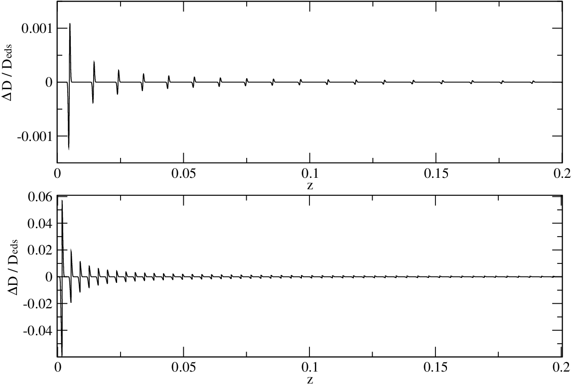
We have obtained the following result in these two examples (and other profiles which we do not present here explicitly): The modification of $D(z)$ never goes beyond the case of the open universe. We do not obtain acceleration by a series of dense walls. Even though we present here only two simple profiles, we think the conclusion is valid beyond these cases: if a photon passes through many compensated under- and over-densities in the integrated distance $D(z)$ the effect is minute as long as the time the photon spends inside a wall is much smaller than the time scale at which the gravitational potential of the wall evolves. A perturbative (first order) calculation gives a flavour of this effect. Indeed, at first order in the perturbed direction, the difference between $D(z)$ in our models and $D_{EdS}(z)$ of a matter dominated universe can be written as

where the subscripts $e$ and $o$ respectively mean that the conformal time is evaluated at the source (emission) or at the observer and expresses the perturbation of the energy density in under and over densities (see Appendix C for a derivation of the linearized result). From this expression, valid in the linear regime only, and for a periodic perturbation, it becomes clear that the deviation of $D_{L}(z)$ with respect to $D_{L}^{EdS}$ depends on the amplitude $\epsilon$ of the perturbation and on the values of the conformal time at the source and at the observer. In the case of periodic perturbations, the contributions from photon path are mostly cancelled in the integral terms. Of course in the full non-linear calculation there is no simple relation between the matter over density $h$ and the gravitational potential. In this case in principle the full non-linear Einstein equation have to be solved and Eqs. (26) and (27) govern $D_{L}(z)$.

Surprisingly, however, our non-linear simulations show that this result holds also to some extent in the non-linear regime. Note that, even though our value of $\epsilon$ is small, the over densities in the walls are large at late times, such that they develop singularities soon after today and we are deeply in the non-linear regime. While we do not have a proof that our conclusion holds in all cases, we have tested this also with other periodic wall profiles.

In Fig. 4 we show the deviations of the expansion rates with respect to the Hubble expansion in EdS universe. We note that the deviations in the unperturbed directions are small. However, in the perturbed direction these deviations can be large locally inside a wall, and they would be measurable by direct, local measurements of $H(z)$. However, they compensate when averaged over a wall thickness and do not show up in integrated quantities like $D(z)$.

Yoo et al. [18] have shown that in an LTB model every given distance–redshift relation can be mimicked by a suitable choice of the density profile. The same is true for a wall universe. For a given function $D(z)$ we can find a density profile which leads to exactly this distance–redshift relation for a photon coming in $x$-direction. First of all, for such a photon the shear vanishes for symmetry reasons and ${\cal R}$ is given by (35). To find the density profile, which is equivalent to finding $M(x)$ or $M(z)\equiv M(x(z))$ we have to solve the following coupled system of six ordinary differential equations (in principle none of the other equations couples to (41) since both, $F_{M}$ and $F_{\beta}$ do not depend on $x$ explicitly), which is very similar to the system solved in Ref. [18]:

where we have defined

In Appendix A we give the derivation of this system and the detailed expressions for $F_{M}$ and $F_{\beta}$. There, we also explain the method used to specify the initial conditions at the observer. All the constraints are fixed by requiring the system to have no critical points. Note also that $z(s)$ need not to be monotonic. If $dz/ds=0$ at a value of $s$ where $\zeta=dD/ds\neq 0$, the derivative $dD/dz$ is not well defined. This is, however, not the case of a $\Lambda$CDM Universe which we want to mimic here. We are then left with one initial condition, which we choose by requiring

i.e. the value of the Hubble rate at the observer today does not depend on direction. In Fig. 5 we show $M(x)$ as well as its derivative with respect to the $x$ coordinate, $\beta\left(x\right)$, for the solution mimicking the $\Lambda$CDM expression for $D(z)$, for $\Omega_{K}=0$, $\Omega_{m}=0.3$ and $\Omega_{DE}(z)=0.7=$constant.

In Fig. 6, we show how the luminosity distance deviates when the observer looks at photons coming in with different angles $\theta_{0}$. For $\theta_{0}=90$ degrees, we have photons traveling in $x$-direction, in this case the luminosity distance is fitted to the one of $\Lambda$CDM by solving the system of Eqs. (39-44) with the functions $M(x)$ and $\beta(x)$ shown in Fig. 5. It is interesting to remark that a given angle of $\theta_{0}\in\left[0;90\right]$ degrees at the observer corresponds to an angle at the emission $\theta_{e}>\theta_{0}$. This is a consequence of the spacetime geometry induced by the walls: due to the clustering in direction $x$, corresponding to $\theta=90^{o}$, its expansion slows down in time.

In Fig. 7, we present the density profile corrected by the isotropic expansion rate, $(1+z)^{-3}\rho(z)/\rho_{0}$, $\rho_{0}=\rho(z=0)$, obtained for our model to mimic $\Lambda$CDM luminosity distance. Finally, in Fig. 8, we plot the expansion rates in the longitudinal and transverse directions, $H_{a}=\dot{a}/a$ and $H_{b}=\dot{b}/b$. It is interesting to estimate roughly the features of the under density needed to fit $\Lambda$CDM luminosity distance. For example, if one considers the highest redshift for which we have data from supernovae, at around $z\sim 1.7$. This roughly corresponds to a size $\sim H_{0}^{-1}$. (Of course we have another data point from the CMB. The angular size of the acoustic oscillations provides an excellent measure of the angular diameter distance to the last scattering surface, $z\simeq 1090$. But this is not very relevant in our context as the Universe is to a good approximation matter dominated from $z=2$ to $z=1090$.) An under density of the size of the order of the Hubble distance is necessary to mimic $\Lambda$CDM with our walls. Moreover, we can also determine the ratio of the energy density normalized at the observer to the energy density in an Einstein-de Sitter model at $z\sim 1.7$ which is about $4$. At high redshift, $z\gtrsim 10$ the anisotropy is very small and the Universe is close to a Friedmann Universe with about 5 times the matter density obtained from local estimates.

In the previous section we have fixed $M(x)$ to reproduce the distance redshift relation of $\Lambda$CDM universe. Of course, having one free function to play with, namely $M(x)$, we expect to be able to fit one function, in our case $D(z)$. If we now proceed to another, independent observable, we shall most probably not fit it. We have done this by looking at the redshift drift, defined as the rate of change of the redshift of a co-moving source per unit of observer time. In a Friedmann Universe the redshift drift is simply

where $H(z)=H(t_{s})$ and $H_{0}$ denote the Hubble parameter at the source position at time $t_{s}$ and at the observer at the moment $t_{0}$. We have computed the corresponding function (for light rays in $x$-direction) from our solution $M(x)$. The general expression for the redshift drift of a wall Universe in $x$–direction is (see Appendix B),

Since we do not require $M_{0}=0$ as in LTB model, we can in principle have a positive redshift drift at low redshift; but we do not obtain this for our best fit profile $M(x)$ with $t_{B}(x)\equiv 0$. The result is compared with $\Lambda$CDM in Fig. 9.

Clearly the redshift drift for the two cosmologies are very different. We do have a second function to play with, the bang time $t_{B}(x)$, so that we could probably fix this observable. This has been done for LTB models in [25]. However, as it is shown there, models which have both, the same redshift distance relation and the same redshift drift as $\Lambda$CDM can be ruled out with a third observable, the kinematic Sunyaev-Zel’dovich effect which comes from the recession velocity of clusters.

References

- [1]
A. Riess et al. Astron. J. 116, 1009 (1998) [arXiv:astro-ph/9805201v1];
S. Perlmutter et al., Astrophys. J. 517, 565 (1999) [arXiv:astro-ph/9812133v1]. - [2]
R. Amanullah et al., Astrophys. J. 716, 712 (2010) [arXiv:1004.1711v1];
J. Guy et al. (2010), arXiv:1010.4743v1;
T. Holsclaw, et al., Phys. Rev. Lett. 105, 241302 (2010) [arXiv:1011.3079v1];
N. Suzuki et al. (2011), arXiv:1105.3470v1. - [3] J. Dunkley et al., Astrophys. J. 739, 52 (2011) [arXiv:1009.0866].
- [4] R. Durrer, Phil. Trans. R. Soc. A 369, 5102 (2011), doi: 10.1098/rsta.2011.0285 [arXiv:1103.5331].
- [5] C. Blake et al., Mon. Not. Roy. Ast. Soc. 418, 1725 (2011) [arXiv:1108.2637].
- [6] C. Bonvin, R. Durrer and A. Gasparini, Phy. Rev. D 73, 023523 (2006) [arXiv:astro-ph/0511183v4].
- [7]
C. Vale and M. White, Astrophys. J. 592, 699 (2003)
[arXiv:astro-ph/0303555v1];
K. Kainulainen and V. Marra, Phys. Rev. D83, 023009 (2011) [arXiv:1011.0732]. - [8] S. Räsänen, Class. Quant. Gravity 28, 164008 (2011) [arXiv:1102.0408].
- [9] G. Lemaître, 1933 Ann. Soc. Sci. Bruxelles A 53, 51 (1933); (English translation, with historical comments: Gen. Rel. Grav. 29 637, 1997).
- [10] R.C. Tolman, Proc. Nat. Acad. Sci. USA 20, 169 (1934); (reprinted, with historical comments: Gen. Rel. Grav. 29 931, 1997).
- [11]
For recent overviews see:
K. Bolejko, M-N. Célérier and A. Krasinski, Class. Quantum Grav. 28, 164002 (2011) [arXiv:1102.1449v2];
V. Marra and A. Notari, Class. Quantum Grav. 28, 164004 (2011) [arXiv:1102.1015]. - [12] P. Szekeres, Com. Math. Phys. 41, 55 (1975); Phys. Rev. D12, 2941 (1975).
- [13] A. Krasinski and K. Bolejko, Phys. Rev. D 83, 083503 (2011), [arXiv:1007.2083v2].
- [14] N. Meures and M. Bruni, MNRAS 419, 1937 (2012) [arXiv:1107.4433v2] (DOI: 10.1111/j.1365-2966.2011.19850.x).
- [15] H. Collins (2010), arXiv:1011.2046v1.
- [16] A. V. Zakharov, Soviet Physics Journal 30, 1015 (1987).
- [17] J. Plebanski and A. Krasinski, An Introduction to General Relativity and Cosmology, (Cambridge, 2006).
- [18] C.-M. Yoo, T. Kai, K. Nakao, Prog. Theor. Phys. 120, 937 (2008) [arXiv:0807.0932].
- [19] E. Komatsu et al., ApJS, 192, 18, (2011) [arXiv:1001.4538v3].
- [20] H. El-Ad and T. Piran, ApJ, 491, 421(1997) [arXiv:astro-ph/9702135v1].
- [21] P. Schneider, J. Ehlers and E.E. Falco, Gravitational Lenses, (Springer Verlag, 1992).
- [22] N. Straumann, General Relativity with Applications to Astrophysics, (Springer Verlag, 2004).
- [23] S. Seitz, P. Schneider and J. Ehlers, Class. Quantum Grav. 11, 2345 (1994) [arXiv:astro-ph/9403056v1].
- [24] V. Marra, E. W. Kolb, S. Matarrese and A. Riotto, Phys. Rev. D 76, 123004 (2007) [arXiv:0708.3622v3].
- [25] Philip Bull, Timothy Clifton, Pedro G. Ferreira, arXiv:1108.2222 (2011).
- [26] C.-M. Yoo, T. Kai, K. Nakao, Phys. Rev. D 83, 043527 (2011) [arXiv:1010.0091].
- [27] V. Perlick, Living Reviews in Relativity, 7, 9 (2004).