An Introduction to On-shell Recursion Relations

Bo Feng Affiliation: Zhejiang Institute of Modern Physics, Zhejiang University, Hangzhou, 310027, P. R. China Affiliation: Center of Mathematical Science, Zhejiang University, Hangzhou, China Mingxing Luo Affiliation: Zhejiang Institute of Modern Physics, Zhejiang University, Hangzhou, 310027, P. R. China

August 24, 2026

Abstract:

This article provides an introduction to on-shell recursion relations for calculations of tree-level amplitudes. Starting with the basics, such as spinor notations and color decompositions, we expose analytic properties of gauge-boson amplitudes, BCFW-deformations, the large $z$ -behavior of amplitudes, and on-shell recursion relations of gluons. We discuss further developments of on-shell recursion relations, including generalization to other quantum field theories, supersymmetric theories in particular, recursion relations for off-shell currents, recursion relation with nonzero boundary contributions, bonus relations, relations for rational parts of one-loop amplitudes, recursion relations in 3D and a proof of CSW rules. Finally, we present samples of applications, including solutions of split helicity amplitudes and of ${\cal N}=4$ SYM theories, consequences of consistent conditions under recursion relation, Kleiss-Kuijf (KK) and Bern-Carrasco-Johansson (BCJ) relations for color-ordered gluon tree amplitudes, Kawai-Lewellen-Tye (KLT) relations.

1 Introduction

It might be hard to over-state the importance of scattering amplitudes in particle physics and quantum field theories. They are basic building blocks of quantum field theories. Without them, quantum field theories would have lost most of their physics contents. They are indispensable in explaining almost all phenomena in particle physics. In particle physics experiments, such as those at the on-going Large Hadron Collider, scattering amplitudes are needed to make sense out of the huge mountain of experimental data. With the increasing precision of experiments and due to large contributions from gluon-loop processes, one has to calculate scattering amplitudes of many particles and to go beyond the leading-order. Leading-order calculation may tell little if anything about these experiments, neither affirmative nor negative. For many physics process, next-leading-order calculations are mandatory to understand the standard model and to delineate new physics¹¹ 1 See the Table 2 of [28] where $K$ -factors (i.e., the ratio of NLO/LO) are presented for several processes. For example, $K$ -factor of process with Higgs plus one jet is about $2.02$ .. In the Les Houches accord [28], there is the so-called wish-list for LHC experiments. The list of scattering processes are deemed particularly important and precise calculations of their amplitudes are highly desirable.

Traditionally, one relies on Feynman diagrams to calculate scattering amplitudes. Feynman diagrams provide a clear picture of physics and a systematic procedure of calculations. They are in textbooks and widely used. Calculations in quantum field theory must have been extremely difficult before their appearance. Julius Schwinger commented:²² 2 J. Schwinger, ”Quantum Electrodynamics-An Individual View,” J. Physique 43, Colloque C-8, Supplement au no. 12, 409 (1982) and ”Renormalization Theory of Quantum Electrodynamics: An Individual View,” in The Birth of Particle Physics, Cambridge University Press, 1983, p. 329. “Like the silicon chips of more recent years, the Feynman diagram was bringing computation to the masses.” Regardless the undertone, it conveyed the feeling then as well as the historical significance of Feynman diagrams.

But Feynman diagrams are not efficient in complicated calculations for high energy physics. Increasing the number of particles in a scattering, the number of Feynman diagrams increase exponentially. If gauge fields are involved, one easily encounters thousands of diagrams. For example, for pure non-Abelian gauge theory, the number of Feynman diagrams for $n$ -gluons at tree-level is given by

$n=$	$4$	$5$	$6$	$7$	$8$	$9$	$10$
	$4$	$25$	$220$	$2485$	$34300$	$559,405$	$10,525,900$

Similarly, for seven gluons at one loop, there are $227,585$ Feynman diagrams. Not only with huge number of diagrams, the expression for a single Feynman diagram can also be very complicated. For example, the three-graviton vertex has almost 100 terms. It is almost unimaginable to calculate scattering amplitudes of gravitons directly from Feynman diagrams. For gauge theories, single Feynman diagram usually depends on the gauge. Many terms cancel with each other in the process of calculation. In practice, one does not even know where to start most times. They are way beyond the ability of present-day computers. However, final results are usually simple and tidy. They are gauge invariant, as physical quantities should be.

Simply put, it is not economical and sometimes unrealistic to calculate scattering amplitudes in gauge theories via Feynman diagrams. The wish-list of LHC was thought to be a big challenge to the community. Their calculations are particularly hard and almost impossible via conventional methods. New ways have to be devised to calculate them efficiently and accurately. In last several years, with the development of various new methods, there has been tremendous progress. It has made many difficult calculations possible. In fact, most processes in the wish-list have now been calculated with the help of these methods.³³ 3 A review of recent developments of one-loop calculations can be found in [64].

As anything in scientific advancement, there are always numerous efforts before and after, sometimes heroic. It is difficult to pick up threads. One (not too arbitrary) starting point might be the formalism introduced by Xu, Zhang and Chang [170] (sometimes it is called ”Chinese magic”). Among other things, it provided a set of symbols inherited by most of late developments and proposed a new way to represent polarization vectors of massless gauge bosons. Then, neat formulas were conjectured for the so-called maximally-helicity-violating (MHV) tree-level amplitudes for gluons [142]. They were proved a few years later [21]. Despite the elegance of these formulas, no deep understanding was achieved, though a connection with string theories was pointed out.

In a seminal work [164], Witten re-expressed known scattering amplitudes in ${\cal N}=4$ super-Yang-Mills (SYM) theories in the language of twistors. The importance of MHV amplitudes⁴⁴ 4 The ${\cal N}=4$ -version of MHV amplitude is given in [137]. was emphasized. After elaborated analysis and considerations of symmetries, a duality was pointed out between ${\cal N}=4$ SYM theories and type-B topological string theories. Unfortunately, this duality does not survive beyond the leading order, as gauge bosons and gravitons do not decouple from each other in loops. Along the way, an intuitive geometrical picture was provided for scattering amplitudes in ${\cal N}=4$ SYM theories, by taking MHV amplitudes as localized on straight lines in twistor space.

Starting from the deep insight thus gained and detailed expositions of known amplitudes, a novel method (CSW) was suggested to calculate scattering amplitudes by taking MHV amplitudes as vertices, linked by scalar propagators [76]. The CSW method reproduces known results easily and generates new ones. Incidently, consistency checks of CSW rules helped to find holomorphic anomalies [77], which played an important role in later developments, such as the completion of unitarity cut method [126, 38, 37, 67, 65, 3] and direct evaluation of coefficients of one-loop amplitudes [73, 66]. It was extended to contain more physical contents and beyond the tree-level [59, 61, 72]. CSW rules were proved via several avenues[69, 150], where one of proofs will be given in late section. Compared with ordinary Feynman diagrams, CSW method has obvious advantages, with all inputs being gauge invariant on-shell amplitudes, less diagrams and much more compact expressions. However, when the number of external lines increases, expressions in intermediate calculations become extremely complex.

By analysis of relations between one-loop and tree-level amplitudes in ${\cal N}=4$ SYM theories under the infrared limit and insights from holomorphic anomalies, on-shell recursion relations was conjectured to calculate scattering amplitudes [68]. Soon after, the conjecture was proved by using fundamental properties of Feynman diagrams and the correctness of CSW method was shown [69]. This breakthrough provided an extremely powerful tool to calculate scattering amplitudes, generating new ways in calculations of multi-particle process at tree and loop levels. Starting from here, tremendous progresses have been made.

The on-shell recursion method starts with an important property of tree-level amplitudes, as they are meromorphic functions of momenta, a property due to basic physical principles such as causality. A meromorphic function is completely determined by its pole locations and corresponding residues, or cuts, which are closely related to physical quantities. For tree-amplitudes, there are only poles but no cuts. Residues are in factorized form, as products of two sub-amplitudes. Compared with Feynman diagrams or even the CSW method, on-shell recursion relations handle much less terms. All intermediate results are on-shell and gauge symmetries are automatically satisfied. Final results are very compact.

As a simple way to gauge the progress, one notices that the lowest-order of $W$ production with three jets at hadron collider could not be calculated in the early 1980’s. Recently, processes of $W,Z$ production with four jets have been computed at the 1-loop level [24, 120]. Such computations, if done by Feynman diagrams, would have required thousands of Feynman diagrams, which is obviously unrealistic. On the other hand, there are now four loop calculations of amplitudes in ${\cal N}=4$ SYM theory [31] and in ${\cal N}=8$ super-gravity [30], which was unthinkable just a few years back.

There are subtle links between on-shell recursion and the S-matrix program [139]. Both uses complexified momenta. In the S-matrix program, all components of external momenta are complexified, generating complicated complex functions of multi-variables. In on-shell recursion relations, only two external momenta are complexified in a controlled way, by introducing a complex variable. One get rather simple meromorphic functions, for which the apparatus of single-variable complex analysis is available.

This paper intends to introduce some of these progresses and ideas behind them. In particular, we intend to provided an introduction, starting from the simplest on-shell recursion relation to its various ramifications as well as sample applications. In detail, we will start with the basics in section 2, including a simple tour on spinor notations, color decompositions, and the concept of partial amplitudes in gauge theories. In section 3, we expose analytic properties of gauge-boson amplitudes, the so-called BCFW-deformation, the large $z$ -behavior of amplitudes under BCFW-deformations, and finally on-shell recursion relations of gluons. In section 4, we discuss further developments of on-shell recursion relations, including generalization to other quantum field theories, supersymmetric theories in particular, on-shell recursion relations for off-shell currents, recursion relations with nonzero boundary contributions, bonus relations, recursion relations for rational parts of one-loop amplitudes, recursion relations in 3D and a proof of CSW rules via on-shell recursion relations. In section 5, we present sample applications of on-shell recursion relations, including solutions of split helicity amplitudes and of ${\cal N}=4$ SYM theories, consequences of consistent conditions from on-shell recursion relations, Kleiss-Kuijf (KK) and Bern-Carrasco-Johansson (BCJ) relations, Kawai-Lewellen-Tye (KLT) relations and their proofs. Due to limits of space and also, limits of our abilities, many subjects are not covered. Remarks and a partial list of omissions are presented in section 6.

Now we begin our exposition.

2 Basics

In this section, we will introduce two concepts useful for simplifying calculations of scattering amplitudes, especially when they involve massless particles and fields with gauge symmetry. The first concept is spinor notation and the second one, the color decomposition.

2.1 Spinor notations

We start with a short review of spinor notations, which may not be familiar to readers. Detailed expositions can be found in [89, 132], where a Mathematica package ${\rm S@M}$ has also been developed.

Given a null momentum $k_{\mu}$ in four space-time dimensions, one may define a two-dimensional Weyl spinor $\lambda$ and an anti-spinor $\widetilde{\lambda}$ through Dirac equations

\displaystyle k_{\dot{a}a}\lambda^{a}(k)=0,~~~~\widetilde{\lambda}^{\dot{a}}(k)k_{\dot{a}a}=0~~~

(4)

where we have transformed the vector representation of the Lorentz group to bi-spinor notation through the $\sigma$ -matrices:

\displaystyle k_{\dot{a}a}\equiv k_{\mu}(\sigma^{\mu})_{\dot{a}a},~~~~\sigma^{\mu}=(1,\vec{\sigma}),~~~\dot{a},a=1,2~

(5)

It is easy to show that because $k_{\mu}\cdot k^{\mu}=\mathop{\rm det}(k_{\dot{a}a})$ , a null momentum means the matrix $k_{\dot{a}a}$ is degenerate and can be decomposed as

\displaystyle k_{\dot{a}a}=\widetilde{\lambda}_{\dot{a}}\lambda_{a},~~~

(6)

Spinor indices can be raised or lowered by anti-symmetric matrices $\epsilon^{ab}$ and $\epsilon_{ab}$ via⁵⁵ 5 We have $\epsilon^{12}=1,\epsilon_{12}=-1$ . See appendices A and B of [163] for details.

\displaystyle\lambda^{a}=\epsilon^{ab}\lambda_{b},~~~~\lambda_{a}=\epsilon_{ab}\lambda^{b}~,~~~

(7)

and similarly for dotted indices. Using $\epsilon$ we can also define Lorentz invariant inner products of two spinors or anti-spinors

\displaystyle\left\langle i|j\right\rangle\equiv\lambda^{a}_{i}\lambda_{ja},~~~~~\left[i|j\right]\equiv\widetilde{\lambda}_{i\dot{a}}\widetilde{\lambda}_{j}^{\dot{a}}~.

(8)

In standard textbooks of quantum field theories, free fermions are usually described by the Dirac equation $(\cancel{k}-m)u(p)=0$ for positive frequencies and $(\cancel{k}+m)v(p)=0$ for negative frequencies, where the $4\times 4$ $\gamma$ -matrices are taken in chiral representation. For $m\neq 0$ , there is no direct relation between these two types of solutions. When $m=0$ , positive and negative frequency solutions are identical up to normalization conventions. Solutions of definite helicity can be identified with each other as the following:

	$\displaystyle u_{\pm}(k)$	$\displaystyle=$	$\displaystyle{1\pm\gamma_{5}\over 2}u(k),~~~v_{\mp}(k)={1\pm\gamma_{5}\over 2}u(k),$		(9)
	$\displaystyle\overline{u_{\pm}(k)}$	$\displaystyle=$	$\displaystyle\overline{u(k)}{1\mp\gamma_{5}\over 2},~~~\overline{v_{\mp}(k)}=\overline{v(k)}{1\mp\gamma_{5}\over 2}$		(10)

Depending on the representation of $\gamma$ -matrices, whether Weyl or Majorana, explicit expressions of $u,v$ by $\lambda,\widetilde{\lambda}$ may be different. In our calculations, we can take the following identification⁶⁶ 6 In the literature, there are two conventions to make the identification: the QCD convention and the twistor convention. We will use the QCD convention, same as the one used in the Mathematica package ${\rm S@M}$ . The translation between these two conventions is simply $\left[~\right]_{\rm QCD}=-\left[~\right]_{\rm twistor}$ .:

	$\displaystyle\left\|i\right\rangle$	$\displaystyle\equiv$	$\displaystyle\left\|k_{i}^{+}\right\rangle=u_{+}(k_{i})=v_{-}(k_{i}),~~~~~~\left\|i\right]\equiv\left\|k_{i}^{-}\right\rangle=u_{-}(k_{i})=v_{+}(k_{i}),$		(11)
	$\displaystyle\left\langle i\right\|$	$\displaystyle\equiv$	$\displaystyle\left\langle k_{i}^{-}\right\|=\overline{u_{-}}(k_{i})=\overline{v_{+}}(k_{i}),~~~~~~\left[i\right\|\equiv\left\langle k_{i}^{+}\right\|=\overline{u_{+}}(k_{i})=\overline{v_{-}}(k_{i})$		(12)

Within these conventions, we can translate familiar expressions in Feynman diagrams to spinor notations, such as

\displaystyle\overline{u_{+}(k_{i})}\cancel{k}_{j}u_{+}(k_{l})\equiv\left[i|k_{j}|l\right\rangle,~~~\overline{u_{+}(k_{i})}\cancel{k}_{j}\cancel{k}_{m}u_{-}(k_{l})\equiv\left[i|k_{j}k_{m}|l\right]

(13)

For simplification and without confusion, we have written $k$ instead of $\cancel{k}$ at the right-handed sides of these equations. One can also demonstrate following properties of spinor variables straightforwardly:

•

Antisymmetries:

$\displaystyle\left\langle i|j\right\rangle=-\left\langle j|i\right\rangle,~~~~\left[i|j\right]=-\left[j|i\right],$ (14)

Because the anti-symmetry we have $\left\langle i|i\right\rangle=\left[i|i\right]=0$ . Also $\left\langle i|j\right]=\left[i|j\right\rangle=0$ , i.e., the inner product of a spinor and an anti-spinor vanishes.

•

Schouten identity:

\displaystyle\left|i\right\rangle\left\langle j|k\right\rangle+\left|j\right\rangle\left\langle k|i\right\rangle+\left|k\right\rangle\left\langle i|j\right\rangle=0,~~~

(15)

and similar ones for anti-spinor $\widetilde{\lambda}$ with $\left\langle~\right\rangle\to\left[~\right]$ . Notice that there are only two independent components in each spinor, so spinor $\left|i\right\rangle$ can always be expressed linearly in terms of other two spinors $\left|j\right\rangle,\left|k\right\rangle$ . The identity then follows trivially.

•

Projection operator:

\displaystyle\left|i\right\rangle\left[i\right|={1+\gamma_{5}\over 2}\cancel{k}_{i},~~~~\left|i\right]\left\langle i\right|={1-\gamma_{5}\over 2}\cancel{k}_{i},~~~\cancel{k}_{i}=\left|i\right\rangle\left[i\right|+\left|i\right]\left\langle i\right|,~~~

(16)

Using this we can calculate

\displaystyle\left\langle i|j\right\rangle\left[j|i\right]

\displaystyle=

\displaystyle\left\langle i|\cancel{k}_{j}|i\right]={\rm Tr}({1-\gamma_{5}\over 2}\cancel{k}_{i}\cancel{k}_{j})=2k_{i}\cdot k_{j}=(k_{i}+k_{j})^{2}\equiv s_{ij}~~~

(17)

from which follows the Gordon identity

\displaystyle\left\langle i|\gamma^{\mu}|i\right]=\left[i|\gamma^{\mu}|i\right\rangle=2k_{i}^{\mu},~~~

(18)

as well as Fierz rearrangement

\displaystyle\left[i|\gamma^{\mu}|j\right\rangle\left[k|\gamma_{\mu}|l\right\rangle=2\left[i|k\right]\left\langle l|j\right\rangle~~~

(19)

where we have used (18) and (17) after identifying $\left|i\right\rangle\to\left|j\right\rangle$ .

Further identities can be derived by using above results. The following are particularly useful in practical manipulations

	$\displaystyle\left\langle i\|pq\|j\right\rangle+\left\langle i\|qp\|j\right\rangle=(2p\cdot q)\left\langle i\|j\right\rangle,~~~\left\langle i\|pp\|j\right\rangle=p^{2}\left\langle i\|j\right\rangle$		(20)
	$\displaystyle\left\langle i\|p\|j\right]\left\langle j\|p\|i\right]=(2k_{i}\cdot p)(2k_{j}\cdot p)-p^{2}(2k_{i}\cdot k_{j})$		(21)

as well as

			$\displaystyle\left\langle i\|j\right\rangle\left[j\|\ell\right]\left\langle\ell\|m\right\rangle\left[m\|i\right]={\rm tr}\left({1-\gamma_{5}\over 2}\cancel{k}_{i}\cancel{k}_{j}\cancel{k}_{\ell}\cancel{k}_{m}\right)$		(22)
		$\displaystyle=$	$\displaystyle{1\over 2}\left[(2k_{i}\cdot k_{j})(2k_{\ell}\cdot k_{m})+(2k_{i}\cdot k_{m})(2k_{\ell}\cdot k_{j})-(2k_{i}\cdot k_{\ell})(2k_{j}\cdot k_{m})-4i\epsilon(i,j,\ell,m)\right]$		(23)

where $\epsilon(i,j,\ell,m)\equiv\epsilon_{\mu\nu\rho\sigma}p_{i}^{\mu}p_{j}^{\nu}p_{\ell}^{\rho}p_{m}^{\sigma}$ .

In standard Feynman rules, scattering amplitudes are expressed as functions of momenta and wave functions of external particles. For a scalar, the wave function is just one. For a fermion, we have identified $u,v$ with spinor and anti-spinor. For a vector, the wave function is a polarization vector. By (6) we have transformed null momenta to spinors and we need to do similar things to polarization vectors of gauge bosons. Using the Gordon identity (18) we can write down

\displaystyle\epsilon^{+}_{\nu}(k|\mu)={\left\langle\mu|\gamma_{\nu}|k\right]\over\sqrt{2}\left\langle\mu|k\right\rangle},~~~~~~\epsilon^{-}_{\nu}(k|\mu)={\left[\mu|\gamma_{\nu}|k\right\rangle\over\sqrt{2}\left[\mu|k\right]},~~~~~~

(24)

where $\mu$ is an arbitrary null momentum not parallel to $k$ . The choice of $\mu$ corresponds to a choice of gauge and $\sqrt{2}$ is a normalization factor. (24) can be converted into spinor notations

\displaystyle\cancel{\epsilon}^{+}(k|\mu)={\lambda_{\mu}\widetilde{\lambda}_{k}\over\sqrt{2}\left\langle\mu|k\right\rangle},~~~~~~\cancel{\epsilon}^{-}(k|\mu)={-\lambda_{k}\widetilde{\lambda}_{\mu}\over\sqrt{2}\left[\mu|k\right]},~~~~~~

(25)

Polarization vectors defined above have following properties:

$\displaystyle k\cdot\epsilon^{\pm}(k\|\mu)$	$\displaystyle=$	$\displaystyle\mu\cdot\epsilon^{\pm}(k\|\mu)=0,~~~~~\epsilon^{\pm}(\widetilde{k}\|\mu)\cdot\epsilon^{\pm}(k\|\mu)=0$	(26)
$\displaystyle 0$	$\displaystyle=$	$\displaystyle\epsilon^{+}(\widetilde{k}\|k)\cdot\epsilon^{-}(k\|\mu)=\epsilon^{+}(\widetilde{k}\|\mu)\cdot\epsilon^{-}(k\|\widetilde{k})$	(27)
$\displaystyle 0$	$\displaystyle=$	$\displaystyle\cancel{\epsilon}^{+}(k\|\mu)\left\|\mu\right\rangle=\left\langle\mu\right\|\cancel{\epsilon}^{+}(k\|\mu)=\cancel{\epsilon}^{-}(k\|\mu)\left\|\mu\right]=\left[\mu\right\|\cancel{\epsilon}^{-}(k\|\mu)$	(28)

2.1.1 Spinor notations for massive particles

Spinor formalism was first developed for massless particles, and helped to simplify calculations. However, spinor formalism can also be defined for massive particles [88, 140, 156, 155, 151]. In contrast with massless particles, the helicity of massive particles do not transform co-variantly under Lorentz transformations. Helicity eigenstates are frame dependent. This makes the formalism complicated. There are two approaches for massive spinor formalism. The first is to use massive Dirac equations to solve wave functions. The second is to decompose massive momentum $p_{\mu}$ with the help of an auxiliary null-momentum $q_{\mu}$ . These two methods are equivalent and we now present the second approach.

Using a reference null-momentum $q$ , a non-null momentum $p^{2}=-m^{2}$ can be decomposed as (using the QCD convention)

\displaystyle p_{\mu}=p^{\flat}_{\mu}-{m^{2}\over 2p\cdot q}q_{\mu}=p^{\flat}_{\mu}-{m^{2}\over\left\langle q|p|q\right]}q_{\mu}~.~~~~

(29)

Since $(p^{\flat})_{\mu}$ is massless (i.e., $(p^{\flat})^{2}=0$ ), we can find its spinor $\left|p^{\flat}\right\rangle$ and anti-spinor $\left|p^{\flat}\right]$ , which are given by

\displaystyle p^{\flat}=\left|p^{\flat}\right\rangle\left[p^{\flat}\right|+\left|p^{\flat}\right]\left\langle p^{\flat}\right|,~~~~\left|p^{\flat}\right]={\left|p|q\right\rangle\over\sqrt{\left\langle q|p|q\right]}},~~\left|p^{\flat}\right\rangle={\left|p|q\right]\over-\sqrt{\left\langle q|p|q\right]}}~.~~~

(30)

In the formula (30), the denominator $\sqrt{\left\langle q|p|q\right]}$ is for normalization. In the massless limit $m\to 0$ , spinor components return to standard ones only by rescaling with factor $t$ , i.e., $\left|p\right\rangle\to t\left|p\right\rangle$ , and $\left|p\right]\to t^{-1}\left|p\right]$ with $t=\sqrt{\left[q|p\right]/\left\langle p|q\right\rangle}$ . We can take another normalization by using $2p\cdot q=\left\langle p^{\flat}|q\right\rangle\left[q|p^{\flat}\right]$ , so

\displaystyle\left|p^{\flat}\right]={\left|p|q\right\rangle\over\left\langle p^{\flat}|q\right\rangle},~~\left|p^{\flat}\right\rangle={\left|p|q\right]\over\left[p^{\flat}|q\right]}~,

(31)

which will reduce to standard notation under the limit $m\to 0$ . With this new normalization, wave functions of fermion and anti-fermion of massive particles can be defined as follows [155, 156]

$\displaystyle u_{+}(p)$	$\displaystyle=$	$\displaystyle\left\|p^{\flat}\right\rangle+{m\over\left[p^{\flat}\|q\right]}\left\|q\right],~~~~~~u_{-}(p)=\left\|p^{\flat}\right]+{m\over\left\langle p^{\flat}\|q\right\rangle}\left\|q\right\rangle$
$\displaystyle v_{-}(p)$	$\displaystyle=$	$\displaystyle\left\|p^{\flat}\right\rangle-{m\over\left[p^{\flat}\|q\right]}\left\|q\right],~~~~~~v_{+}(p)=\left\|p^{\flat}\right]-{m\over\left\langle p^{\flat}\|q\right\rangle}\left\|q\right\rangle$
$\displaystyle\overline{u}_{-}(p)$	$\displaystyle=$	$\displaystyle\left\langle p^{\flat}\right\|+{m\over\left[q\|p^{\flat}\right]}\left[q\right\|,~~~~~~\overline{u}_{+}(p)=\left[p^{\flat}\right\|+{m\over\left\langle q\|p^{\flat}\right\rangle}\left\langle q\right\|,$
$\displaystyle\overline{v}_{+}(p)$	$\displaystyle=$	$\displaystyle\left\langle p^{\flat}\right\|-{m\over\left[q\|p^{\flat}\right]}\left[q\right\|,~~~~~~\overline{v}_{-}(p)=\left[p^{\flat}\right\|-{m\over\left\langle q\|p^{\flat}\right\rangle}\left\langle q\right\|~~~$	(32)

2.2 Color decompositions

The complication of Feynman diagrams increases dramatically when interactions with gauge fields are added. Feynman rules now contain two kinds of information: one is dynamical and the another one is group algebra carried by representations of fields. Color decompositions [133, 89] separate the information so one can deal with one thing once upon a time. We take care of the group structure first, then concentrate on the dynamical part. To see how it works, we take pure $SU(N_{c})$ gauge theory as an example.

Gluons carry adjoint representation with color indices $a=1,2,...,N^{2}_{c}-1$ , while quarks and antiquarks carry fundamental representation $N_{c}$ or anti-fundamental representation $\overline{N}_{c}$ indices, $i,\overline{j}=1,...,N_{c}$ . Generators of $SU(N_{c})$ group in the fundamental representation are traceless hermitian $N_{c}\times N_{c}$ matrices, $(T^{a})_{i}^{\overline{j}}$ , normalized according to $\mathop{\rm Tr}(T^{a}T^{b})=\delta_{ab}$ . With this normalization we have

\displaystyle f^{abc}={-i\over\sqrt{2}}{\rm Tr}(T^{a}[T^{b},T^{c}]),~~~~

(33)

thus we can use the trace structure at the right-handed side to replace $f^{abc}$ in Feynman rules. When we glue two vertices together by a propagator, we need to sum over colors

\displaystyle\sum_{a=1}^{N_{c}^{2}-1}(T^{a})_{i_{1}}^{\overline{j}_{1}}(T^{a})_{i_{2}}^{\overline{j}_{2}}=\delta_{i_{1}}^{\overline{j}_{2}}\delta_{i_{2}}^{\overline{j}_{1}}-{1\over N_{c}}\delta_{i_{1}}^{\overline{j}_{1}}\delta_{i_{2}}^{\overline{j}_{2}}~~~

(34)

which, when putting into the trace structure, is given by ”Fierz” identity (or completeness relations)

	$\displaystyle\sum_{a}{\rm Tr}(XT^{a}){\rm Tr}(T^{a}Y)={\rm Tr}(XY)-{1\over N_{c}}{\rm Tr}(X){\rm Tr}(Y)$
	$\displaystyle\sum_{a}{\rm Tr}(XT^{a}YT^{a})={\rm Tr}(X){\rm Tr}(Y)-{1\over N_{c}}{\rm Tr}(XY)~.~~~~~$		(35)

Applying (33) and (35) to all Feynman diagrams, with simple algebraic manipulations (or more intuitive double line notations [89]), tree-level amplitudes of gluons can be decomposed into the following structure⁷⁷ 7 The ${1/N_{c}}$ parts in (35) are always canceled.

\displaystyle{\cal A}_{\rm tot}(\{k_{i},\epsilon_{i},a_{i}\})

\displaystyle=

\displaystyle\sum_{\sigma\in S_{n}/Z_{n}}{\rm Tr}(T^{a_{\sigma(1)}}T^{a_{\sigma(2)}}...T^{a_{\sigma(n)}})A_{n}^{\rm tree}(\sigma(1),\sigma(2),...,\sigma(n))~~~

(36)

where group information is separated from dynamical ones. The sum is over all permutations of $n$ -particle up to cyclic ordering. The decomposition (36) is usually referred to as color decomposition, while $A_{n}^{\rm tree}$ are called partial amplitudes which contain all kinematic information.

The advantages of color decomposition are following:

•

(1) Group information and kinematic information are separated. When we change the gauge group from $SU(N_{1})$ to $SU(N_{2})$ , no calculations are needed, except those changing the fundamental representation matrix of $SU(N_{1})$ to $SU(N_{2})$ in the trace part. All partial amplitudes $A_{n}^{\rm tree}$ are same.
•

(2) The partial amplitude $A_{n}^{\rm tree}$ is the minimal gauge invariant object. It is cyclic in the sense that $A_{n}(\sigma_{1},\sigma_{2},...,\sigma_{n})=A_{n}(\sigma_{n},\sigma_{1},...,\sigma_{n-1})$ . Partial amplitudes are simpler than full amplitudes and can be calculated by using simpler color-ordered Feynman rules (see [89]). Due to color ordering, they only receive contributions from diagrams of a particular cyclic ordering of gluons. Singularities of partial amplitudes, poles and cuts (in loops), can only occur in a limited set of kinematic channels, those made out of sums of cyclically adjacent momenta. These characters make it easier to analyze partial amplitudes than full amplitudes.

Partial amplitudes have very interesting relations among themselves:

•

Color-order reversed identity

$\displaystyle A_{n}(1,2,...,n-1,n)=(-)^{n}A_{n}(n,n-1,...,2,1),~~~$ (37)
•

$U(1)$ -decoupling identity

$\displaystyle\sum_{\sigma~\rm cyclic}A(1,\sigma(2),...,\sigma(n))=0,~~~$ (38)

•

Kleiss-Kuijf relations were conjectured in [124] and proved in [87]. They are

\displaystyle A_{n}(1,\{{\alpha}\},n,\{{\beta}\})=(-1)^{n_{\beta}}\sum_{\sigma\in OP(\{{\alpha}\},\{{\beta}^{T}\})}A_{n}(1,\sigma,n)~.~~~~

(39)

The order-preserved (OP) sum is over all permutations of the set ${\alpha}\bigcup{\beta}^{T}$ , where relative orderings in ${\alpha}$ and ${\beta}^{T}$ (the reversed ordering of set ${\beta}$ ) are preserved. $n_{\beta}$ is the number of ${\beta}$ elements. For example, six gluon amplitude are related as

	$\displaystyle A(1,2,3,6,4,5)$	$\displaystyle=$	$\displaystyle A(1,2,3,5,4,6)+A(1,2,5,3,4,6)+A(1,2,5,4,3,6)$		(40)
			$\displaystyle+A(1,5,4,2,3,6)+A(1,5,2,4,3,6)+A(1,5,2,3,4,6)~.~~~$		(40)

•

Bern-Carrasco-Johansson Relations were conjectured in [33], proved in string theory by [52, 160] and in field theory by [103, 85].

The cyclic property reduces the number of independent partial amplitudes $A_{n}$ from $n!$ to $(n-1)!$ while the KK-relation reduces it to $(n-2)!$ by fixing, for example, the first and last particles to be $1$ and $n$ . The newly discovered BCJ relation enable us to reduce the number further down to $(n-3)!$ . That is, we can fix three particles at three fixed positions, for example, the first one and last two.⁸⁸ 8 In open string theory, with conformal invariance, we can fix locations of three vertexes along the boundary of disk diagram. This explains intuitively why we can fix three positions in basis. General expressions of other partial amplitudes in this basis are quite complicated and given in [33]. However, there are very simple relations, termed as “fundamental BCJ relations”, which can be used to derive all other expressions. Examples of fundamental BCJ relations are

$\displaystyle 0$	$\displaystyle=$	$\displaystyle I_{4}=A(2,4,3,1)(s_{43}+s_{41})+A(2,3,4,1)s_{41}$
$\displaystyle 0$	$\displaystyle=$	$\displaystyle I_{5}=A(2,4,3,5,1)(s_{43}+s_{45}+s_{41})$
		$\displaystyle+A(2,3,4,5,1)(s_{45}+s_{41})+A(2,3,5,4,1)s_{41}$
$\displaystyle 0$	$\displaystyle=$	$\displaystyle I_{6}=A(2,4,3,5,6,1)(s_{43}+s_{45}+s_{46}+s_{41})$	(41)
		$\displaystyle+A(2,3,4,5,6,1)(s_{45}+s_{46}+s_{41})$
		$\displaystyle+A(2,3,5,4,6,1)(s_{46}+s_{41})+A(2,3,5,6,4,1)s_{41}~~~$

where we observe the pattern of how the particle $4$ is moving from the second position to the $(n-1)$ -th position with proper kinematic factors $s_{ij}=(p_{i}+p_{j})^{2}$ .

In the above, we have only discussed color decompositions of tree-level amplitudes of pure gluons. Similar decompositions can be performed when we include matter fields like fermions or scalars, in different representations. Loop-level decompositions also exist although things will become more complicated.

2.3 Partial amplitudes in gauge theories

Having introduced notions of color decompositions and partial amplitudes in gauge theory, we now give a few examples for illustration.

On-shell gluons can have two choices of helicities (negative and positive)⁹⁹ 9 We will always define the helicity respect to outgoing momenta., so partial amplitudes can be fixed by color-ordering, helicity configuration and their momenta. The simplest example is the partial amplitudes with at most one of particle to be negative helicity and their values are

\displaystyle A_{n}^{\rm tree}(1^{\pm},2^{+},...,n^{+})=0~.

(42)

The vanishing of these partial amplitudes can be explained by using Feynman rules or supersymmetric Ward identities [89]. A less trivial example is the celebrated MHV (maximal helicity violating) amplitude, where two particles are of negative helicity and all others are of positive,

\displaystyle A_{n}(1^{+},..,i^{-},...,j^{-},...,n^{+})={\left\langle i|j\right\rangle^{4}\over\left\langle 1|2\right\rangle\left\langle 2|3\right\rangle...\left\langle n-1|n\right\rangle\left\langle n|1\right\rangle}.~~~~~~

(43)

It was conjectured in [142] and proven in [21]. In particular, the three-point partial amplitudes are

\displaystyle A_{3}(1^{-},2^{-},3^{+})={\left\langle 1|2\right\rangle^{3}\over\left\langle 2|3\right\rangle\left\langle 3|1\right\rangle},~~~A_{3}(1^{+},2^{+},3^{-})={\left[1|2\right]^{3}\over\left[2|3\right]\left[3|1\right]}.~~~

(44)

Taking the conjugation of (43) we can obtain amplitudes of two positive helicities only.

For an on-shell massless particle in spinor notation, there is an operator counting its helicity $h$

\displaystyle\left(\widetilde{\lambda}^{a}{\partial\over\partial\widetilde{\lambda}^{a}}-\lambda^{a}{\partial\over\partial\lambda^{a}}\right)A=2h_{a}A,~~{\rm given}~a~~~

(45)

Explicitly, each $\widetilde{\lambda}$ is assigned charge one and $\lambda$ charge minus one. In (43), we see that for particle $i$ of negative helicity $h_{i}=-1$ , there are four $\lambda_{i}$ in the numerator and two $\lambda_{i}$ in the denominator, thus we have $4(-1)-2(-1)=-2$ . This counting is simple, but very useful as a consistent check in practical calculations.

MHV or its conjugation $\overline{\rm MHV}$ are the simplest non-zero partial amplitudes of gluons. Calculations of other helicity configurations are not trivial, especially when the number of gluons increases. Traditional methods relying on Feynman diagrams lose their power because (1) there are too many diagrams; (2) there are too many terms in each diagram; (3) one diagram is usually not gauge invariant and many diagrams are related by gauge invariance; (4) we get gauge invariant result only when summing over certain subsets. Consequently, intermediate expressions tend to be vastly more complicated than final results, when the latter are represented properly. Feynman diagram method is simply not efficient to do such calculations.

To deal with the complexity in these calculations, many methods have been developed over the years. One of the early methods is the recursion relation of off-shell currents proposed in [21]. A recent method is the CSW method [76] and another one is to use on-shell recursion relations [68, 69]. Both methods were trigged by Witten’s twistor program [165]. A recent review of the CSW method can be found in [62]. Our focus will be on-shell recursion relations.

3 On-shell recursion relations

In this section, we show how to use general analytic properties of gluon amplitudes to derive on-shell recursion relations. Originally, they were discovered [68] by comparing infrared divergences of one-loop amplitudes with tree-level amplitudes [125, 37, 67, 152].

3.1 Analytic properties of scattering amplitudes

Naively, scattering amplitudes are functions of real variables $p_{\mu}$ . However, scattering amplitudes are fundamentally meromorphic functions of complexified momenta, as consequences of unitarity and causality. One obvious place to see these properties is in the familiar $p^{2}+i\epsilon$ prescription of propagators.

The importance of analyticity was realized long ago. The so-called S-matrix program[139], was proposed to understand scattering amplitudes (especially in strong interactions) based only on some general principles, such as Lorentz invariance, locality, causality, gauge symmetry as well as analytic properties. Different from the Lagrangian paradigm, the S-matrix program has generality as its most distinguished feature: results so obtained do not rely on any details of the theory. However, exactly because of its generality and with so little assumptions, there are not many tools available and its study is very challenging. In this article, we will see that when we combine the idea of S-matrix program and on-shell recursion relations, many important results can be derived.

One analytic property most easily seen is in the pole structure. Dictated by Feynman rules, amplitudes are constructed by connecting interaction vertices through propagators. Because of locality, obtained expressions by Feynman rules are always meromorphic functions of momenta and polarization vectors, which have pole structures when propagators are on-shell. Branch cuts and other singularities appear when these expressions are integrated over. The singularity structure of tree-level amplitudes is very simple: there are only poles.

Another well studied property is the soft limit, i.e., when all components of a momentum $k_{\mu}$ go to zero. For massive particles, on-shell conditions prevent this to happen. For massless particles, nothing prevents this. In QCD amplitudes, soft limits have universal behaviors. For example, for tree-level partial amplitudes one find

\displaystyle A_{n}^{\rm tree}(...,a,s^{+},b,...)\to{\rm Soft}(a,s^{+},b)A_{n-1}^{\rm tree}(...,a,b,...),~~~~k_{s}\to 0,~~~

(46)

where the soft or “eikonal” factor is

\displaystyle{\rm Soft}(a,s^{+},b)={\left\langle a|b\right\rangle\over\left\langle a|s\right\rangle\left\langle s|b\right\rangle}~.~~~

(47)

When momenta of external particles take certain particular values, such that one inner propagator becomes on-shell, the amplitude will factorize. When this happens, all Feynman diagrams are divided into two categories, those with and those without this particular propagator. The leading contribution comes from the first category. This can be expressed rigorously as the factorization property. A simple example is the tree-level partial amplitude of gluons when $p_{1m}^{2}\to 0$

\displaystyle A_{n}^{\rm tree}(1,2,...,n)\sim\sum_{h}A_{m+1}^{\rm tree}(1,2,..,m,-p_{1,m}^{h}){1\over p_{1m}^{2}}A_{n-m+1}^{\rm tree}(p_{1,m}^{-h},m+1,..,n),~~~

(48)

where the sum is over two physical helicities of the immediate particle $p_{1,m}$ . Under the limit $p_{1m}^{2}\to 0$ , the amplitudes at the left- and right-handed sides of the propagator become on-shell amplitudes. The leading contribution depends on products of two on-shell amplitudes.

If the number of particles involved in the factorization is equal to or more than three, we will call it a multi-particle channel. However, there is a special case called collinear channel, where only two particles are involved in the factorization. For a collinear channel, one on-shell amplitude is the three-point amplitude. As we will see presently, by quite general reasonings, the form of three-point amplitude can be uniquely fixed. Similar to the soft limit, we have an universal behavior under collinear limit, captured by the splitting function [22, 89]. One handy way (up to signs) to derive these functions is to use (44). Assuming $p_{a}=-zp_{c},p_{b}=-(1-z)p_{c}$ , the splitting function is

\displaystyle{\rm Split}_{-}^{\rm tree}(a^{+},b^{+})=A_{3}(a^{+},b^{+},c^{-}){1\over s_{ab}}\sim{\left[a|b\right]^{3}\over\left[b|c\right]\left[c|a\right]}{1\over\left\langle a|b\right\rangle\left[b|a\right]}={-\left[a|b\right]^{2}\over\left[b|c\right]\left[c|a\right]}{1\over\left\langle a|b\right\rangle}

Following from the real condition of momentum, the complex conjugation of $\lambda$ is equal to $\widetilde{\lambda}$ . So, $|\left\langle a|b\right\rangle|=|\left[a|b\right]|\sim\sqrt{s_{ab}}=\sqrt{p_{c}^{2}}$ and $|\left[a|c\right]|\sim\sqrt{(p_{a}+p_{c})^{2}}=\sqrt{(1-z)p_{c}^{2}}$ , $|\left[b|c\right]|\sim\sqrt{(p_{b}+p_{c})^{2}}=\sqrt{zp_{c}^{2}}$ . Plugging in all expressions, we have

\displaystyle{\rm Split}_{-}^{\rm tree}(a^{+},b^{+})={1\over\sqrt{z(1-z)}}{1\over\left\langle a|b\right\rangle}

(49)

Using similar method we have¹⁰¹⁰ 10 To fix the sign, see [89] for a more rigorous derivation.

\displaystyle{\rm Split}_{+}^{\rm tree}(a^{+},b^{+})=0,~~{\rm Split}_{+}^{\rm tree}(a^{+},b^{-})={(1-z)^{2}\over\sqrt{z(1-z)}}{1\over\left\langle a|b\right\rangle},~~~{\rm Split}_{-}^{\rm tree}(a^{+},b^{-})={-z^{2}\over\sqrt{z(1-z)}}{1\over\left[a|b\right]}~.

(50)

3.2 BCFW-deformation

As scattering amplitudes are understood to be meromorphic functions, they are defined over complexified momenta. Starting from a momentum configuration $(p_{1},...,p_{n})$ we can deform each of them in complex planes. However, arbitrary deformation will loose momentum conservation and bring on-shell momenta to off-shell. We are interesting in some complex deformations, such that on-shell conditions and the momentum conservation are kept. One of such deformations is the BCFW deformation.¹¹¹¹ 11 As we shall see in later sections, there can be other deformations. One example was introduced in [150] for the proof of CSW rule. It is very useful in the proof of on-shell recursion relations for gravitons [17] and has been applied in supersymmetric field theories (see, for example, [46]).

In BCFW deformation, we pick two special momenta, for example, $p_{i},p_{j}$ as reference and deform them as

\displaystyle p_{i}(z)=p_{i}+zq,~~~~p_{j}(z)=p_{j}-zq,~~~~

(51)

so momentum conservation is kept. To insist on-shell conditions for arbitrary $z$ , we require

\displaystyle q^{2}=q\cdot p_{i}=q\cdot p_{j}=0~.~~

(52)

These equations can be solved for $q$ when the dimension of space-time is four or above and the solution is in general complex. For example, we can take $q=\lambda_{i}\widetilde{\lambda}_{j}$ . In this case, we have

\displaystyle\lambda_{i}\to\lambda_{i},~~~\widetilde{\lambda}_{i}\to\widetilde{\lambda}_{i}+z\widetilde{\lambda}_{j},~~~\widetilde{\lambda}_{j}\to\widetilde{\lambda}_{j},~~~\lambda_{j}\to\lambda_{j}-z\lambda_{i}~.

(53)

This will be the mostly used deformation in this article and in the literature. It will be referred to as the $\left[i|j\right\rangle$ -deformation (it is worth to mention that $\left[i|j\right\rangle$ -deformation is different from $\left[j|i\right\rangle$ -deformation). We will also use $(i|j)$ -deformation to denote either $\left[i|j\right\rangle$ - or $\left[j|i\right\rangle$ -deformations. In the literature, the BCFW deformation is usually written in the above spinor form. However, the momentum form (51) provides another perspective.¹²¹² 12 As we will discuss later, BCFW deformation can be applied to massive theory too. In that case, the momentum form is more natural. Under this deformation, the original partial amplitude¹³¹³ 13 In this review, most times we use $A$ to denote amplitudes of gauge theory while $M$ to, amplitudes of other theories. $A(p_{i},p_{j},...)$ becomes a meromorphic function $A(z)$ of a single variable $z$ , for which powerful mathematical tools and claims are available. One of the claims is following: for an meromorphic function with only pole structures in complex plane, the knowledge of its pole locations and corresponding residues uniquely determine the function. We will see consequences of this idea shortly.

Before ending this subsection, we mention one more thing about on-shell three-point amplitudes. On-shell conditions tell that

\displaystyle 2p_{i}\cdot p_{i}=\left\langle i|j\right\rangle\left[j|i\right]=0,~~~~\forall i,j=1,2,3

(54)

so either $\left\langle i|j\right\rangle$ or $\left[i|j\right]$ must be zero. There are two possible solutions:

	$\displaystyle{\rm Solution}~(A):$		$\displaystyle\lambda_{1}\sim\lambda_{2}\sim\lambda_{3},~~~~$		(55)
	$\displaystyle{\rm Solution}~(B):$		$\displaystyle\widetilde{\lambda}_{1}\sim\widetilde{\lambda}_{2}\sim\widetilde{\lambda}_{3},~~~~$		(56)

If we insist momenta to be real, $\widetilde{\lambda}_{i}$ will be the complex conjugation of $\lambda_{i}$ . Thus we would have (55) and (56) at same time and expression (44) is zero. That is, three-point on-shell amplitudes are zero for real momenta. However, if momenta are complex, spinors $\lambda$ are independent of anti-spinors $\widetilde{\lambda}$ , so (55) and (56) have not to be true at same time. Three-point on-shell MHV-amplitudes are well defined for the case (56) and $\overline{\rm MHV}$ -amplitudes well defined for the case (55). This fact was first pointed in [164] and is crucial for on-shell recursion relations.

3.3 Large $z$ -behavior of amplitudes under BCFW-deformations

Now we apply deformation (51) to MHV amplitudes (43) with various choices of reference momenta (remembering that $i,j$ are negative helicities) and check its behavior when $z\to\infty$ :

$\displaystyle p_{i}(z)$	$\displaystyle=$	$\displaystyle p_{i}+z\lambda_{i}\widetilde{\lambda}_{j},~~~p_{j}(z)=p_{j}-z\lambda_{i}\widetilde{\lambda}_{j},\Longrightarrow\left\{\begin{array}[]{l}A(z)\to z^{-2},~~~i,j~{\rm not~nearby}\\ A(z)\to z^{-1},~~~i,j~{\rm nearby}\end{array}\right.$
$\displaystyle p_{i}(z)$	$\displaystyle=$	$\displaystyle p_{i}+z\lambda_{i}\widetilde{\lambda}_{k}(k\neq j),~~~p_{k}(z)=p_{k}-z\lambda_{i}\widetilde{\lambda}_{k},\Longrightarrow\left\{\begin{array}[]{l}A(z)\to z^{-2},~~~i,k~{\rm not~nearby}\\ A(z)\to z^{-1},~~~i,k~{\rm nearby}\end{array}\right.$
$\displaystyle p_{i}(z)$	$\displaystyle=$	$\displaystyle p_{i}+z\lambda_{k}\widetilde{\lambda}_{i}(k\neq j),~~~p_{k}(z)=p_{k}-z\lambda_{k}\widetilde{\lambda}_{i},\Longrightarrow\left\{\begin{array}[]{l}A(z)\to{z^{2}},~~~i,k~{\rm not~nearby}\\ A(z)\to{z^{3}},~~~i,k~{\rm nearby}\end{array}\right.$
$\displaystyle p_{k}(z)$	$\displaystyle=$	$\displaystyle p_{k}+z\lambda_{l}\widetilde{\lambda}_{k},~~~p_{l}(z)=p_{l}-z\lambda_{l}\widetilde{\lambda}_{k},~~k,l\neq i,j\Longrightarrow\left\{\begin{array}[]{l}A(z)\to z^{-2},~~~l,k~{\rm not~nearby}\\ A(z)\to z^{-1},~~~l,k~{\rm nearby}\end{array}\right.~~~$

Although these behaviors are observed in MHV amplitudes, they are true for all helicity configurations of gluons, as we will explain shortly [6]. They are nontrivial since individual Feynman diagram does not vanish when $z\to\infty$ in general. For gluons, no matter what helicity configuration one has, there is at least a BCFW deformation available such that when $z\to\infty$ , $A(z)\to 0$ . It is not generally true for other theories. One obvious example is the $\lambda\phi^{4}$ theory and we will come back to these theories later.

Occasionally, the large $z$ -behavior of amplitudes under BCFW-deformation can be understood by direct inspections of Feynman diagrams. In many circumstances, naive analysis of Feynman diagrams leads to wrong results, so we need a better way to deal with the problem.

We start with a simple example, where the momentum of particle $i$ of positive helicity is shifted as $p_{i}(z)=(\lambda_{i}+z\lambda_{j})\widetilde{\lambda}_{i}$ and the momentum particle $j$ of negative helicity is shifted as $p_{j}(z)=\lambda_{j}(\widetilde{\lambda}_{j}-z\widetilde{\lambda}_{i})$ , i.e., the $\left[j|i\right\rangle$ -deformation. Under these, we see $\epsilon^{+}_{i}\sim z^{-1}$ and $\epsilon_{j}^{-}\sim z^{-1}$ from (24). For cubic vertices, shifted momenta contribute a factor of $z$ , which may render the amplitude non-vanishing when $z\to\infty$ . Feynman diagrams of leading $z$ behavior are those that along the line connecting $i,j$ , only cubic vertices are attached. Here we have $m$ cubic vertices and $m-1$ propagators, thus the overall factor is ${z^{m}/z^{m-1}}\sim z$ . To get on-shell amplitudes, we need to multiply $\epsilon_{i},\epsilon_{j}$ , thus we have ${z/z^{2}}\sim z^{-1}$ , i.e., vanishing behavior when $z\to\infty$ .¹⁴¹⁴ 14 See also Peskin’s lecture [145].

Having gained some intuition in this analysis, we move to insightful arguments given in [6]. Note that momenta $p_{i}(z),p_{j}(z)\to\infty$ when $z\to\infty$ . If we take one particle as ingoing and another as outgoing, the process is as if a hard light-like particle is shooting through a soft background, created by all un-deformed particles. The process can be analyzed by working with quadratic fluctuations of the soft background.

For illustration, we analyze the amplitude of two scalars and $n$ -photons in scalar QED, by deforming momenta of two scalar particles. The Lagrangian is $L_{s}=D_{\mu}\phi^{*}D^{\mu}\phi$ , so the $z$ -dependent vertex is $\partial_{\mu}\phi^{*}A^{\mu}\phi\sim(q\cdot A)\phi^{*}\phi$ . If we choose the $q$ -light cone gauge

\displaystyle q\cdot A=0~~~

(69)

there is no vertex which contributes $z$ factors, since quartic vertices are $z$ -independent. However, each scalar propagator contributes a $z^{-1}$ . One thus arrives at

\displaystyle M_{n=2}(z)\to z^{0},~~~~M_{n>2}(z)\to z^{-1}

(70)

where the subscript $n$ means $n$ -photons. This result depends crucially on the fact that there are only two-derivatives in the Lagrangian. If terms like $D_{\mu}\phi^{*}D_{\nu}\phi F^{\mu{\alpha}}F^{\nu{\beta}}\eta_{{\alpha}{\beta}}$ are introduced, the $z$ -dependence will be totally different.

There is a very important subtle point in the gauge choice (69). This choice cannot be fulfilled in certain special cases. From the equation for the gauge choice $\Lambda(p)$

\displaystyle q_{\mu}A^{\mu}(p)+iq_{\mu}p^{\mu}\Lambda(p)=0

(71)

one sees that the $\Lambda(p)$ can be solved if and only if $q\cdot p\neq 0$ . In most Feynman diagrams, the momentum $p$ is the sum of some external momenta and for generic momentum configurations we do have $q\cdot p\neq 0$ . However, in diagrams where all other external particles interact with these two deformed particles through a single cubic vertex, one actually has $q\cdot p=0$ . In scalar QED, we do not have such particular diagrams since there is no photon self-interaction. In scalar-YM theory, we do have them, due to non-Abelian self-interactions. For this type of diagrams in scalar-YM theory, we find its $z$ -behavior directly by inspection of Feynman rules

\displaystyle M(z)\to\left\{\begin{array}[]{ll}z~~~,&(i,j)~{\rm nearby}\\ z^{0}~~,&(i,j)~{\rm not~nearby}\end{array}\right.

In gauge theories, the enhanced spin “Lorentz” symmetry plays an important role in controlling the large $z$ -behavior (plus Ward-identities). To see it, we decompose the gauge field ${\cal A}=A+a$ in terms of a background $A$ and the fluctuation $a$ . The Lagrangian becomes then

\displaystyle L_{\rm YM}=-{1\over 4}{\rm tr}D_{[\mu}a_{\nu]}D^{[\mu}a^{\mu]}+{i\over 2}{\rm tr}[a_{\mu},a_{\nu}]F^{\mu\nu}+(D_{\mu}a^{\mu})^{2}=-{1\over 4}{\rm tr}D_{\mu}a_{\nu}D^{\mu}a^{\mu}+{i\over 2}{\rm tr}[a_{\mu},a_{\nu}]F^{\mu\nu}~~~

(75)

where $(D_{\mu}a^{\mu})^{2}$ has been added to fix the gauge of $a$ . In (75) only the first term can potentially have ${\cal O}(z)$ -vertices and dominate the large $z$ -behavior. But the first term has also the enhanced spin symmetry, i.e., a Lorentz transformation acting only on the $\nu$ -indices of $a_{\nu}$ alone while $D_{\mu}$ is untouched. To make it clear, we rewrite the Lagrangian as

\displaystyle L_{\rm YM}=-{1\over 4}{\rm tr}\eta^{ab}D_{\mu}a_{a}D^{\mu}a_{b}+{i\over 2}{\rm tr}[a_{a},a_{b}]F^{ab}~~~

(76)

where the second term break the enhanced spin symmetry explicitly. With this symmetry argument, the amplitude will be of the general form

\displaystyle M^{ab}=(c_{1}z+c_{0}+c_{-1}{1\over z}+...)\eta^{ab}+A^{ab}+{1\over z}B^{ab}+...

(77)

where $A^{ab}$ comes from the second term of (76) and is antisymmetric. To get on-shell amplitudes, one needs to contract $M^{ab}$ with polarization vectors $\epsilon_{i},\epsilon_{j}$ . Using the Ward-identity

\displaystyle(p_{i}+zq)_{a}M^{ab}\epsilon_{jb}=0,~~~~~\Longrightarrow q_{a}M^{ab}={-1\over z}p_{ia}M^{ab}\epsilon_{jb}

(78)

For example, with $h_{i}=-,h_{j}=+$ , we have $\epsilon_{i}^{-}(z)=\epsilon_{j}^{+}(z)=q$ , thus

	$\displaystyle M^{-+}$	$\displaystyle=$	$\displaystyle\epsilon_{ia}^{-}M^{ab}\epsilon_{jb}^{+}=q_{a}M^{ab}q_{b}={-1\over z}p_{ia}\left[(c_{1}z+c_{0}+c_{-1}{1\over z}+...)\eta^{ab}+A^{ab}+{1\over z}B^{ab}+...\right]q_{b}$		(79)
		$\displaystyle=$	$\displaystyle{-1\over z}p_{ia}A^{ab}q_{b}\to{1\over z}$		(79)

where $p_{i}\cdot q=0$ has been used. With $h_{i}=+,h_{j}=-$ , we have $\epsilon_{i}^{+}(z)=q^{*}-zp_{j}$ , $\epsilon_{j}^{-}(z)=q^{*}+zp_{i}$ , so

	$\displaystyle M^{+-}$	$\displaystyle=$	$\displaystyle\epsilon_{ia}^{+}M^{ab}\epsilon_{jb}^{-}=(q^{}-zp_{j})\left[(c_{1}z+c_{0}+c_{-1}{1\over z}+...)\eta^{ab}+A^{ab}+{1\over z}B^{ab}+...\right](q^{}+zp_{i})$		(80)
		$\displaystyle\to$	$\displaystyle z^{3}$		(80)

We can do better by using the $q$ -light-cone gauge to eliminate ${\cal O}(z)$ -vertices up to a unique set of diagrams, which can exist only when $i,j$ are nearby. If $i$ and $j$ are separated by at least two insertions of $F^{ab}$ , we will have $M^{-+},M^{--},M^{++}\to z^{-2}$ and $M^{+-}\to z^{2}$ .

For pure gravity theory¹⁵¹⁵ 15 The large $z$ behavior of gravity is not so easy to discuss using Feynman diagrams directly, see several discussions in [60, 74, 17]., we again expand around the background and add a de-Donder gauge fixing term. We then have

\displaystyle L=\sqrt{-g}\left[{1\over 4}g^{\mu\nu}\nabla_{\mu}h^{\beta}_{\alpha}\nabla_{\nu}h^{\alpha}_{\beta}-{1\over 8}g^{\mu\nu}\nabla_{\mu}h^{\alpha}_{\alpha}\nabla_{\nu}h^{\beta}_{\beta}-h_{{\alpha}{\beta}}h_{\mu\nu}{1\over 2}R^{{\beta}\mu{\alpha}\nu}+{1\over 2}g^{\mu\nu}\partial_{\mu}\phi\partial_{\nu}\phi\right]

(81)

where $\phi$ is the dilaton field and $R_{\mu\nu}=0$ by background field equation. With field redefinition $h_{\mu\nu}\to h_{\mu\nu}+g_{\mu\nu}\phi\sqrt{2\over D-2}$ , $\phi\to{1\over 2}g^{\mu\nu}h_{\mu\nu}+\phi\sqrt{D-2\over 2}$ , the Lagrangian is simplified to

\displaystyle L=\sqrt{-g}\left[{1\over 4}g^{\mu\nu}g^{{\alpha}\rho}g^{{\beta}\sigma}\nabla_{\mu}h_{{\alpha}{\beta}}\nabla_{\nu}h_{\rho\sigma}-{1\over 2}h_{{\alpha}{\beta}}h_{\mu\nu}R^{{\beta}\mu{\alpha}\nu}+{1\over 2}g^{\mu\nu}\partial_{\mu}\phi\partial_{\nu}\phi\right]

(82)

We will drop the dilaton field in later discussions. To make two copies of enhanced spin symmetry,¹⁶¹⁶ 16 Actually $e=\widetilde{e}$ and $\omega=\widetilde{\omega}$ , but two copies make things transparent. we introduce the left vielbein $e$ and the right vielbein $\widetilde{e}$ , so that

\displaystyle h_{\mu\nu}=e^{a}_{\mu}\widetilde{e}^{\widetilde{a}}_{\nu}h_{a\widetilde{a}},~~~~\nabla_{\alpha}h_{\mu\nu}=e^{a}_{\mu}\widetilde{e}^{\widetilde{a}}_{\nu}D_{\alpha}h_{a\widetilde{a}}=e^{a}_{\mu}\widetilde{e}^{\widetilde{a}}_{\nu}\left(\partial_{\alpha}h_{a\widetilde{a}}+\omega^{b}_{{\alpha}a}h_{b\widetilde{a}}+\widetilde{\omega}^{\widetilde{b}}_{{\alpha}\widetilde{a}}h_{a\widetilde{b}}\right)

(83)

The final Lagrangian is given by

\displaystyle L=\sqrt{-g}\left[{1\over 4}g^{\mu\nu}\eta^{ab}\widetilde{\eta}^{\widetilde{a}\widetilde{b}}D_{\mu}h_{a\widetilde{a}}D_{\nu}h_{b\widetilde{b}}-{1\over 2}h_{a\widetilde{a}}h_{b\widetilde{b}}R^{ab\widetilde{a}\widetilde{b}}\right]

(84)

Taking the light-cone gauge $\omega_{ab}^{+}=\widetilde{\omega}_{\widetilde{a}\widetilde{b}}^{+}=g^{++}=g^{+i}=0$ and $g^{+1}=1$ , the general pattern of two-leg off-shell amplitude is

\displaystyle M^{a\widetilde{a}b\widetilde{b}}=cz^{2}\eta^{ab}\widetilde{\eta}^{\widetilde{a}\widetilde{b}}+z(\eta^{ab}\widetilde{A}^{[\widetilde{a}\widetilde{b}]}+A^{[ab]}\widetilde{\eta}^{\widetilde{a}\widetilde{b}})+A^{[ab][\widetilde{a}\widetilde{b}]}+(\eta^{ab}\widetilde{B}^{\widetilde{a}\widetilde{b}}+B^{ab}\widetilde{\eta}^{\widetilde{a}\widetilde{b}})+{1\over z}C^{ab\widetilde{a}\widetilde{b}}~~~

(85)

where square brackets denote anti-symmetrization of indices. The form (85) manifestly has the form of “squaring” a Yang-Mills theory, similar to the KLT relation $M_{\rm gravity}\sim M_{\rm gauge}\times M_{\rm gauge}$ . Using Ward-identity to replace $q_{a}M^{a\widetilde{a},b\widetilde{b}}\epsilon_{j,b\widetilde{b}}=-z^{-1}p_{ia}M^{a\widetilde{a},b\widetilde{b}}\epsilon_{j,b\widetilde{b}}$ , so that

	$\displaystyle M^{--,--}(z)$	$\displaystyle=$	$\displaystyle\epsilon_{i,a\widetilde{a}}^{--}M^{a\widetilde{a},b\widetilde{b}}\epsilon_{j,b\widetilde{b}}^{--}={1\over z^{2}}p_{ia}p_{i\widetilde{a}}M^{a\widetilde{a},b\widetilde{b}}(q^{}_{b}+zp_{ib})(q^{}_{\widetilde{b}}+zp_{i\widetilde{b}})$		(86)
		$\displaystyle=$	$\displaystyle{1\over z}C^{ab\widetilde{a}\widetilde{b}}p_{ia}p_{i\widetilde{a}}p_{ib}p_{i\widetilde{b}}\to{1\over z}$		(86)

In fact, with a little extra work one can show that $C^{ab\widetilde{a}\widetilde{b}}$ is the sum of terms antisymmetric in $(ab)$ and in $(\widetilde{a}\widetilde{b})$ . The leading scaling behavior is actually $z^{-2}$ .

In short, the large $z$ -behavior of amplitudes under the BCFW-deformation is a nontrivial intrinsic property of a theory. The understanding of this property provides a new way to calculate on-shell amplitudes, as to be discussed now.

3.4 On-shell recursion relations of gluons

We now derive on-shell recursion relations [68, 69] for partial amplitudes.¹⁷¹⁷ 17 There are also efforts to understand on-shell recursion relations by using Feynman diagrams [92, 162]. The starting point is the meromorphic function $A(z)$ of a single complex variable $z$ , obtained by picking up a pair of particles $(i,j)$ and doing the BCFW-deformation (51), with proper choice of $q$ such that $A(z)\to 0$ when $z\to\infty$ . From (3.3), one sees that no matter which helicity configuration $(i,j)$ is, there is at least one choice of $q$ satisfying the vanishing requirement of $A(z)$ at infinity of $z$ .

The function $A(z)$ has a simple single-pole structure for general momenta, due to propagators of the form

\displaystyle{1\over(p+p_{i}(z))^{2}}={1\over(p+p_{i})^{2}+z(2q\cdot(p+p_{i}))}~~~~

(87)

where $p_{j}$ is not inside the momenta sum $p$ . For any function $A(z)$ has only single poles at finite $z$ , we can consider the following contour integration

\displaystyle I

\displaystyle=

\displaystyle\oint{dz\over z}A(z)~~~

(88)

where the contour is a big enough circle including all finite poles. The integration can be evaluated in two different ways. The first is to deform the contour to the infinity and we denote the result as the boundary contribution $B$ . If $A(z)\to 0$ as $z\to\infty$ , the boundary contribution $B=0$ . The second is to deform the contour to encircle all finite poles, so we have

\displaystyle I

\displaystyle=

\displaystyle A(z=0)+\sum_{z_{\alpha}}{\rm Res}\left({A(z)\over z}\right)_{z_{\alpha}}

(89)

where nonzero finite poles come from propagators of the form (87) and $A(z=0)$ is the tree-level partial amplitude we intend to calculate. Identifying both evaluations, one has

\displaystyle A(z=0)=B-\sum_{z_{\alpha}}{\rm Res}\left({A(z)\over z}\right)_{z_{\alpha}}~.~~~

(90)

Now the key is to calculate residues, which can be obtained via the factorization property (48). The residue depends on products of two on-shell sub-amplitudes,

\displaystyle\left({A(z)\over z}\right)_{z_{\alpha}}=-\sum_{h=\pm}A_{L}(p_{i}(z_{\alpha}),p^{h}(z_{\alpha})){1\over P_{\alpha}^{2}}A_{R}(-p^{-h}(z_{\alpha}),p_{j}(z_{\alpha}))

(91)

where one sums over two helicities of the inner on-shell propagator. Putting all together we obtain a recursion relation for the gluon amplitude

\displaystyle A_{n}

\displaystyle=

\displaystyle\sum_{z_{\alpha},h=\pm}A_{L}(p_{i}(z_{\alpha}),p^{h}(z_{\alpha})){1\over p_{\alpha}^{2}}A_{R}(-p^{-h}(z_{\alpha}),p_{j}(z_{\alpha}))+B~~~~

(92)

where $B$ will be zero if the proper deformation makes $A(z)\to 0$ when $z\to\infty$ .

For color-ordered partial amplitudes, allowed propagators always have momenta of the form $p_{kt}=p_{k}+p_{k+1}+p_{k+2}+...+p_{t}$ . Thus, the number of terms in the recursion formula depends on the choice of pair $(i,j)$ . When $i,j$ are adjacent, one has minimum number of terms. For example, taking $(n-1,n)$ as the BCFW-deformation pair with $q=\lambda_{n-1}\widetilde{\lambda}_{n}$ , we have

			$\displaystyle A_{n}(1,2,...,(n-1)^{-},n^{+})$		(93)
		$\displaystyle=$	$\displaystyle\sum_{i=1}^{n-3}\sum_{h=+,-}\left(A_{i+2}({\hat{n}},1,2,...,i,-{\hat{p}}^{h}_{n,i}){1\over p^{2}_{n,i}}A_{n-i}(+{\hat{p}}^{-h}_{n,i},i+1,...,n-2,{\hat{n-1}})\right),~~~$		(93)

where

$\displaystyle p_{n,i}$	$\displaystyle=$	$\displaystyle p_{n}+p_{1}+\ldots+p_{i},$
$\displaystyle\widehat{p}_{n,i}$	$\displaystyle=$	$\displaystyle p_{n,i}+{p_{n,i}^{2}\over\left\langle n-1\|p_{n,i}\|n\right]}\lambda_{n-1}\tilde{\lambda}_{n},$
$\displaystyle\widehat{p}_{n-1}$	$\displaystyle=$	$\displaystyle p_{n-1}-{p_{n,i}^{2}\over\left\langle n-1\|p_{n,i}\|n\right]}\lambda_{n-1}\tilde{\lambda}_{n},$
$\displaystyle\widehat{p}_{n}$	$\displaystyle=$	$\displaystyle p_{n}+{p_{n,i}^{2}\over\left\langle n-1\|p_{n,i}\|n\right]}\lambda_{n-1}\tilde{\lambda}_{n}.~~~$	(94)

Shown in Figure 1 is a pictorial representation of (93). Although it is obvious that $\widehat{p}_{n,i}$ is null, it is not so easy to read out its spinor and anti-spinor components. After some algebra, it can be shown that

\displaystyle\left|\widehat{p}_{n,i}\right\rangle={\alpha}\left|p_{n,i}|n\right],~~~~\left|\widehat{p}_{n,i}\right]={\beta}\left|p_{n,i}|n-1\right\rangle,~~~{\alpha}{\beta}={1\over\left\langle n-1|p_{n,i}|n\right]}~~~

(95)

which are very useful in practical calculations.

Refer to caption — Figure 1: Pictorial representation of the recursion relation (93). Note that the difference between terms in the two sums is the helicity assignment of the internal line.

We now demonstrate the usefulness of on-shell recursion relations in the example of six gluons. It is the simplest case where non-MHV amplitudes show up. We will calculate three helicity configurations: $(---+++)$ , $(++-+--)$ , $(+-+-+-)$ .

We start with $A(1^{-},2^{-},3^{-},4^{+},5^{+},6^{+})$ , which is actually the simplest. The reference gluons are chosen to be $\hat{3}$ and $\hat{4}$ . There are three possible configurations of external gluons, as shown in Figure 2. The middle graph vanishes. In the other two graphs, only one helicity configuration of the internal gluon gives a nonzero answer. We are left with only two graphs to evaluate. Moreover, the two graphs are related by a flip of indices and a complex conjugation. Therefore, only one computation is needed.

Let us work out the details of Figure 2(a). It is the product of two MHV amplitudes and a propagator,

\displaystyle\left(\left\langle 2~\hat{3}\right\rangle^{3}\over\left\langle\hat{3}~\hat{p}\right\rangle\left\langle\hat{p}~2\right\rangle\right){1\over t_{2}^{[2]}}\left({\left\langle 1~\hat{p}\right\rangle^{3}\over\left\langle\hat{p}~\hat{4}\right\rangle\left\langle\hat{4}~5\right\rangle\left\langle 5~6\right\rangle\left\langle 6~1\right\rangle}\right)~~~

(96)

where $t_{i}^{[k]}=\sum_{j=i}^{i+k-1}p_{j}$ . Note that

\displaystyle\lambda_{\hat{3}}

\displaystyle=

\displaystyle\lambda_{3},~~~\lambda_{\hat{4}}=\lambda_{4}-{t_{2}^{[2]}\over\left\langle 3~2\right\rangle[2~4]}\lambda_{3},~~~\left\langle\bullet~\hat{p}\right\rangle=-{\left\langle\bullet|2+3|4\right]\over[\hat{P}~4]}.

(97)

(96) can straightforwardly be simplified to

\displaystyle{\left\langle 1|2+3|4\right]^{3}\over[2~3][3~4]\left\langle 5~6\right\rangle\left\langle 6~1\right\rangle t_{2}^{[3]}\left\langle 5|3+4|2\right]}.~~~

(98)

Finally, performing the flip: $i\to i+3$ and the complex conjugation: $\left\langle~~\right\rangle\leftrightarrow[~~]$ in (98), we obtain the expression for Figure 2(c). Adding them up and factoring out a common term, we get

\displaystyle A(1^{-},2^{-},3^{-},4^{+},5^{+},6^{+})={1\over\left\langle 5|3+4|2\right]}\left({\left\langle 1|2+3|4\right]^{3}\over[2~3][3~4]\left\langle 5~6\right\rangle\left\langle 6~1\right\rangle t_{2}^{[3]}}+{\left\langle 3|4+5|6\right]^{3}\over[6~1][1~2]\left\langle 3~4\right\rangle\left\langle 4~5\right\rangle t_{3}^{[3]}}\right).

(99)

Actually, this expression was first found [152] by taking a collinear limit of a seven-gluon amplitude in [35].

For the other two helicity configurations, there are three terms. Specifically,

$\displaystyle A(1^{+},2^{+},3^{-},4^{+},5^{-},6^{-})$	$\displaystyle=$	$\displaystyle{[2~4]^{4}\left\langle 5~6\right\rangle^{3}\over[2~3][3~4]\left\langle 6~1\right\rangle t_{2}^{[3]}\left\langle 1\|2+3\|4\right]\left\langle 5\|3+4\|2\right]}$	(100)
		$\displaystyle+{\left\langle 3\|1+2\|4\right]^{4}\over\left\langle 1~2\right\rangle\left\langle 2~3\right\rangle[4~5][5~6]t_{1}^{[3]}\left\langle 1\|2+3\|4\right]\left\langle 3\|1+2\|6\right]}$
		$\displaystyle+{[1~2]^{3}\left\langle 3~5\right\rangle^{4}\over[6~1]\left\langle 3~4\right\rangle\left\langle 4~5\right\rangle t_{3}^{[3]}\left\langle 5\|3+4\|2\right]\left\langle 3\|4+5\|6\right]}~,~~~$

from configurations $(2,\hat{3}|\hat{4},5,6,1)$ , $(1,2,\hat{3}|\hat{4},5,6)$ , and $(6,1,2,\hat{3}|\hat{4},5)$ , respectively; and

$\displaystyle A(1^{+},2^{-},3^{+},4^{-},5^{+},6^{-})$	$\displaystyle=$	$\displaystyle{[1~3]^{4}\left\langle 4~6\right\rangle^{4}\over[1~2][2~3]\left\langle 4~5\right\rangle\left\langle 5~6\right\rangle t_{1}^{[3]}\left\langle 6\|1+2\|3\right]\left\langle 4\|2+3\|1\right]}$	(101)
		$\displaystyle+{\left\langle 2~6\right\rangle^{4}[3~5]^{4}\over\left\langle 6~1\right\rangle\left\langle 1~2\right\rangle[3~4][4~5]t_{3}^{[3]}\left\langle 6\|4+5\|3\right]\left\langle 2\|3+4\|5\right]}$
		$\displaystyle+{[1~5]^{4}\left\langle 2~4\right\rangle^{4}\over\left\langle 2~3\right\rangle\left\langle 3~4\right\rangle[5~6][6~1]t_{2}^{[3]}\left\langle 4\|2+3\|1\right]\left\langle 2\|3+4\|5\right]}~,~~~$

from configurations $(1,\hat{2}|\hat{3},4,5,6)$ , $(6,1,\hat{2}|\hat{3},4,5)$ , and $(5,6,1,\hat{2}|\hat{3},4)$ , respectively. In $A(1^{+},2^{-},3^{+},4^{-},5^{+},6^{-})$ , the second and the third terms can be obtained from the first by shifting all indices: $i\to i+2$ and $i\to i+4$ .

The recursion relation (92) expresses any amplitude in terms of amplitudes of fewer gluons but of generic different helicity configurations. It is hard to find closed-form solutions of (92) for general $n$ .¹⁸¹⁸ 18 In [91], compact analytical formulae for all tree-level color-ordered gauge theory amplitudes involving any number of external gluons and up to three massless quark-anti-quark pairs have been given by projecting the known expressions [94] for ${\cal N}=4$ SYM theory. The result for ${\cal N}=4$ SYM theory will be presented shortly.

However, there is a set of amplitudes that closes under the recursion procedure. In other words, a given amplitude in the set is determined by amplitudes in the set only. They are amplitudes of the form

\displaystyle A_{p,q}=A(1^{-},2^{-},\ldots,p^{-},(p+1)^{+},\ldots,(p+q)^{+})~~~

(102)

for any integers $p\geq 1$ and $q\geq 1$ , which will be referred to as split helicity amplitudes [70]. Let us apply the recursion formula (92) to (102) by taking $p^{-}$ and $(p+1)^{+}$ to be reference gluons. Only two terms appear and they are

	$\displaystyle((p-1),\hat{p}~\|~\widehat{p+1},\ldots,(p+q),1,\ldots,(p-2)),$
	$\displaystyle((p+3),\ldots,(p+q),1,\ldots,\hat{p}~\|~\widehat{p+1},(p+2)).$		(103)

The first term depends on $A_{p-1,q}\times A_{2,1}$ , while the second on $A_{p,q-1}\times A_{1,2}$ . Thus the set of amplitudes (102) closes under (92).

Denote the number of terms in $A_{p,q}$ as $N_{p,q}$ . It satisfies also a recursion relation: $N_{p,q}=N_{p-1,q}+N_{p,q-1}$ with boundary conditions $N_{2,q}=1,~\forall q\geq 1$ and $N_{p,2}=1,~\forall p\geq 1$ . This relation can be solved by a binomial coefficient: $N_{p,q}=C_{p+q-4}^{p-2}$ . A general solution for split helicity amplitudes will be provided in section 5.

4 On-shell recursion relations: further developments

The derivation of gluon on-shell recursion relations depends on the following observations: (1) for tree-level amplitudes, there are only single poles from propagators under BCFW-deformation; (2) the residues of single poles are determined by factorization properties; (3) with proper choice of deformation, the boundary contribution is zero. Among these observations, the first two are universal for all local quantum field theories. One naturally generalizes on-shell recursion relations to other quantum field theories, by carefully taking care of boundary contributions.¹⁹¹⁹ 19 For more general discussions, see for example, [6, 81]. These include, gravity theory [60, 74, 17], gluons coupled with fermions²⁰²⁰ 20 In [130], applications to fermions in fundamental representations were emphasized, as they are of particular importance in LHC physics. [129, 130, 147, 140], gluons coupled with massive scalars [10], gluons coupled with massive vector bosons [11], quiver gauge theories [141], gluons coupled with Higgs particles [25], one-loop integral coefficients [29, 58], one-loop rational part [40, 41, 42], supersymmetric theories [57, 5], other dimensions [82, 113], off-shell currents [108], etc. These generalizations have forms similar to (92), of expressions in term of sub-amplitudes $A_{L},A_{R}$ and helicity sums of middle propagators. But there are new features in different situations and some of them will be presented in later subsections. Before going to explicit generalizations, we discuss two issues.

When we deal with massive particles instead of massless ones, we need a null momentum $q$ satisfying conditions (52) [10] to define deformation (51). In the massless case, one simply has $q=\lambda_{i}\widetilde{\lambda}_{j}$ or $q=\lambda_{j}\widetilde{\lambda}_{i}$ . For massive momenta, things are more complicated. For the case where $p_{i}^{2}=0$ and $p_{j}^{2}\neq 0$ , one finds

\displaystyle q_{{\alpha}\dot{\alpha}}=\left|i\right\rangle(\left|p_{j}|i\right\rangle)=\lambda_{i{\alpha}}p_{j\dot{\alpha}{\beta}}\lambda^{\beta}_{i},~~~~{\rm or}~~~q_{{\alpha}\dot{\alpha}}=\left|i\right](\left|p_{j}|i\right])=\widetilde{\lambda}_{i\dot{\alpha}}p_{j{\alpha}\dot{\beta}}\widetilde{\lambda}^{\dot{\beta}}_{i}~.~~~

(104)

For the case $p_{i}^{2}\neq 0$ , $p_{j}^{2}\neq 0$ , we first construct two null momenta by linear combinations $\eta_{\pm}=(p_{i}+x_{\pm}p_{j})$ with $x_{\pm}=\left(-2p_{i}\cdot p_{i}\pm\sqrt{(2p_{i}\cdot p_{j})^{2}-4p_{i}^{2}p_{j}^{2}}\right)/2p_{j}^{2}$ . The solution can then be written as

\displaystyle q=\lambda_{\eta_{+}}\widetilde{\lambda}_{\eta_{-}},~~~~~{\rm or}~~~~~~q=\lambda_{\eta_{-}}\widetilde{\lambda}_{\eta_{+}}~.~~~

(105)

When fermion propagators are involved, extra care should be taken for signs. In sub-amplitudes $A_{L},A_{R}$ , we usually take all momenta to be out-coming (or in-going),. Depending on the choice of the momentum $p$ of the middle propagator, we will have either $A_{L}(p,..)A_{R}(-p,...)$ or $A_{L}(-p,...)A_{R}(p,..)$ . The definition of spinors of negative momentum $-p$ is not unique. One option is to take $\lambda_{p}=\lambda_{-p}$ , $\widetilde{\lambda}_{p}=-\widetilde{\lambda}_{-p}$ .

Notice that the propagator used in the on-shell recursion relation is always the scalar-like ${i/p^{2}}$ . This form is natural for scalars or vectors, but not for fermions. The familiar fermion propagator is ${i\cancel{p}/p^{2}}$ . In the sum $\sum_{\pm}A_{L}(p)A_{R}(-p)$ , one term will yield $\left|p\right]\left\langle-p\right|=\left|p\right]\left\langle p\right|$ , while the other $\left|p\right\rangle\left[-p\right|=-\left|p\right\rangle\left[p\right|$ . However, $\left|p\right\rangle\left[p\right|+\left|p\right]\left\langle p\right|=\cancel{p}$ , according to identity (16). Thus to reproduce the desired $\cancel{p}$ , there must be a relative sign between the two terms in the sum. More details about signs can be found in the Appendix of [114].

Now we are going to present several generalizations. Each has its unique points. The generalization to supersymmetric theories groups fermions and bosons together as well as different helicity states. The generalization to off-shell current and amplitudes with un-vanishing boundary contributions extend the scope of applications. Bonus relation provides more relations other than on-shell recursion relations. The rational part of one-loop amplitudes has double poles, which do not exist in tree-level amplitudes. The generalization to three dimensional space-time will have the feature that propagators are quadratic function of $z$ . Finally, the proof of CSW rule uses different analytic deformation comparing to BCFW-deformation.

4.1 Generalization to supersymmetric theories

In a supersymmetric theory, bosonic and fermionic fields can be grouped together in super-multiplets with the help of Grassmannian coordinates. External lines of supersymmetric scattering amplitudes can be represented in super-fields. To get scattering amplitudes of component fields, we just need to expand Grassmannian coordinates.

To make the discussion more concrete, we focus on the ${\cal N}=4$ theory. First, we can write down a super-wave-function of Grassmann variables $\eta^{A}$ ( $A=1,2,3,4$ is for R-symmetry $SU(4)$ of ${\cal N}=4$ theory)

	$\displaystyle\Phi(p,\eta)$	$\displaystyle=$	$\displaystyle G^{+}(p)+\eta^{A}\Gamma_{A}(p)+\frac{1}{2}\eta^{A}\eta^{B}S_{AB}(p)+\frac{1}{3!}\eta^{A}\eta^{B}\eta^{C}\epsilon_{ABCD}\bar{\Gamma}^{D}(p)$		(106)
			$\displaystyle\ +\frac{1}{4!}\eta^{A}\eta^{B}\eta^{C}\eta^{D}\epsilon_{ABCD}G^{-}(p)\,,~~~~$		(106)

which incorporates all on-shell states of the theory. The $\mathcal{N}=4$ version of MHV tree amplitudes is [137]

\displaystyle{\cal A}^{\rm MHV}_{n}(\lambda,\tilde{\lambda},\eta)=\frac{\delta^{(4)}(\sum_{i}\lambda_{i}\widetilde{\lambda}_{i})\,\delta^{(8)}(\sum_{i=1}^{n}\ \lambda_{i}^{\alpha}\,\eta^{A}_{i})}{\left\langle 1\,2\right\rangle\left\langle 2\,3\right\rangle\ldots\left\langle n\,1\right\rangle}~.~~

(107)

The combination $\sum_{i=1}^{n}\ \lambda_{i}^{\alpha}\,\eta^{A}_{i}$ is called the “super-momentum” and the appearance of $\delta^{(8)}$ is dictated by ${\mathcal{N}}=4$ supersymmetry to impose super-momentum conservation, just as $\delta^{(4)}$ ensures ordinary momentum conservation. To get amplitudes for component fields, we expand (107) and read out corresponding Grassmannian components. For example,

\displaystyle\delta^{(8)}(\sum_{i=1}^{n}\ \lambda_{i}^{\alpha}\,\eta^{A}_{i})=\delta^{4}(\sum_{i<j}\left\langle i|j\right\rangle\eta_{i}^{A}\eta_{j}^{A})\to\left\langle i|j\right\rangle^{4}\prod_{A=1}^{4}\eta_{i}^{A}\eta_{j}^{A}

(108)

$\prod_{A=1}^{4}\eta_{i}^{A}\eta_{j}^{A}$ corresponds to the amplitude of all particles are gluons of positive helicity, except $i,j$ of negative helicity. If all particles are gluons of positive helicity except that $i$ is a gluon of negative helicity, $j$ a fermion of positive spin and $k$ a fermion of negative spin, we need the term $\prod_{A=1}^{4}\eta_{i}^{A}\eta_{j}^{1}\prod_{B=2}^{4}\eta_{k}^{B}$ . It is given by

\displaystyle\delta^{4}(\sum_{i<j}\left\langle i|j\right\rangle\eta_{i}^{A}\eta_{j}^{A})\to\left\langle i|k\right\rangle^{3}\left\langle i|j\right\rangle\eta_{i}^{1}\eta_{j}^{1}\prod_{A=2}^{4}\eta_{i}^{A}\eta_{j}^{A}

(109)

where we need to be careful about signs when exchanging Grassmanian variables.

As one sees, the helicity information is now hidden in $\eta$ ’s. One thus needs to generalize the BCFW-deformation to the following

\displaystyle\lambda_{i}(z)=\lambda_{i}+z\lambda_{j},~~~\widetilde{\lambda}_{j}(z)=\widetilde{\lambda}_{j}-z\widetilde{\lambda}_{j},~~~\eta_{j}(z)=\eta_{j}-z\eta_{i},~~~~

(110)

so both momentum and super-momentum conservations are kept. The large $z$ behavior of super-amplitudes is universal. It is $z^{-1}$ when $i,j$ are nearby and $z^{-2}$ when $i,j$ are not nearby. The on-shell recursion relation in ${\cal N}=4$ theory is [57, 5]

\displaystyle\mathcal{A}=\sum_{\rm split~{\alpha}}\int d^{4}\eta_{P_{i}}\mathcal{A}_{L}(p_{i}(z_{\alpha}),p_{{\alpha}}(z_{\alpha}))\frac{1}{p_{{\alpha}}^{2}}\mathcal{A}_{R}(p_{j}(z_{\alpha}),-p_{{\alpha}}(z_{\alpha}))\,.~~~

(111)

where the integration is over Grassmanian variables and the sum is over all possible inner propagators.

There is one nice thing in (111). All helicity configurations are packed together as one-object, the recursion relation is closed. That is, all sub-amplitudes are of the same type, just like the case of split helicity amplitudes. Thus it is possible to solve the recursion relation explicitly, as we will see in the next section.

4.2 Recursion relations for off-shell currents

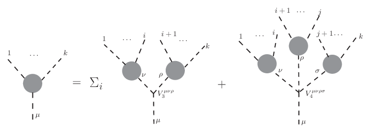
Before the discovery of on-shell recursion relations, an off-shell recursion relation (also known as Berends-Giele recursion relation) for gluon current was proposed [21] based directly from Feynman diagrams, where all external lines except one are on-shell. The off-shell recursion relation of current $J^{\mu}$ is²¹²¹ 21 The factor ${-i}/{p_{1,k}^{2}}$ indicates that the gluon propagator is in the Feynman gauge.

	$\displaystyle J^{\mu}\left(1,2,...,k\right)$	$\displaystyle=$	$\displaystyle\frac{-i}{p_{1,k}^{2}}\left[\sum_{i=1}^{k-1}V_{3}^{\mu\nu\rho}\left(p_{1,i},p_{i+1,k}\right)J_{\nu}\left(1,...,i\right)J_{\rho}\left(i+1,...,k\right)\right.$		(112)
			$\displaystyle\left.+\sum_{j=i+1}^{k-1}\sum_{i=1}^{k-2}V_{4}^{\mu\nu\rho\sigma}J_{\nu}\left(1,...,i\right)J_{\rho}\left(i+1,...,j\right)J_{\sigma}\left(j+1,...,k\right)\right]$		(112)

where $p_{i,j}=p_{i}+p_{i+1}+\cdots+p_{j}$ . $p_{1,k}$ is the momentum of the off-shell line and vertices are

	$\displaystyle V_{3}^{\mu\nu\rho}\left(p,q\right)$	$\displaystyle=$	$\displaystyle\frac{i}{\sqrt{2}}\left(\eta^{\nu\rho}\left(p-q\right)^{\mu}+2\eta^{\rho\mu}q^{\nu}-2\eta^{\mu\nu}p^{\rho}\right)$
	$\displaystyle V_{4}^{\mu\nu\rho\sigma}$	$\displaystyle=$	$\displaystyle\frac{i}{2}\left(2\eta^{\mu\rho}\eta^{\nu\rho}-\eta^{\mu\nu}\eta^{\rho\sigma}-\eta^{\mu\sigma}\eta^{\nu\rho}\right)~.~~~~$		(113)

Recursion (112) starts with $J^{\mu}(1)=\epsilon^{\pm\mu}(p_{1})$ , which is the current with only one on-shell gluon. Shown in Fig 4 is a graphic presentation of (112). As we have mentioned, the off-shell recursion relation (112) has been used to prove the validity of Parke-Taylor formula of MHV-amplitudes.

Different from gauge invariant on-shell amplitudes, $J^{\mu}(1,2,...,k)$ is gauge dependent, as there is a line which is not on-shell and not contracted with a physical polarization vector. The gauge freedom arises in several places. The first is in the choice of null reference momentum to define polarization vectors of external on-shell gluons

\displaystyle\epsilon_{i\mu}^{+}=\frac{\left\langle r_{i}|\gamma_{\mu}|p_{i}\right]}{\sqrt{2}\left\langle r_{i}|p_{i}\right\rangle},~~~~~\epsilon_{i\mu}^{-}=\frac{\left[r_{i}|\gamma_{\mu}|p_{i}\right\rangle}{\sqrt{2}\left[r_{i}|p_{i}\right]}~~~~~

(114)

where $p_{i}$ is the momentum of the $i$ -th gluon and $r_{i}$ is its null reference momentum. The second is in the choice of gluon propagator and we always use the Feynman gauge. To deal with the gauge dependence, we need to define two more polarization vectors²²²² 22 The $\epsilon^{L},\epsilon^{T}$ have different mass-dimensions from those of $\epsilon^{\pm}$ . This can be fixed by proper factors such as $\sqrt{p_{i}^{2}}$ when $p_{i}^{2}\neq 0$ . For our purpose, this factor does not matter and we will use (114) for simplicity.

\displaystyle\epsilon_{\mu}^{L}=p_{i},~~~~\epsilon_{\mu}^{T}={\left\langle r_{i}|\gamma_{\mu}|r_{i}\right]\over 2p_{i}\cdot r_{i}}~~~

(115)

Using Fierz rearrangements (19), one sees that

	$\displaystyle 0$	$\displaystyle=$	$\displaystyle\epsilon^{+}\cdot\epsilon^{+}=\epsilon^{+}\cdot\epsilon^{L}=\epsilon^{+}\cdot\epsilon^{T}=\epsilon^{-}\cdot\epsilon^{-}=\epsilon^{-}\cdot\epsilon^{L}=\epsilon^{-}\cdot\epsilon^{T}=\epsilon^{T}\cdot\epsilon^{T}=\epsilon^{L}\cdot\epsilon^{L}$
	$\displaystyle 1$	$\displaystyle=$	$\displaystyle\epsilon^{+}\cdot\epsilon^{-}=\epsilon^{L}\cdot\epsilon^{T}~~~$		(116)

These four $\epsilon$ vectors form a basis of the four-dimension space-time and we have

\displaystyle g_{\mu\nu}=\epsilon_{\mu}^{+}\epsilon_{\nu}^{-}+\epsilon_{\mu}^{-}\epsilon_{\nu}^{+}+\epsilon_{\mu}^{L}\epsilon_{\nu}^{T}+\epsilon_{\mu}^{T}\epsilon_{\nu}^{L}~~~

(117)

which is the numerator of the gluon propagator in Feynman gauge.

Now we are ready to write down the on-shell recursion relation for $J^{\mu}$ [108]. Since $J^{\mu}(1,2,...,k)$ has $k$ on-shell gluons, we can take a pair of on-shell gluons to do the BCFW-deformation and write down the corresponding on-shell recursion relation. The boundary behavior under the $\left[i|j\right\rangle$ -deformation will be same as those of on-shell amplitudes. That is, $z^{-1}$ for helicity configurations $(-,+),(+,+),(-,-)$ and $z^{3}$ for the helicity configuration $(+,-)$ .²³²³ 23 The boundary behavior is in fact more subtle. For example, if $(i,j)$ are not nearby, we will have ${1/z^{2}}$ behavior for $(-,+),(+,+),(-,-)$ . For our purpose, naive counting is enough.^,²⁴²⁴ 24 The boundary behavior of off-shell particles has also been analyzed in [54] directly by using Feynman diagrams. The off-shell line causes no extra problem.

Taking $(i,j)=(1,k)$ , one has

	$\displaystyle J^{\mu}\left(1,2,...,k\right)$	$\displaystyle=$	$\displaystyle\sum_{i=2}^{k-1}\sum_{h,\widetilde{h}}\left[A\left(\widehat{1},...,i,\widehat{p}^{h}\right)\cdot\frac{1}{p_{1,i}^{2}}\cdot J^{\mu}\left(-\widehat{p}^{\widetilde{h}},i+1,...,\widehat{k}\right)\right.$
	$\displaystyle+J^{\mu}\left(\widehat{1},...,i,\widehat{p}^{h}\right)$		$\displaystyle\left.\cdot\frac{1}{p_{i+1,k}^{2}}\cdot A\left(-\widehat{p}^{\widetilde{h}},i+1,...,\widehat{k}\right)\right],~~(h,\widetilde{h})=(+,-),(-,+),(L,T),(T,L)~~$		(118)

There are several things in (118) which need to be mentioned. First, since $J^{\mu}\left(1,2,...,k\right)$ is gauge dependent, all reference momenta in sub-currents on the right-handed side of (118) must be the same as those on the left-handed side of (118). Secondly, for the on-shell momentum $\widehat{p}$ on the right-handed side of (118), we must sum over all four polarization vectors in (114) and (115) (not just vectors in (114)). As we see in (117), they decompose the $g_{\mu\nu}$ factor of gluon propagator in Feynman gauge. We can neglect vectors in (115) for on-shell amplitudes, because $\epsilon^{L}=\widehat{p}$ and when all other particles are on-shell and with physical polarizations, $\widehat{p}\cdot A=0$ by virtue of Ward identities. For configurations $(h,\widetilde{h})=(L,T),(T,L)$ in (118), we have either $\widehat{p}\cdot A_{L}=0$ or $\widehat{p}\cdot A_{R}=0$ , so we are left with only two familiar helicity configurations in recursion relations for on-shell amplitudes. For current $J^{\mu}$ , we do not have $\epsilon^{L,T}\cdot J\neq 0$ , thus we can not neglect the sum over $(h,\widetilde{h})=(L,T),(T,L)$ . However, we will show that usually these two terms vanish by a special choice of gauge. Also we can use Ward identities to simplify calculations. For example, for the $(h,\tilde{h})=(T,L)$ configuration, the second term in (118) vanishes due to Ward identity

\displaystyle A\left(-\widehat{p}^{L},i+1,...,\widehat{k}\right)=-\widehat{p}^{L}_{\mu}\cdot M^{\mu}\left(i+1,...,\widehat{k}\right)=0

(119)

The starting point is of course the two-point off-shell currents of various helicity configurations

$\displaystyle J^{\mu}\left(1^{-},2^{+}\right)$	$\displaystyle=$	$\displaystyle\frac{1}{\sqrt{2}s_{12}}\left(\frac{[r_{1}2]\langle 1r_{2}\rangle}{[r_{1}1]\langle r_{2}2\rangle}\left(1-2\right)^{\mu}+\frac{[2r_{1}]\langle 21\rangle}{[r_{1}1]\langle r_{2}2\rangle}\langle r_{2}\|\gamma^{\mu}\|2]+\frac{[12]\langle r_{2}1\rangle}{[r_{1}1]\langle r_{2}2\rangle}[r_{1}\|\gamma^{\mu}\|1\rangle\right)$	(120)
$\displaystyle J^{\mu}\left(1^{+},2^{+}\right)$	$\displaystyle=$	$\displaystyle\frac{1}{\sqrt{2}s_{12}}\left(\frac{[12]\langle r_{2}r_{1}\rangle}{\langle r_{1}1\rangle\langle r_{2}2\rangle}\left(1-2\right)^{\mu}+\frac{[21]\langle r_{1}2\rangle}{\langle r_{1}1\rangle\langle r_{2}2\rangle}\langle r_{2}\|\gamma^{\mu}\|2]+\frac{[21]\langle r_{2}1\rangle}{\langle r_{1}1\rangle\langle r_{2}2\rangle}\langle r_{1}\|\gamma^{\mu}\|1]\right)~~$	(121)
$\displaystyle J^{\mu}\left(1^{-},2^{T}\right)$	$\displaystyle=$	$\displaystyle\frac{1}{\sqrt{2}s_{12}}\left(-\frac{\left\langle 12\right\rangle\left[2r_{1}\right]}{\left[r_{1}1\right]}\left(1+2\right)^{\mu}+\frac{\left\langle 12\right\rangle\left[21\right]}{\left[r_{1}1\right]}\left\langle 1\|\gamma^{\mu}\|r_{1}\right]\right)~~$	(122)
$\displaystyle J^{\mu}\left(1^{+},2^{T}\right)$	$\displaystyle=$	$\displaystyle\frac{1}{\sqrt{2}s_{12}}\left(\frac{\left\langle r_{1}2\right\rangle\left[21\right]}{\left\langle r_{1}1\right\rangle}\cdot\left(1+2\right)^{\mu}-\frac{\left\langle 12\right\rangle\left[21\right]}{\left\langle r1\right\rangle}\left\langle r\|\gamma^{\mu}\|1\right]\right)~~$	(123)

where the gauge dependence of each on-shell gluon is kept. Now we use these building blocks to calculate one example of three on-shell gluons.

The example of $J^{\mu}\left(1^{-},2^{+},3^{+}\right)$

Under the $\left[i|j\right\rangle$ -deformation, the recursion relation is

	$\displaystyle J^{\mu}\left(1^{-},2^{+},3^{+}\right)$	$\displaystyle=$	$\displaystyle J^{\mu}\left(\widehat{1}^{-},\widehat{p}^{+}\right)\cdot\frac{1}{s_{23}}\cdot A\left(-\widehat{p}^{-},\widehat{2}^{+},3^{+}\right)+J^{\mu}\left(\widehat{1}^{-},\widehat{p}^{-}\right)\cdot\frac{1}{s_{23}}\cdot A\left(-\widehat{p}^{+},\widehat{2}^{+},3^{+}\right)$		(124)
			$\displaystyle+J^{\mu}\left(\widehat{1}^{-},\widehat{p}^{L}\right)\cdot\frac{1}{s_{23}}\cdot A\left(-\widehat{p}^{T},\widehat{2}^{+},3^{+}\right)+J^{\mu}\left(\widehat{1}^{-},\widehat{p}^{T}\right)\cdot\frac{1}{s_{23}}\cdot A\left(-\widehat{p}^{L},\widehat{2}^{+},3^{+}\right)$		(124)

Here there is only one cut $s_{23}$ due to color-ordering. The second term in (124) vanishes if all helicities are positive while the fourth term vanishes due to Ward identity. Using a general reference null-momentum $q$ for the internal gluon $\widehat{p}$ , the first and third terms are given as

	$\displaystyle J^{\mu}\left(\widehat{1}^{-},\widehat{p}^{+}\right)\cdot\frac{1}{s_{23}}\cdot A\left(-\widehat{p}^{-},\widehat{2}^{+},3^{+}\right)$
	$\displaystyle=\frac{1}{\sqrt{2}s_{\widehat{1}\widehat{p}}}\left[-\frac{\left\langle\widehat{1}q\right\rangle\left[\widehat{p}\widehat{2}\right]}{\left[\widehat{2}\widehat{1}\right]\left\langle q\widehat{p}\right\rangle}\left(\widehat{1}-\widehat{p}\right)^{\mu}-\frac{\left\langle\widehat{p}\widehat{1}\right\rangle\left[\widehat{2}\widehat{p}\right]}{\left\langle q\widehat{p}\right\rangle\left[\widehat{2}\widehat{1}\right]}\left\langle q\|\gamma^{\mu}\|\widehat{p}\right]+\frac{\left\langle\widehat{1}q\right\rangle\left[\widehat{p}\widehat{1}\right]}{\left[\widehat{2}\widehat{1}\right]\left\langle q\widehat{p}\right\rangle}\left\langle\widehat{1}\|\gamma^{\mu}\|\widehat{2}\right]\right]\cdot\frac{1}{s_{23}}\cdot\frac{\left[\widehat{2}3\right]^{3}}{\left[\widehat{2}\widehat{p}\right]\left[\widehat{p}3\right]}$
	$\displaystyle J^{\mu}\left(\widehat{1}^{-},\widehat{p}^{L}\right)\cdot\frac{1}{s_{23}}\cdot A\left(-\widehat{p}^{T},\widehat{2}^{+},3^{+}\right)$
	$\displaystyle=\frac{1}{\sqrt{2}s_{\widehat{1}\widehat{p}}}\left[-\frac{\left\langle\widehat{1}\widehat{p}\right\rangle\left[\widehat{p}\widehat{2}\right]}{\left[\widehat{2}\widehat{1}\right]}\left(\widehat{1}+\widehat{p}\right)^{\mu}+\frac{\left\langle\widehat{1}\widehat{p}\right\rangle\left[\widehat{p}\widehat{1}\right]}{\left[\widehat{2}\widehat{1}\right]}\left\langle\widehat{1}\|\gamma^{\mu}\|\widehat{2}\right]\right]\cdot\frac{1}{s_{23}}\cdot\frac{\left\langle\widehat{p}\widehat{1}\right\rangle\left\langle q\widehat{1}\right\rangle\left[\widehat{2}3\right]}{\left\langle\widehat{p}q\right\rangle\left\langle\widehat{1}\widehat{2}\right\rangle\left\langle\widehat{1}3\right\rangle}~~~$		(125)

On can numerically check that the result is $q$ -gauge invariant. For this helicity configuration, a good gauge choice is $r_{1}=p_{2}$ , $r_{2}=r_{3}=p_{1}$ . When we choose $q=p_{1}$ in (125), it is easy to see that many terms vanish. Plugging all these in, we get immediately

\displaystyle J^{\mu}\left(1^{-},2^{+},3^{+}\right)=\frac{\left[32\right]\left\langle 1|\gamma^{\mu}{k}_{123}|1\right\rangle}{\sqrt{2}s_{12}s_{123}\left\langle 23\right\rangle}

(126)

In formula (118) we have taken a pair of on-shell particles to do the BCFW-deformation. However, one can also take an on-shell particle and the off-shell leg to do the BCFW-deformation and write down corresponding recursion relation. More details can be found in [108].

4.3 Recursion relations with nonzero boundary contributions

The original version of on-shell recursion relation was constructed and proved under the assumption that the boundary contribution $B$ in (90) vanishes. This is indeed the case if $A(z)$ vanishes as $z\to\infty$ .²⁵²⁵ 25 More accurately, if $A(z)$ has the expansion $A(z)=\sum_{i}{c_{i}/(z-z_{i})}+B_{0}+B_{1}z+...+B_{k}z^{k}$ , the boundary contribution is zero as long as $B_{0}=0$ even if $B_{i}\neq 0$ for some $i\in[1,k]$ . It is also the most used version. In cases of $B\neq 0$ , one asks whether it can be calculated recursively starting from lower-point on-shell amplitudes. So far we do not have complete answer for this question, but interesting results have been uncovered [107, 106, 108, 19, 105].

For some theories, we can recursively calculate boundary contributions by analyzing structures of Feynman diagrams. One may also trade boundary contributions with roots of amplitudes [19]. In the following, we will present these results separately.

4.3.1 Dealing with boundary contributions by analyzing Feynman diagrams

We now calculate boundary contributions recursively by analyzing Feynman diagrams. The first example is the $\lambda\phi^{4}$ theory.²⁶²⁶ 26 There are other ways to deal with this theory by using auxiliary fields [18, 53]. We will use the pair $(1,2)$ to do the BCFW-deformation. As shown in Figure 4, there are two possible types of diagrams: (a) particles $1,2$ are attached to different vertices and (b) particles $1,2$ are attached to the same vertex. For diagrams in category (a), there is at least one propagator on the line connecting $1,2$ . Its momentum depends on $z$ linearly, so we have a factor ${1/(p^{2}-z\left\langle 1|p|2\right])}$ in the expression. Under the limit $z\to\infty$ , contributions in category (a) go to zero and they do not give boundary contributions.

In category (b), the whole contribution does not depend on $z$ at all, since $1,2$ are attached to the same vertex. One has nonzero boundary contributions from this category. By this analysis, one sees also that boundary contributions can be calculated by attaching lower-point amplitudes to this vertex. Immediately, we can write down the on-shell recursion relation with $(i|j)$ -deformation for this theory [107]

\displaystyle A=A_{\rm b}+A_{\rm pole}~~~~

(127)

Here contributions from poles are presented by the standard recursion formula

\displaystyle A_{\rm pole}

\displaystyle=

\displaystyle\sum_{i\in{\cal I},j\cancel{\in}{\cal I}}A_{\cal I}\left(\{K_{\cal I^{\prime}}\},p_{i}(z_{\cal I}),-p_{\cal I}(z_{\cal I})\right)\frac{1}{p_{\cal I}^{2}}A_{\cal J}\left(\{K_{\cal J^{\prime}}\},p_{j}(z_{\cal I}),p_{\cal I}(z_{\cal I})\right)~~~~

(128)

and the boundary contribution is

\displaystyle A_{\rm b}

\displaystyle=

\displaystyle(-i\lambda)\sum_{{\cal I^{\prime}\bigcup J^{\prime}}=\{n\}\backslash\{i,j\}}A_{\cal I^{\prime}}\left(\{K_{\cal I^{\prime}})\right)\frac{1}{p_{\cal I^{\prime}}^{2}}\frac{1}{p_{\cal J^{\prime}}^{2}}A_{\cal J^{\prime}}\left(\{K_{\cal J^{\prime}}\}\right)~~~~

(129)

(129) states simply the fact that sets ${\cal I^{\prime}}$ , ${\cal J^{\prime}}$ and particles $i,j$ are attached to the same vertex of coupling constant $-i\lambda$ . These two contributions are pictorially represented in Figure 4 $(a)$ and $(b)$ , where we have set $i,j=1,2$ .

Now we give an example of color-ordered six-point amplitudes with the $\left\langle 1|2\right]$ -deformation. There is only one contribution from the pole part

\displaystyle A_{6,\rm pole}^{\left\langle 1|2\right]}(1,\dots,6)

\displaystyle=

\displaystyle A_{4}(5,6,\widehat{1},-\widehat{p})\frac{1}{p_{561}^{2}}A_{4}(\widehat{p},\widehat{2},3,4)=(-i\lambda)^{2}\left(\frac{1}{p_{156}^{2}}\right)

(130)

while there are two contributions from the boundary²⁷²⁷ 27 For simplicity we have defined $A_{2}(a,b)=\delta^{4}(p_{a}-p_{b})p_{a}^{2}$ and $p_{ijk}=p_{i}+p_{j}+p_{k}$ .

$\displaystyle A_{6,\rm b}^{\left\langle 1\|2\right]}(1,\dots,6)$	$\displaystyle=$	$\displaystyle A_{4}(1,2,-p_{1},-p_{2})\left(\frac{1}{p_{3}^{2}}A_{2}(p_{1},3)\right)\left(\frac{1}{p_{123}^{2}}A_{4}(p_{2},4,5,6)\right)$	(131)
		$\displaystyle+A_{4}(1,2,-p_{1},-p_{2})\left(\frac{1}{p_{3,4,5}^{2}}A_{4}(p_{1},3,4,5)\right)\left(\frac{1}{p_{6}^{2}}A_{2}(p_{2},6)\right)$
	$\displaystyle=$	$\displaystyle(-i\lambda)^{2}\left(\frac{1}{p_{123}^{2}}+\frac{1}{p_{126}^{2}}\right)$

Putting all together, we have

\displaystyle A_{6}^{\rm FD}(1,\dots,6)=(-i\lambda)^{2}\left(\frac{1}{p_{123}^{2}}+\frac{1}{p_{126}^{2}}+\frac{1}{p_{156}^{2}}\right)

(132)

which agrees with the result directly from evaluating Feynman diagrams.

Our second example is the Yukawa theory, where fermions are coupled to scalars. For the interaction between two fermions of momenta $q_{1},q_{2}$ and $n$ scalars of momenta $p_{1},...,p_{n}$ , the ordered amplitude is $A(q_{1},p_{1},...,p_{n},q_{2})$ . As shown in Figure 5, there is one common feature in general Feynman diagrams: a single fermion line connecting two fermions while scalars are attached through Yukawa coupling at the same side. Using the fermion propagator ${i\cancel{p}/p^{2}}$ , the amplitude can be written as

\displaystyle A=\sum_{diagrams}{\cal S}_{i}{\cal Q}_{i}~~~~

(133)

where $S_{i}$ is the contribution from scalar part and $Q_{i}$ is of the form

\displaystyle{\cal Q}(q_{1}^{-},q_{2}^{+};R_{1},...,R_{m})\sim i^{m}{\left\langle 1|R_{1}|R_{2}|...|R_{m}|2\right]\over R_{1}^{2}R_{2}^{2}....R_{m}^{2}}

(134)

by assuming helicities of $q_{1},q_{2}$ to be $(-,+)$ and $m$ fermion propagators along the line. When $h_{q_{1}}=h_{q_{2}}$ , we must have even number of fermion propagators (i.e., $m$ is even) while when $h_{q_{1}}=-h_{q_{2}}$ , we must have odd number of fermion propagators (i.e., $m$ is odd) to get nonzero amplitudes.

Taking the two fermions as reference lines and using the $\left\langle 1|2\right]$ -deformation, one sees that ${\cal S}_{i}$ -factors in (133) do not depend on $z$ and all $z$ -dependences are inside ${\cal Q}_{i}$ . The details depend on helicity configurations and we take the configuration $(h_{q_{1}},h_{q_{2}})=(+,+)$ for illustration. Now the number of fermion propagators should be even and we have either $m=0$ or $m\geq 2$ . For $m\geq 2$ , we have

	$\displaystyle{\cal Q}(q_{1}^{+},q_{2}^{+};R_{1},...,R_{m})\sim i^{m}{\left[1\|(q_{1}+R_{1}+z\lambda_{2}\widetilde{\lambda}_{1})(\prod_{j=1}^{m-2}(q_{1}+R_{j}+z\lambda_{2}\widetilde{\lambda}_{1}))(q_{1}+R_{m}+z\lambda_{2}\widetilde{\lambda}_{1})\|\widetilde{\lambda}_{2}-z\widetilde{\lambda}_{1}\right]\over(q_{1}+R_{1}+z\lambda_{2}\widetilde{\lambda}_{1}))^{2}(\prod_{j=1}^{m-2}(q_{1}+R_{j}+z\lambda_{2}\widetilde{\lambda}_{1})^{2})(q_{1}+R_{m}+z\lambda_{2}\widetilde{\lambda}_{1})^{2}}$	(135)
$\displaystyle=$	$\displaystyle i^{m}{\left[1\|(q_{1}+R_{1})(\prod_{j=1}^{m-2}(q_{1}+R_{j}+z\lambda_{2}\widetilde{\lambda}_{1}))(q_{1}+R_{m}+z\lambda_{2}\widetilde{\lambda}_{1})\|\widetilde{\lambda}_{2}-z\widetilde{\lambda}_{1}\right]\over(q_{1}+R_{1}+z\lambda_{2}\widetilde{\lambda}_{1}))^{2}(\prod_{j=1}^{m-2}(q_{1}+R_{j}+z\lambda_{2}\widetilde{\lambda}_{1})^{2})(q_{1}+R_{m}+z\lambda_{2}\widetilde{\lambda}_{1})^{2}}$
$\displaystyle=$	$\displaystyle i^{m}{\left[1\|(q_{1}+R_{1})(\prod_{j=1}^{m-2}(q_{1}+R_{j}+z\lambda_{2}\widetilde{\lambda}_{1}))(q_{1}+R_{m})\|\widetilde{\lambda}_{2}-z\widetilde{\lambda}_{1}\right]\over(q_{1}+R_{1}+z\lambda_{2}\widetilde{\lambda}_{1}))^{2}(\prod_{j=1}^{m-2}(q_{1}+R_{j}+z\lambda_{2}\widetilde{\lambda}_{1})^{2})(q_{1}+R_{m}+z\lambda_{2}\widetilde{\lambda}_{1})^{2}}$
	$\displaystyle+i^{m}{\left[1\|(q_{1}+R_{1})(\prod_{j=1}^{m-2}(q_{1}+R_{j}+z\lambda_{2}\widetilde{\lambda}_{1}))(z\lambda_{2}\widetilde{\lambda}_{1})\|\widetilde{\lambda}_{2}\right]\over(q_{1}+R_{1}+z\lambda_{2}\widetilde{\lambda}_{1}))^{2}(\prod_{j=1}^{m-2}(q_{1}+R_{j}+z\lambda_{2}\widetilde{\lambda}_{1})^{2})(q_{1}+R_{m}+z\lambda_{2}\widetilde{\lambda}_{1})^{2}}$

Under the limit $z\to\infty$ , it vanishes, since each term has $m-1$ of $z$ in the numerator and $m$ of $z$ in the denominator.

For $m=0$ , we have

\displaystyle{\cal Q}(q_{1}^{+},q_{2}^{+})=\left[1|2-z1\right]=\left[1|2\right]

(136)

which is independent of $z$ . Thus we found a source of nonzero boundary contributions. The on-shell recursion relation is

	$\displaystyle A_{n+2}(q_{1}^{+};p_{1},...,p_{n};q_{2}^{+})$	(137)
$\displaystyle=$	$\displaystyle\sum_{i=1,h=\pm}^{n-1}A_{i+2}(q_{1}^{+}(z_{i});p_{1},...,p_{i};q_{i}^{h}(z_{i})){1\over(q_{1}+\sum_{j=1}^{i}p_{j})^{2}}A_{n-i+2}(-q_{i}^{-h}(z_{i});p_{i+1},...,p_{n};q_{2}^{+}(z_{i}))$
	$\displaystyle+{(-ig)\left[1\|2\right]\over(\sum_{i=1}^{n}p_{i})^{2}}A_{n+1}(p_{1},...,p_{n},p_{\phi})~~~~$

where $A_{n+1}$ is the amplitude of $n+1$ scalars.

In comparison with the case of all scalars, the analysis of boundary contributions becomes more complicated for fermions and vectors. It is hard to figure out boundary contributions directly from Feynman diagrams in general. Partly this is due to the wave functions of fermions and vectors. The wave function of scalars is simply $1$ . To do the analytic continuation of amplitude from on-shell to off-shell, we just move momentum $p_{\mu}$ to off-shell. For fermions and vector bosons, their wave functions are nontrivial.

4.3.2 Expressing boundary contributions in terms of roots of amplitudes

We now present an analysis of boundary contributions from a different perspective [19, 105]. In general, on-shell recursion relations with boundary contributions can be written as

\displaystyle M_{n}(z)=\sum_{k\in\mathcal{P}^{(i,j)}}{M_{L}(z_{k})M_{R}(z_{k})\over p_{k}^{2}(z)}+C_{0}+\sum_{l=1}^{v}C_{l}z^{l}~,~~~

(138)

where we have explicitly kept the deformation parameter $z$ in the expression and assumed that $i\in k$ so $p_{k}^{2}(z)=(-2p_{k}\cdot q)(z-z_{k})$ with $z_{k}={p^{2}_{k}/2p_{k}\cdot q}$ . Pulling all denominators in $M_{n}(z)$ together, one has

\displaystyle M_{n}(z)=c{\prod_{s}(z-w_{s})^{m_{s}}\over\prod_{k=1}^{N_{p}}p_{k}^{2}(z)}~,~~~\sum_{s}m_{s}=N_{z}=N_{p}+v~.~~~

(139)

where $w_{s}$ are roots of the shifted amplitude. Unlike results without boundary contributions, (138) has not only single poles but also a pole at $z=\infty$ of degree $v+1$ . To determine $M_{n}(z)$ completely, we need all coefficients related to the pole at $z=\infty$ , in addition to residues of single poles at finite $z$ .

With $N_{z}\geq N_{p}$ in (139) we can split all roots into two groups ${\cal I},{\cal J}$ with $n_{\cal I}$ and $n_{\cal J}$ (so $N_{z}=n_{\cal I}+n_{\cal J}$ ) roots, respectively. For $n_{\cal I}<N_{p}$ , we have

\displaystyle c{\prod_{s=1}^{n_{\cal I}}(z-w_{s})\over\prod_{k=1}^{N_{p}}p_{k}^{2}(z)}=\sum_{k\in\mathcal{P}^{(i,j)}}{c_{k}\over p_{k}^{2}(z)}~,~~~

(140)

where $c_{k}$ are unknown $z$ -independent coefficients and so

\displaystyle M_{n}(z)=\sum_{k\in\mathcal{P}^{(i,j)}}{c_{k}\over p_{k}^{2}(z)}\prod_{t=1}^{n_{\cal J}}(z-w_{t})~~~~

(141)

To find $c_{k}$ , we perform a contour integration around the pole $z_{k}$ over (138), (141) and obtain

\displaystyle{M_{L}(z_{k})M_{R}(z_{k})\over(-2p_{k}\cdot q)}={c_{k}\over(-2p_{k}\cdot q)}\prod_{t=1}^{n_{\cal J}}(z_{k}-w_{t}),~~\Longrightarrow c_{k}={M_{L}(z_{k})M_{R}(z_{k})\over\prod_{t=1}^{n_{\cal J}}(z_{k}-w_{t})},~~~

(142)

Putting this back we have

\displaystyle M_{n}(z)=\sum_{k\in\mathcal{P}^{(i,j)}}{M_{L}(z_{k})M_{R}(z_{k})\over p_{k}^{2}(z)}\prod_{t=1}^{n_{\cal J}}{(z-w_{t})\over z_{k}-w_{t}}~~~~

(143)

So far we have not used the information of pole at infinity, which will give relations among $N_{z}$ roots. A simple use of the information is to set $n_{\cal I}=N_{p}-1$ and we arrive

\displaystyle M_{n}(z)=\sum_{k\in\mathcal{P}^{(i,j)}}{M_{L}(z_{k})M_{R}(z_{k})\over p_{k}^{2}(z)}\prod_{t=1}^{v+1}{(z-w_{t})\over z_{k}-w_{t}}~~~~

(144)

which is the one written down in [19] and obtained by a new method. Setting $z=0$ , we get the on-shell recursion relation with nonzero boundary contributions

\displaystyle M_{n}=\sum_{k\in\mathcal{P}^{(i,j)}}{M_{L}(z_{k})M_{R}(z_{k})\over p_{k}^{2}}\prod_{t=1}^{v+1}{w_{t}\over w_{t}-z_{k}}~~~~

(145)

We now make a few remarks on (144) and (145). Firstly, the divergent degree $v$ is a function of $n$ in general (effective) quantum field theories. But for gauge theory, gravity theory or other well-defined renormalizable theories, $v$ is independent of $n$ . Secondly, both poles and roots are important to determine amplitudes. However, they differ in one crucial point: Poles are local property and easier to determine while roots are (quasi)global property and harder to analyze. The (quasi)global feature of roots can be easily seen from the MHV-amplitude $A(1^{-},2^{+},..,(j-1)^{+},j^{-},(j+1)^{+},...,n^{+})$ . With the $\left[i|1\right\rangle$ -deformation where $i$ is another particle of positive helicity, we have a root $w=-{\left\langle 1|j\right\rangle/\left\langle i|j\right\rangle}$ of multiplicity four, which changes locations with the choice of $i$ .

Thirdly, due to their (quasi)global nature, roots are difficult to get recursively from lower-point amplitudes. The best we can get is a set of consistent conditions, under various collinear or multiple particle limits. Under these limits, higher-point amplitudes factorize into products of two lower-point ones. With the help of consistent conditions thus obtained, we can get roots under various limits. These limits may help to determine the roots, but they cannot guarantee explicit solutions in general. The difficulty in practical applications can be seen from following examples.

Now we see how to use consistent condition to find information of roots. Note that (144) is true for all $z$ since $M_{n}(z)$ is an on-shell amplitude for all $z$ . Thus we have the following factorization relation

\displaystyle\lim_{p_{\alpha}^{2}(z)\to 0}p_{\alpha}(z)^{2}\sum_{k\in\mathcal{P}^{(i,j)}}{M_{L}(z_{k})M_{R}(z_{k})\over p_{k}^{2}(z)}\prod_{s=1}^{v+1}{(z-w_{s})\over(z_{k}-w_{s})}=M_{L}(z)M_{R}(z)~~~~

(146)

We can compare rational functions of $z$ on both sides to find the number and values of roots. For this to work, we must ensure that $p_{\alpha}^{2}(z)\to 0$ can be realized for all $z$ . $p_{\alpha}(z)$ can be divided to two types. The first type is that $p_{\alpha}$ does not depend on $z$ at all, thus this condition holds. The second type is that $p_{\alpha}$ has only $i$ , thus $p_{\alpha}^{2}(z)=p_{\alpha}^{2}-2zp_{\alpha}\cdot q$ . For given external momenta in general, if $p_{\alpha}^{2}(z)=0$ is true for a given value of $z$ , it cannot be true for another value of $z$ . However, collinear limits $p^{2}_{ik}(z)\to 0$ and $p^{2}_{jk}(z)\to 0$ are exceptions. The reason is that for massless particles we have $p_{ik}^{2}(z)=\left\langle i|k\right\rangle(\left[i|k\right]-z\left[j|k\right])$ , thus we can take either $\left\langle i|k\right\rangle\to 0$ or $(\left[i|k\right]-z\left[j|k\right])\to 0$ . Although $(\left[i|k\right]-z\left[j|k\right])\to 0$ can be true only for a given value of $z$ , $\left\langle i|k\right\rangle\to 0$ is true for all $z$ .

We can write down rational functions of $z$ and obtain information on roots from lower point amplitudes, by using following factorization channels: (1) $p_{\alpha}^{2}\to 0$ limit where $i,j\cancel{\in}{\alpha}$ . One particular channel of this type is that $p_{ij}^{2}\to 0$ , which corresponds to two possible limits $\left\langle i|j\right\rangle\to 0$ and $\left[i|j\right]\to 0$ . (2) $\left\langle i|k\right\rangle\to 0$ or $\left[j|k\right]\to 0$ limits. General discussions on these limits can be found in [19, 105] and here we present two examples to demonstrate the idea.

Example One: MHV amplitude

Taking the $\left[2|1\right\rangle$ -deformation, one gets from $A_{n}(1^{-},2^{+},3^{-},..,n^{+})$

\displaystyle A_{n}(z)

\displaystyle=

\displaystyle{-1\over\left\langle 1|2\right\rangle\left\langle 2|3\right\rangle...\left\langle n|1\right\rangle}\left({\left\langle n|3\right\rangle\left\langle 1|2\right\rangle\over\left\langle n|2\right\rangle}\right)^{4}{\left\langle n|1\right\rangle\over\left\langle n|1\right\rangle+z\left\langle n|2\right\rangle}\prod_{j=1}^{k}{w_{j}-z\over w_{j}-z_{\alpha}}~~~

(147)

with $z_{\alpha}=-{\left\langle 1|n\right\rangle/\left\langle 2|n\right\rangle}$ . Now we consider the collinear limit²⁸²⁸ 28 There is only one nontrivial choice in the limit, $\left\langle a|a+1\right\rangle\to 0$ and there is no multiple particle channel. of $a^{+}(a+1)^{+}$ with $4\leq a\leq n-1$ . The right-handed side of (146) has the factor

\displaystyle{\left\langle 1(z)|3\right\rangle^{4}\over\left\langle 1|2\right\rangle\left\langle 2|3\right\rangle...\left\langle a-1|p_{a,a+1}\right\rangle\left\langle p_{a,a+1}|a+2\right\rangle...\left\langle n|1(z)\right\rangle}

(148)

so we find a root $w=-{\left\langle 1|3\right\rangle/\left\langle 2|3\right\rangle}$ of multiplicity four. In the original amplitude, we should have

\displaystyle w_{j}=-{\left\langle 1|3\right\rangle\over\left\langle 2|3\right\rangle}\left(1+f_{j}\right)

(149)

$f_{j}$ should satisfy these requirements: (1) it has a factor $\left\langle a|a+1\right\rangle$ , so vanishes under the collinear limit; (2) it is helicity neutral for all particles, so there is either the extra factor $\left[a|a+1\right]$ or the combination ${\left\langle a|a+1\right\rangle\left\langle t|s\right\rangle/\left\langle a|s\right\rangle\left\langle a+1|t\right\rangle}$ with spinors $\lambda_{t},\lambda_{s}$ ; (3) it is dimensionless; (4) it is consistent with all collinear limits $\left\langle a|a+1\right\rangle\to 0$ ; (5) it does not produce un-physical poles in physical amplitudes. Under these requirements, we should take $f_{j}=0$ for all $j=1,2,3,4$ .

Another interesting limit is $\left\langle 2|3\right\rangle\to 0$ . Under this limit, the would-be root $w=-{\left\langle 1|3\right\rangle/\left\langle 2|3\right\rangle}\to\infty$ , thus the combination ${(w-z)/(w-z_{n1})}\to 1$ . The degree of $z$ is then reduced at the left-handed side of (146).

Example Two: The six-gluon amplitude $M_{6}(1^{-},2^{-},3^{-},4^{+},5^{+},6^{+})$

The known six-gluon amplitude $M_{6}(1^{-},2^{-},3^{-},4^{+},5^{+},6^{+})$ is

	$\displaystyle M_{6}(1^{-},2^{-},3^{-},4^{+},5^{+},6^{+})={1\over\left\langle 5\|3+4\|2\right]}\bigg({\left\langle 1\|2+3\|4\right]^{3}\over[23][34]\left\langle 5\|6\right\rangle\left\langle 6\|1\right\rangle(p_{2}+p_{3}+p_{4})^{2}}$
	$\displaystyle+{\left\langle 3\|4+5\|6\right]^{3}\over[61][12]\left\langle 3\|4\right\rangle\left\langle 4\|5\right\rangle(p_{3}+p_{4}+p_{5})^{2}}\bigg),~~~$		(150)

For our purpose we will use the $\left[5|3\right\rangle$ -deformation.²⁹²⁹ 29 For deformation $\left[4|3\right\rangle$ , there is no pole and the recursion relation should be modified accordingly. The boundary on-shell recursion relation gives following $z$ -dependent amplitudes

			$\displaystyle M_{6}(1^{-},2^{-},\widehat{3}(z)^{-},4^{+},\widehat{5}(z)^{+},6^{+})$
		$\displaystyle=$	$\displaystyle{\left[6\|5+3\|4\right\rangle^{3}\left\langle 3\|5\right\rangle^{3}\over\left[2\|3+4\|5\right\rangle\left\langle 4\|5\right\rangle^{4}\left[6\|1\right]\left[1\|2\right]p_{345}^{2}(\left\langle 3\|4\right\rangle+z\left\langle 5\|4\right\rangle)}\prod_{l}{w_{l}-z\over w_{l}-z_{34}}$
		$\displaystyle+$	$\displaystyle{\left[4\|2+3\|5\right\rangle^{3}\left[3\|5+6\|1\right\rangle^{3}\over\left[2\|3+4\|5\right\rangle\left[3\|2+4\|5\right\rangle^{3}\left[2\|3\right]\left[4\|3\right]\left\langle 5\|6\right\rangle\left\langle 6\|1\right\rangle(p_{234}^{2}+z\left[3\|2+4\|5\right\rangle)}\prod_{l}{w_{l}-z\over w_{l}-z_{234}}.$

where $z_{34}=-{\left\langle 4|3\right\rangle/\left\langle 4|5\right\rangle}$ and $z_{234}=-{p_{234}^{2}/\left[3|2+4|5\right\rangle}$ . The pole structure of six-gluon amplitude is the following. There are three three-particles poles, $s_{123}=s_{456}$ , $s_{234}=s_{561}$ , $s_{345}=s_{612}$ . Among them $s_{123}=s_{456}$ is trivial. For two particle poles we have $\left[1|2\right]$ , $\left[2|3\right]$ , $\left\langle 3|4\right\rangle$ , $\left[3|4\right]$ , $\left\langle 4|5\right\rangle$ , $\left\langle 5|6\right\rangle$ , $\left\langle 6|1\right\rangle$ and $\left[6|1\right]$ , after considering the holomorphic and anti-holomorphic part .

Now we can read out information of roots under various limits. For example, when $p_{216}^{2}\to 0$ , factorization limit leads to

\displaystyle M_{4}(6^{+},1^{-},2^{-},-p_{612}^{+})M_{4}(p_{612}^{-},\widehat{3}^{-},4^{+},\widehat{5}^{+})={\left\langle 1|2\right\rangle^{3}\left[4|5-z3\right]^{3}\over\left[3|4\right]\left\langle 6|1\right\rangle\left\langle 2|p_{612}|3\right]\left[5-z3|p_{612}|6\right\rangle}

which leads to triple roots $w_{l}^{(3)}={\left[4|5\right]/\left[4|3\right]}$ . This shows the power of $z$ -dependent factorization limits because we do not need to work out detailed comparisons. By similar method we can read out values of roots under various factorization limits

	$\displaystyle\left[1\|2\right]\to 0,~~w_{l}^{(3)}=-{\left[\mu\|1+2\|3\right\rangle\over\left[\mu\|1+2\|5\right\rangle}=-{\left[6\|4+5\|3\right\rangle\over\left[6\|3+4\|5\right\rangle},$
	$\displaystyle\left\langle 1\|6\right\rangle\to 0,~~w_{l}^{(3)}={\left[4\|5\right]\over\left[4\|3\right]}={\left[4\|2+3\|1\right\rangle\over\left[4\|3\right]\left\langle 1\|5\right\rangle},$
	$\displaystyle\left[1\|6\right]\to 0,~~w_{l}^{(3)}=-{\left\langle 2\|3\right\rangle\over\left\langle 2\|5\right\rangle}=-{\left[6\|4+5\|3\right\rangle\over\left[6\|3+4\|5\right\rangle},$
	$\displaystyle p_{216}^{2}\to 0,~~w_{l}^{(3)}={\left[4\|5\right]\over\left[4\|3\right]}=-{\left[6\|4+5\|3\right\rangle\over\left[6\|3+4\|5\right\rangle},$
	$\displaystyle\left[2\|3\right]\to 0,~~w_{l}^{(3)}=-{\left[\mu\|2+3\|1\right\rangle\over\left[\mu\|3\right]\left\langle 5\|1\right\rangle}={\left[4\|2+3\|1\right\rangle\over\left[4\|3\right]\left\langle 1\|5\right\rangle},$
	$\displaystyle\left[3\|4\right]\to 0,~~w_{l}^{(3)}\to\infty,$
	$\displaystyle\left\langle 5\|6\right\rangle\to 0,~~w_{l}^{(3)}=-{\left[4\|5+6\|\mu\right\rangle\over\left[4\|3\right]\left\langle\mu\|5\right\rangle}={\left[4\|2+3\|1\right\rangle\over\left[4\|3\right]\left\langle 1\|5\right\rangle},$
	$\displaystyle\left\langle 5\|4\right\rangle\to 0,~~w_{l}^{(3)}=-{\left[6\|4+5\|\mu\right\rangle\over\left[6\|3\right]\left\langle\mu\|5\right\rangle}=-{\left[6\|4+5\|3\right\rangle\over\left[6\|3+4\|5\right\rangle}.~~$		(152)

However, (152) can not help to find true expressions of roots. To see this, notice that numerator from expression (150) is given by

$\displaystyle N$	$\displaystyle=$	$\displaystyle T_{1}+T_{2}$
$\displaystyle T_{1}$	$\displaystyle=$	$\displaystyle-\left\langle 4\|5\right\rangle\left[2\|1\right]\left[6\|1\right]s_{345}\left\langle 4\|5\right\rangle\left\langle 1\|5\right\rangle^{3}\left[4\|3\right]^{3}\left(z+{\left\langle 3\|4\right\rangle\over\left\langle 5\|4\right\rangle}\right)\left(-{\left[4\|p_{23}\|1\right\rangle\over\left\langle 1\|5\right\rangle\left[4\|3\right]}+z\right)^{3}$
$\displaystyle T_{2}$	$\displaystyle=$	$\displaystyle-\left\langle 1\|6\right\rangle\left\langle 5\|6\right\rangle\left[3\|2\right]\left[4\|3\right]\left\langle 5\|p_{234}\|3\right]\left\langle 5\|p_{345}\|6\right]^{3}\left({s_{234}\over\left\langle 5\|p_{234}\|3\right]}+z\right)\left({\left\langle 3\|p_{345}\|6\right]\over\left\langle 5\|p_{345}\|6\right]}+z\right)^{3}.$	(153)

For general momentum configurations where $T_{1}$ and $T_{2}$ are not zero, we have a polynomial of degree four. The analytic expressions of its roots are very complicated and not rational functions of spinors in general.³⁰³⁰ 30 We have checked this via numerical method by setting all spinor components to be integer numbers. Due to the irrationality, it is very hard to find explicit expressions, even with (152) to help.

4.4 Bonus relations

On-shell recursion relations depend crucially on the behavior of $A(z)$ when $z\to\infty$ , which can be divided into three categories. The vanishing of boundary contributions requires only $A(z)\to z^{-1}$ , which we will call the standard type. Opposite to the standard type, we have other two types: one with $A(z)\not\to 0$ and another with $A(z)\to z^{-a},~~a\geq 2$ . The former provides nonzero boundary contributions, as discussed in the previous subsection. The latter leads to “bonus relations”, to be discussed here.

There are several places where bonus relations can be established. The first place is among tree-level amplitudes of gravitons, where the large $z$ behavior of ${\cal M}(z)$ is $z^{-2}$ , as explained in [6]. In [5] this fact was emphasized and in [159] some applications of bonus relations are given.³¹³¹ 31 Bonus relations were discussed in [17, 6, 159, 8, 103, 9, 116] where their usefulness was demonstrated from various aspects. Some applications can be found in later section where BCJ and KLT relations are proved. Another place for bonus relations is among tree-level amplitudes in QED [9].

Bonus relations can be derived from the observation

\displaystyle 0=\oint{dz\over z}z^{b}A(z),~~~b=1,1,...,a-1,~~~if,~~A(z)\to{1\over z^{a}}~.~~~

(154)

Because the $z^{b}$ factor, there is no pole at $z=0$ . Taking contributions from other poles, we have bonus relations

\displaystyle 0=\sum_{\alpha}\sum_{h}A_{L}(p^{h}(z_{\alpha})){z_{\alpha}^{b}\over p^{2}}A_{R}(-p^{-h}(z_{\alpha}))~~~~

(155)

for $b=1,...,a-1$ .

Having established (155), we present a simple application [159]. All known formulas of $n$ -graviton MHV amplitudes in literature [23, 135, 32, 60, 138, 99] can be divided into two categories: those having manifest permutation symmetry for $(n-2)$ elements and those having manifest permutation symmetry for $(n-3)$ elements. One example of manifest $(n-2)!$ -permutation symmetric expression³²³² 32 In fact, results in (156) and (158) are for ${\cal N}=8$ super-gravity, where factor $\delta^{(4)}(\sum_{i}\lambda_{i}\widetilde{\lambda}_{i})\,\delta^{(8)}(\sum_{i=1}^{n}\ \lambda_{i}^{\alpha}\,\eta^{A}_{i})$ has been neglected. is [99]

\displaystyle{\cal M}_{n}=\sum_{\sigma\in P(3,...,n)}F(1,2,\sigma(3,...,n))~~~

(156)

with

\displaystyle F(1,2,3,...,n)

\displaystyle=

\displaystyle\left\langle 1|n\right\rangle\left[n|1\right]\left(\prod_{s=4}^{n-1}{\beta}_{s}\right)A(1,2,3,...,n)^{2},~~~~{\beta}_{s}=-{\left\langle s|s+1\right\rangle\over\left\langle 2|s+1\right\rangle}\left\langle 2|p_{345...(s-1)}|s\right]

(157)

One example of manifest $(n-3)!$ -permutation symmetric expression is [23, 32]

\displaystyle{\cal M}_{n}=\sum_{\sigma\in P(4,...,n)}{\left\langle 1|2\right\rangle\left\langle 3|4\right\rangle\over\left\langle 1|3\right\rangle\left\langle 2|4\right\rangle}F(1,2,3,(4,...,n))~.~~~

(158)

To prepare for later proof, we use the bonus relation $b=1$ of (155) under $\left[2|1\right\rangle$ -deformation. For MHV amplitudes, only cut $(p_{1}+p_{k})^{2}$ gives nonzero contributions. Defining sub-amplitudes in on-shell recursion relations

\displaystyle M_{k}=\int d^{8}\eta{\cal M}_{L}(\widehat{1},k,-\widehat{p}(z_{k})){1\over(p_{1}+p_{k})^{2}}M_{R}(\widehat{p}(z_{k}),\widehat{2},3,...,k-1,k+1,...,n),~~~z_{k}=-{\left\langle 1|k\right\rangle\over\left\langle 2|k\right\rangle}~~

(159)

on-shell recursion relations give

\displaystyle{\cal M}_{n}=M_{3}+M_{4}+...+M_{n}~~~

(160)

and the bonus relation gives

\displaystyle 0=z_{3}M_{3}+z_{4}M_{4}+...+z_{n}M_{n}~.~~~

(161)

Solving, for example, $M_{3}$ from (161) and plugging back to (160), we find

\displaystyle{\cal M}_{n}=\sum_{k=4}^{n}{\left\langle 1|2\right\rangle\left\langle 3|k\right\rangle\over\left\langle 1|3\right\rangle\left\langle 2|k\right\rangle}M_{k}~.~~~

(162)

Now we prove the equivalence of (156) and (158) by induction. As shown in [99], $n=4,5$ are true. Assuming our claim is true for amplitudes with $k$ -gravitons ( $k\leq n$ ), using (162) for $(n+1)$ -gravitons we have

	$\displaystyle{\cal M}_{n+1}$	$\displaystyle=$	$\displaystyle\sum_{k=4}^{n+1}{\left\langle 1\|2\right\rangle\left\langle 3\|k\right\rangle\over\left\langle 1\|3\right\rangle\left\langle 2\|k\right\rangle}M_{k}={1\over(n-2)!}\sum_{\sigma\in P(4,...,n+1)}\sum_{k=\sigma(4)}^{\sigma(n+1)}{\left\langle 1\|2\right\rangle\left\langle 3\|\sigma(k)\right\rangle\over\left\langle 1\|3\right\rangle\left\langle 2\|\sigma(k)\right\rangle}M_{\sigma(k)}$		(163)
		$\displaystyle=$	$\displaystyle{1\over(n-3)!}\sum_{\sigma\in P(4,...,n+1)}{\left\langle 1\|2\right\rangle\left\langle 3\|\sigma(n+1)\right\rangle\over\left\langle 1\|3\right\rangle\left\langle 2\|\sigma(n+1)\right\rangle}M_{\sigma(n+1)}~.~$		(163)

Recall (159) for the definition of $M_{\sigma(n+1)}$ . Replacing $M_{R}$ by (158) for $n$ -gravitons and using

\displaystyle\int d^{8}\eta{\cal M}_{L}(\widehat{1},n+1,-\widehat{p}(z_{n+1}){1\over(p_{1}+p_{n+1})^{2}}F(\widehat{2},3,..,n,\widehat{p}(z_{n+1})=F(1,2,3,...,n+1)~,

(164)

which comes from the on-shell recursion relation (156), we obtain

\displaystyle M_{n+1}=\sum_{\sigma\in P(4,...,n)}{\left\langle\widehat{p}(z_{n+1})|2\right\rangle\left\langle 3|4\right\rangle\over\left\langle\widehat{p}(z_{n+1})|3\right\rangle\left\langle 2|4\right\rangle}F(1,2,...,n+1)~~~

(165)

Putting (165) back to (163) and after some algebraic simplification, we obtain

\displaystyle{\cal M}_{n+1}=\sum_{\sigma\in P(4,...,n+1)}{\left\langle 1|2\right\rangle\left\langle 3|4\right\rangle\over\left\langle 1|3\right\rangle\left\langle 2|4\right\rangle}F(1,2,3,(4,...,n+1))~.

(166)

Thus completes the inductive proof of equivalence.

4.5 Recursion relations for the rational part of one-loop amplitudes

On-shell recursion relation is powerful for tree-level amplitudes due to their simple analytic properties. For one-loop amplitudes, there are branch cuts, in addition to poles. It is highly nontrivial to have recursion relations. However, there are well defined objects, the so-called “rational parts” of one-loop amplitudes, for which it is possible to write down on-shell recursion relations.

“Rational parts of one-loop amplitudes” come from the following. Using Pasarino-Veltman reduction [143], one-loop amplitudes can always be written as linear combinations of scalar basis with rational coefficients. If we keep results to all order of $\epsilon$ in dimensional regularization, the scalar basis are pentagons, boxes, triangles, bubbles and tadpoles in $(4-2\epsilon)$ -dimension. If we keep results only to the order of ${\cal O}(\epsilon)$ , the scalar basis are boxes, triangles, bubbles and tadpoles in $4$ -dimension, plus “rational terms”.

4.5.1 Color structure

Similar to the color decomposition (36) for tree-level amplitudes, $n$ -point one-loop amplitude for $U(N)$ gauge theory can be written as [37]

\displaystyle{\cal A}_{n}^{\rm full}\left(\{k_{i},\lambda_{i},a_{i}\}\right)=\sum_{J}n_{J}\,\sum_{m=0}^{\lfloor{n/2}\rfloor}\sum_{\sigma\in S_{n}/S_{n;m}}\mbox{Gr}_{n-m,m}\left(\sigma\right)\,A_{n-m,m}^{[J]}(\sigma_{1},\sigma_{2},\ldots,\sigma_{n-m};\sigma_{n-m+1},\ldots,\sigma_{n})~,~~~

(167)

where ${\lfloor{x}\rfloor}$ is the largest integer $\leq x$ and $n_{J}$ is the number of particles of spin $J$ . Color factors for primitive amplitudes are³³³³ 33 For convenience we abbreviate $\mbox{Tr}\left(T^{a_{1}}\cdots T^{a_{n}}\right)$ as $\mbox{Tr}\left(a_{1},\cdots,a_{n}\right)$ .

\displaystyle\mbox{Gr}_{n,0}=N_{c}\mbox{Tr}\left(a_{1},\cdots,a_{n}\right)~,~~~

and for other partial amplitudes

\displaystyle\mbox{Gr}_{n-m,m}=\mbox{Tr}\left(a_{1},\cdots,n-m\right)\,\mbox{Tr}\left(n-m+1,\cdots,n\right)~.~~~

$S_{n}$ is the set of all permutations of $n$ objects, and $S_{n;m}$ is the subset leaving $\mbox{Gr}_{n-m,m}$ invariant.

Partial amplitudes $A_{n-m,m}$ of double trace structure $\mbox{Gr}_{n-m,m}(m\neq 0)$ are algebraically related to primitive amplitudes $A_{n,0}$ of single trace. $A_{n-m,m}$ can be expressed as linear combinations of $A_{n,0}$ , thus computing of primitive amplitudes is enough to construct full one-loop amplitudes. The relation is [37]

\displaystyle A_{n-m,m}(\alpha_{1},\alpha_{2},\ldots,\alpha_{n-m};\beta_{1},\ldots,\beta_{m})\ =\ (-1)^{m}\sum_{\sigma\in COP\{\alpha\}\bigcup\{\beta^{T}\}}A_{n,0}(\sigma)~,~~~

(168)

where $\beta^{T}$ is the set of $\beta$ with reversed ordering, and $COP\{\alpha\}\bigcup\{\beta^{T}\}$ is the set of all permutations of $\{\alpha,\beta^{T}\}$ preserving the cyclic ordering inside the set ${\alpha}$ and ${\beta}^{T}$ , but allowing all possible relative orderings between $\alpha$ and ${\beta}^{T}$ .³⁴³⁴ 34 This equation has been understood from various point of views [45, 87, 127, 128, 104].

4.5.2 Two special cases

In gauge theories, tree-level amplitudes with at most one negative helicity vanish, but one-loop amplitudes of these helicity configurations do not. The latter are actually rational functions.³⁵³⁵ 35 Other one-loop amplitudes of rational functions were discussed in [41] by using similar on-shell recursion relations. For example, the one-loop amplitude of all positive helicities is [39, 34]

\displaystyle A_{n;1}(1^{+},2^{+},...,n^{+})

\displaystyle=

\displaystyle{\sum_{1\leq i_{1}<i_{2}<i_{3}<i_{4}\leq n}\left\langle i_{1}|i_{2}\right\rangle\left[i_{2}|i_{3}\right]\left\langle i_{3}|i_{4}\right\rangle\left[i_{4}|i_{1}\right]\over\left\langle 1|2\right\rangle\left\langle 2|3\right\rangle...\left\langle n|1\right\rangle}~.~~~

(169)

Taking the $\left[j|n\right\rangle$ -deformation, the on-shell recursion relation for (169) can be written as [40]

$\displaystyle A_{n;1}(+++...+)$	$\displaystyle=$	$\displaystyle A_{n-1;1}(1^{+},...,\widehat{j}^{+},...,(n-2)^{+},\widehat{K}_{n-1,n}^{+}){1\over K_{n-1,n}^{2}}A_{3}^{\rm tree}(-\widehat{K}_{n-1,n}^{-},(n-1)^{+},\widehat{n}^{+})$	(170)
		$\displaystyle+A_{n-1;1}(2^{+},...,\widehat{j}^{+},...,(n-1)^{+},\widehat{K}_{n,1}^{+}){1\over K_{n,1}^{2}}A_{3}^{\rm tree}(-\widehat{K}_{n,1}^{-},\widehat{n}^{+},1^{+})$
		$\displaystyle+{-\left\langle j\|K_{jn}\|n\right]^{2}\over\left\langle 1\|2\right\rangle\left\langle 2\|3\right\rangle...\left\langle n\|1\right\rangle}~~~~$

Now some explanations are in order for (170). Different from tree amplitudes, the factorization property of one-loop amplitudes for residues is:

\displaystyle A_{n}^{\rm 1-loop}\to A_{L}^{\rm 1-loop}A_{R}^{\rm tree}+A_{L}^{\rm tree}A_{R}^{\rm 1-loop}+A_{L}^{\rm tree}{\cal S}A_{R}^{\rm tree}~.~~~

(171)

Among the three terms, the first two are clear. The third term is not understood well. Fortunately, for the configuration of all positive helicities, the third term in (171) is zero. $A^{\rm tree}$ is nonzero only for the three-point amplitude, thus the first two lines in (170) are contributions from poles. The third line in (170) is the boundary contribution since under our choice of deformation, the amplitude does not vanish when $z\to\infty$ . The boundary contribution is not easy to derive if we do not know the explicit expression (169).

Things become more complicated for one-loop amplitudes of only one negative helicity and general results can be found in [131]. In the previous example and general tree-level amplitudes, there are only single poles under the BCFW-deformation. Now we have double poles such as ${\left\langle a|b\right\rangle/\left[a|b\right]^{2}}$ , which can be seen in the example of five gluons

\displaystyle A_{5;1}(1^{-},2^{+},3^{+},4^{+},5^{+})

\displaystyle=

\displaystyle{1\over\left\langle 3|4\right\rangle^{2}}\left[-{\left[2|5\right]^{3}\over\left[1|2\right]\left[5|1\right]}+{\left\langle 1|4\right\rangle^{3}\left[4|5\right]\left\langle 3|5\right\rangle\over\left\langle 1|2\right\rangle\left\langle 2|3\right\rangle\left\langle 4|5\right\rangle^{2}}-{\left\langle 1|3\right\rangle^{3}\left[3|2\right]\left\langle 4|2\right\rangle\over\left\langle 1|5\right\rangle\left\langle 5|4\right\rangle\left\langle 3|2\right\rangle^{2}}\right]

(172)

Under the $\left[1|2\right\rangle$ -deformation, one gets a double pole from $\left\langle 2|3\right\rangle^{2}$ in the denominator. The double pole structure raises the following questions [40]: (1) how to get the double pole structure from factorization properties; (2) how to find single pole contributions hidden inside the double pole.

The answer to the first question comes from the structure of one-loop three-point amplitude of same helicity. When two momenta are collinear, the result is divergent as follows [40]

\displaystyle A_{3;1}(1^{+},2^{+},3^{+})

\displaystyle=

\displaystyle{\left[1|2\right]\left[2|3\right]\left[3|1\right]\over K_{12}^{2}}

(173)

The double pole structure can then be obtained as

\displaystyle A_{L}^{\rm tree}{1\over K_{a,a+1}^{2}}A_{3;1}(-\widehat{K}_{a,a+1}^{+},\widetilde{a}^{+},(a+1)^{+})\to A_{L}^{\rm tree}{1\over K_{a,a+1}^{2}}{1\over K_{a,a+1}^{2}}\left[\widehat{K}_{a,a+1}|\widehat{a}\right]\left[\widehat{a}|a+1\right]\left[a+1|\widehat{K}_{a,a+1}\right]

(174)

The second question is solved by multiplying a dimensionless function $K_{cd}^{2}{\cal S}^{(0)}(a,s^{+},b){\cal S}^{(0)}(c,s^{-},d)$ [40], where the soft factor is given in (47) and we recall them here

\displaystyle{\cal S}^{(0)}(a,s^{+},b)={\left\langle a|b\right\rangle\over\left\langle a|s\right\rangle\left\langle s|b\right\rangle},~~~~{\cal S}^{(0)}(c,s^{-},d)=-{\left[c|d\right]\over\left[c|s\right]\left[s|d\right]}~.~~~

(175)

Thus under the $\left[1|2\right\rangle$ -deformation, the on-shell recursion relation for the configuration of one negative helicity is [40]

	$\displaystyle A_{n;1}(1^{-},2^{+},...,n^{+})=A_{n-1;1}(4^{+},...,n^{+},\widehat{1}^{-},\widehat{K}_{23}^{+}){1\over K_{23}^{2}}A_{3}^{\rm tree}(\widehat{2}^{+},3^{+},-\widehat{K}_{23}^{-})$
	$\displaystyle+\sum_{j=4}^{n-1}A_{n-j+2}^{\rm tree}((j+1)^{+},...,n^{+},\widehat{1}^{-},\widehat{K}_{2...j}^{-}){1\over K_{2...j}^{2}}A_{j;1}(\widehat{2}^{+},3^{+},...,j^{+},\widehat{K}_{2...j}^{+})$
	$\displaystyle+A_{n-1}^{\rm tree}(4^{+},...,n^{+},\widehat{1}^{-},\widehat{K}_{23}^{-}){1\over K_{23}^{2}}A_{3;1}(\widehat{2}^{+},3^{+},-\widehat{K}_{23}^{+})\left(1+K_{23}^{2}{\cal S}^{(0)}(\widehat{1},\widehat{K}_{23}^{+},4){\cal S}^{(0)}(3,-\widehat{K}_{23}^{-},\widehat{2})\right)$		(176)

where the last line represents contributions from the hidden single pole in the double pole.

4.5.3 Recursion relations of general one-loop amplitudes

We now discuss on-shell recursion relations for rational parts of general one-loop amplitudes, as proposed in [42]. The general form of one-loop amplitudes is $\sum R_{i}{\rm Li}_{2}(R_{j})+\sum R_{k}\ln(R_{k})+R_{n}$ where $R$ are rational functions. Poles (from $R_{i},R_{k},R_{n}$ ) and branch cuts³⁶³⁶ 36 Branch cuts can be chosen as lines from zero or the pole of $R_{j},R_{k}$ to infinity. will show up in the analytic structure of one-loop amplitudes, thus we will have

\displaystyle B=\oint{dz\over z}A_{n}^{\rm 1-loop}(z)=A_{n}^{\rm 1-loop}(z)+\sum_{{\rm poles}~~z_{\alpha}}{\rm Res}\left({A_{n}^{\rm 1-loop}(z)\over z}\right)+\sum_{\rm branch~cuts}\int_{b_{i}}^{\infty}{dz\over z}{\rm Disc}A_{n}^{\rm 1-loop}(z)~~~

(177)

where $B$ is the boundary contribution (which can be set to zero by proper choice of deformation), $b_{i}$ ’s are starting points of branch cuts and ${\rm Disc}$ is the discontinuity of $A_{n}^{\rm 1-loop}$ crossing the branch cut. For simplicity, we choose paths of branch cuts carefully so they will not intersect with each other. The pole and the staring point of an branch cut could overlap. In this case, we can move the pole away from the staring point by a small amount $\delta$ and take $\delta\to 0$ at the end of all calculations.

To calculate the pure rational part of one-loop amplitude, we need to separate contributions of rational part and cut part in (177). The cut part is assumed to be known by other methods, for example, the unitarity cut method [38, 37, 67, 65]. That is, under the deformation we have

\displaystyle A_{n}(z)=C_{n}(z)+R_{n}(z)~~~

(178)

with known $C_{n}(z)$ . In this separation, the cut part may contain spurious singularities. For example, it may contain ${\ln(r)/(1-r)^{2}}$ with $r=s_{1}/s_{2}$ and $r\to 1$ is not a physical pole. To remedy this, one may add some rational terms to get rid of these spurious singularities. For example, ${\ln(r)/r(1-r)^{2}}\to{[\ln(r)+(1-r)]/(1-r)^{2}}$ . In the end, we get a cut part $\widehat{C}(z)$ free of spurious singularities and

\displaystyle A_{n}(z)=\widehat{C}_{n}(z)+\widehat{R}_{n}(z)~~~

(179)

where $\widehat{C}_{n}(z)=C_{n}(z)+\widehat{CR}(z)$ and $\widehat{CR}(z)$ is the rational part. Observe that the discontinuity part of $A_{n}$ comes from $C_{n}$ only, so we have

\displaystyle\widehat{C}_{n}(0)=-\sum_{\rm poles}{\rm Res}\left({\widehat{C}_{n}(z)\over z}\right)+\sum_{\rm branch~cuts}\int_{b_{i}}^{\infty}{dz\over z}{\rm Disc}\widehat{C}_{n}(z)

(180)

and (177) becomes

\displaystyle A_{n}(0)=\widehat{C}_{n}(0)-\sum_{\rm poles}{\rm Res}\left({\widehat{R}_{n}(z)\over z}\right)~~~

(181)

where boundary contributions are assumed to vanish. With $\widehat{C}_{n}$ , there are only physical poles in (181).

Now we consider residues in (181), by using the factorization property (171). But (171) is for the whole amplitude. We need to see how the factorization works for the cut and the rational part, respectively. As explained in [42], in general, the pure cut part and rational part are factorized separately. (171) is true for the pure cut part as well as the rational part, except for two particle channels of a particular helicity configuration, which can be avoid if we choose the deformation pair carefully. With this understanding, we can write down the on-shell recursion relation for rational part as

	$\displaystyle R_{n}^{D}$	$\displaystyle\equiv$	$\displaystyle-\sum_{\rm poles}{\rm Res}\left({R_{n}(z)\over z}\right)~~~~$		(182)
		$\displaystyle=$	$\displaystyle\sum_{p}\sum_{h=\pm}R(..\widehat{p}_{i},..,-p^{h}){1\over p^{2}}A^{\rm tree}(p^{-h},..,\widehat{p}_{j},...)+A^{\rm tree}(..\widehat{p}_{i},..,-p^{h}){1\over p^{2}}R(p^{-h},..,\widehat{p}_{j},...)$		(182)

Having $R_{n}^{D}$ and the explicit result for $\widehat{C}_{n}$ we can find

\displaystyle-\sum_{\rm poles}{\rm Res}\left({\widehat{R}_{n}(z)\over z}\right)=R_{n}^{D}+\sum_{\rm pole~{\beta}}{\rm Res}\left({\widehat{CR}_{n}(z)\over z}\right)~~~

(183)

where poles at the right-handed side of (183) should include spurious poles as well.

Using above frame of recursion relation, rational parts of various six gluons amplitudes have been calculated [42]. Same results for rational parts are also obtained using improved Feynman diagram methods [167, 168, 169].

4.6 On-shell recursion relations in 3D

As we have mentioned, solution (52) exists for the BCFW deformation when and only when the dimension of space-time is four or above. In 3D, there is a non-linear generalization of the BCFW-deformation [113].

In 3D, we can use $\vec{\sigma}$ -matrices to write momentum in matrix form

\displaystyle p^{{\alpha}{\beta}}=x^{\mu}(\sigma_{\mu})^{{\alpha}{\beta}},~~

(184)

with

\displaystyle\sigma^{0}=\left(\begin{array}[]{cc}-1&0\\ 0&-1\end{array}\right),~~~\sigma^{1}=\left(\begin{array}[]{cc}-1&0\\ 0&1\end{array}\right)~~,\sigma^{2}=\left(\begin{array}[]{cc}0&1\\ 1&0\end{array}\right),~~~

For null momentum, we have

\displaystyle p^{{\alpha}{\beta}}=\lambda^{\alpha}\lambda^{\beta},~~~~2p_{i}\cdot p_{j}=-\left\langle i|j\right\rangle^{2},~~~

(192)

where, unlike the case in 4D, there is only one spinor $\lambda$ . A key requirement for on-shell deformation is to preserve momentum conservation. Noticing the quadratic form of momentum in (192), it is suggested that the on-shell BCFW-deformation should be considered as matrix transformation over two spinors [113]

\displaystyle\left(\begin{array}[]{c}\lambda_{i}(z)\\ \lambda_{j}(z)\end{array}\right)=R(z)\left(\begin{array}[]{c}\lambda_{i}\\ \lambda_{j}\end{array}\right),~~

where the $R(z)$ is a two-by-two matrix depending on $z$ . Under this transformation, the on-shell condition for momentum $p_{i},p_{j}$ is kept automatically, while conservation of momentum then reduces to

\displaystyle\left(\begin{array}[]{cc}\lambda_{i}(z)&\lambda_{j}(z)\end{array}\right)\left(\begin{array}[]{c}\lambda_{i}(z)\\ \lambda_{j}(z)\end{array}\right)=\left(\begin{array}[]{cc}\lambda_{i}&\lambda_{j}\end{array}\right)\left(\begin{array}[]{c}\lambda_{i}\\ \lambda_{j}\end{array}\right),~~~~{\rm or}~~~R^{T}(z)R(z)=I,~~~

or, $R(z)\in SO(2,C)$ . Generally, $SO(2,C)$ can be parameterized as

\displaystyle R(z)=\left(\begin{array}[]{cc}{z+z^{-1}\over 2}&-{z-z^{-1}\over 2i}\\ {z-z^{-1}\over 2i}&{z+z^{-1}\over 2}\end{array}\right).~~

If we write $z=e^{i\theta}$ , $R(z)$ is a familiar rotation in 2D. With this deformation, for example, of the pair $(1,\ell)$ , we can calculate $\widehat{p}_{f}(z)=p_{I}+...+p_{l}(z)+...+p_{J}$ with $1<I\leq\ell\leq J$

\displaystyle\widehat{p}_{f}^{2}(z)=a_{f}z^{-2}+b_{f}+c_{f}z^{2}

(208)

where

	$\displaystyle a_{f}$	$\displaystyle=$	$\displaystyle-2\widetilde{q}\cdot(p_{f}-p_{\ell}),~~~b_{f}=(p_{f}+p_{1})\cdot(p_{f}-p_{\ell}),~~~a_{f}=-2q\cdot(p_{f}-p_{\ell})$
	$\displaystyle q^{{\alpha}{\beta}}$	$\displaystyle=$	$\displaystyle{1\over 4}(\lambda_{1}+i\lambda_{\ell})^{\alpha}(\lambda_{1}+i\lambda_{\ell})^{\beta},~~~~\widetilde{q}^{{\alpha}{\beta}}={1\over 4}(\lambda_{1}-i\lambda_{\ell})^{\alpha}(\lambda_{1}-i\lambda_{\ell})^{\beta}~.$		(209)

Comparing to propagators in 4D which have linear dependence on $z$ , $\widehat{p}_{f}^{2}(z)$ is much more complicated and on-shell condition gives four solutions $\{\pm z_{1,f}^{\star},\pm z_{2,f}^{\star}\}$

\displaystyle\{z_{1,f}^{2},z_{2,f}^{2}\}=\left\{{(p_{f}+p_{1})\cdot(p_{f}-p_{\ell})\pm\sqrt{(p_{f}+p_{1})^{2}(p_{f}-p_{\ell})^{2}}\over 4q\cdot(p_{f}-p_{\ell})}\right\}~~

(210)

after using the Schouten identity

\displaystyle\left\langle r|p|s\right\rangle^{2}=\left\langle r|p|r\right\rangle\left\langle s|p|s\right\rangle+p^{2}\left\langle r|s\right\rangle^{2}~.

(211)

Thus prepared, we can write down the on-shell recursion relation in 3D. Starting from contour integration

\displaystyle A(z=1)

\displaystyle=

\displaystyle\oint_{z=1}{dz\over z-1}A(z)

(212)

where the contour is a small circle around $z=1$ . Deforming the contour to region outside of small circle, we will evaluate residues at $\widehat{p}_{f}(z)=0$ and at the infinity. After some short calculations, we have

\displaystyle A(z=1)=B+\sum_{f}H(z_{1,f}^{\star},z_{2,f}^{\star})A_{L}(z_{1,f}^{\star}){1\over p_{f}^{2}}A_{R}(z_{1,f}^{\star})+\{z_{1,f}^{\star}\leftrightarrow z_{2,f}^{\star}\}~,~~~

(213)

where $H(a,b)$ is defined by

\displaystyle H(a,b)=\left\{\begin{array}[]{ll}{a^{2}(b^{2}-1)\over a^{2}-b^{2}},&l={\rm odd}\\ {a(b^{2}-1)\over a^{2}-b^{2}},&l={\rm even}\end{array}\right.

Now a few remarks are in order for (213). First, different from the 4D BCFW recursion relation, there are four poles (210) for a given propagator and we need to sum up all contributions from them. The summation of four solutions is counted by the factor $H(a,b)$ plus $\{z_{1,f}^{\star}\leftrightarrow z_{2,f}^{\star}\}$ . Second, the boundary behavior is important when we try to write down the recursion relation. In the case considered in [113], the boundary contribution is zero. In fact, since when $z\to\infty$ each propagator contributes $z^{-2}$ under our deformation, the boundary behavior is better than in 4D for many theories.

The application of (213) to 3D ABJM theory is presented in [113] where one may find more details.

4.7 Cachazo-Svrcek-Witten (CSW) Rules

The last generalization of on-shell recursion relations to be discussed is, in fact, a little off the main line of this article. All previous generalizations are based on the same BCFW-deformation in (51). Now we make another generalization by defining a different deformation. Using the newly defined deformation, we will prove CSW rules.³⁷³⁷ 37 There are many works on CSW rules, for which one can found in the review [62]. In this review, we just give the proof of CSW rule by on-shell recursion relation. CSW rules have also been understood from Lagrangian by field redefinitions [134, 115].

As we have mentioned in the introduction, Witten’s twistor program [164] provides the geometric picture that the MHV-amplitude (43) locates on a straight line in twistor space. This point of view has trigged many important works of studying scattering amplitudes. One is the conjectured CSW rules [76] for calculations of scattering amplitudes. The proposal was originally for tree-level amplitudes, but quickly generalized to one-loop and recently to all planar loop-amplitudes.

CSW rules use MHV amplitudes as vertices and scalar propagator ${i/p^{2}}$ to construct all allowed Feynman-like diagrams. There is a technical problem to use MHV amplitudes as vertices. The momentum of propagator is not null and there is no natural definition for its spinors. To deal with this, it was proposed to define the spinor $\left|p\right\rangle\equiv\left|p|\eta\right]$ with the help of an auxiliary anti-spinor $\left|\eta\right]$ . This introduces an $\left|\eta\right]$ -dependence in each diagram. However, when we sum all diagrams up, the final result is $\left|\eta\right]$ -independent.

One way to view the definition of $\left|p\right\rangle$ is as follow. Any momentum $p$ can always be decomposed as

\displaystyle p={\cal P}+z\eta

(217)

where $\eta$ is an auxiliary null momentum and we require ${\cal P}^{2}=0$ . The null condition on ${\cal P}$ fixes $z={p^{2}/2p\cdot\eta}$ . Since ${\cal P}$ is null, it has natural spinor $\left|{\cal P}\right\rangle$ . On the other hand,

\displaystyle\left|p|\eta\right]=\left|{\cal P}|\eta\right]+z\left|\eta|\eta\right]=\left|{\cal P}\right\rangle\left[\cal P|\eta\right]\Longrightarrow\left|{\cal P}\right\rangle={\left|p|\eta\right]\over\left[\cal P|\eta\right]}~~~

(218)

There are same numbers of $\left|\cal P\right\rangle$ in the numerator and the denominator, so the degree of $\left|\cal P\right\rangle$ is zero. Thus we can simply use $\left|{\cal P}\right\rangle\sim\left|p|\eta\right]$ .

Having defined spinors of off-shell momenta, we are ready to prove the CSW rules [150] by using analytic properties of scattering amplitudes, like those used for on-shell recursion relations. We start with the case of NMHV amplitudes and the following holomorphic deformations

\displaystyle\left|i(z)\right]=\left|i\right]+z\left\langle j|k\right\rangle\left|\eta\right],~~~\left|j(z)\right]=\left|j\right]+z\left\langle k|i\right\rangle\left|\eta\right],~~~\left|k(z)\right]=\left|k\right]+z\left\langle i|j\right\rangle\left|\eta\right],~~~

(219)

where $i,j,k$ are three particles of negative helicity. In the BCFW-deformation, one takes a pair of particles. One particle is deformed in the spinor component and the other deformed in the anti-spinor component. In (219), only anti-spinor components are deformed. The null condition is automatically kept while momentum conservation is preserved by using the Schouten identity (15). Directly inspecting Feynman diagrams, one sees the shifted amplitude has the boundary behavior $z^{-2}$ . There is no residue at the infinity point.

Just like the derivation of on-shell recursion relations, considering the contour integral $\oint(dz/z)A(z)$ , we immediately write down

\displaystyle A

\displaystyle=

\displaystyle\sum_{{\alpha},i\in A_{L}}A_{L}(z_{\alpha}){1\over p_{\alpha}^{2}}A_{R}(z_{\alpha})

(220)

where at least one of $j,k$ is in $A_{R}$ . Notice that under deformation (219), there is no nonzero three-point $\overline{\rm MHV}$ -amplitude for general momentum configuration. Thus if both $j,k\in A_{R}$ , $p_{\alpha}$ in $A_{L}$ should be of negative helicity to have nonzero contribution. If only one of $j,k$ is in $A_{R}$ , $p_{\alpha}$ in $A_{L}$ should be of positive helicity to have nonzero contribution. This decomposes the NMHV-amplitude into two MHV-diagrams, as suggested by the CSW rule. We still need to work out spinor components, which turns out to be $\left|p_{\alpha}\right\rangle\sim\left|p_{\alpha}|\eta\right]$ . This completes CSW rules for NMHV amplitudes.

For general ${\rm N}^{n-1}{\rm MHV}$ -amplitudes, we make the deformation

\displaystyle\left|m_{i}(z)\right]=m_{i}+zr_{i}\left|\eta\right],~~~i=1,...,n+1,~~~

(221)

for $n+1$ particles of negative helicity. Here $\sum_{i}r_{i}\left|m_{i}\right\rangle=0$ to ensure momentum conservation. To avoid degeneracy, we require that the sum of any subset of $m_{i}$ ’s is not zero. The shifted amplitude has the boundary behavior $z^{-n}$ . On-shell recursion relations tell that $A=\sum_{\alpha}A_{L}(1/p_{\alpha}^{2})A_{R}$ where $A_{L},A_{R}$ are ${\rm N}^{r}{\rm MHV}$ amplitudes with $r<n-1$ . Via induction, the amplitude can be calculated by CSW rules.

There is a subtle issue in calculating $A_{L},A_{R}$ by using CSW rules. Every ${\rm N}^{n-1}{\rm MHV}$ CSW diagram appears $n-1$ times and at each time, the propagator is shifted differently by deformation. For the result from CSW rules to match up the one from recursion, we need to prove

\displaystyle\sum_{i=1}^{n-1}{1\over p_{i}^{2}}\prod_{j=1,j\neq i}^{n-1}{1\over\widehat{p}_{ji}^{2}}=\prod_{i=1}^{n}{1\over p_{i}^{2}},~~~

(222)

where

\displaystyle\widehat{p}_{ji}^{2}=(p_{j}+z_{i}\left|\lambda_{j}\right\rangle\left|\eta\right])^{2}=p_{j}^{2}-p_{i}^{2}{\left\langle\lambda_{j}|p_{j}|\eta\right]\over\left\langle\lambda_{i}|p_{i}|\eta\right]}

(223)

is the shifted momentum of $j$ -th propagator when $i$ -th propagator goes on-shell, which is the location of pole under deformation (221). (222) can be proved simply by defining an analytic function $I(z)=\prod_{i=1}^{n}{1/(p_{i}+z\left|\lambda_{i}\right\rangle\left|\eta\right])^{2}}$ and calculating the contour integral $\oint(dz/z)I(z)$ . With this settled, CSW rules can be explained by using the analytic property of amplitudes under the generalized deformation (221).

Another example of holomorphic deformation

As we have seen in previous subsection that for one-loop amplitude with all positive helicities, the result is a pure rational function given in (169). Due to the structure of the denominator, $A_{n;1}$ can only have poles in two-particle channels.

To make the amplitude vanish faster at $z=\infty$ , we want to increase the power of $z$ in the denominator. Thus we make the following pure holomorphic deformations³⁸³⁸ 38 This example was studied by Britto, Cachazo and Feng around 2005-2006, but has not been published.

\displaystyle\lambda_{1}(z)

\displaystyle=

\displaystyle\lambda_{1}-z[2~3]\eta,~~~\lambda_{2}(z)=\lambda_{2}-z[3~1]\eta,~~\lambda_{3}(z)=\lambda_{3}-z[1~2]\eta.~~~

(224)

Four two-particle channels $p_{n1},p_{12},p_{23},p_{34}$ contain $z$ -dependence. The possible $z$ -dependence of numerators in (169) is given by

	$\displaystyle\left\langle 1~2\right\rangle[2~3]\left\langle 3~i\right\rangle[i~j],~~~~~\left\langle 1~2\right\rangle[2~i]\left\langle i~j\right\rangle[j~k],~~~~~~\left\langle 1~3\right\rangle[3~i]\left\langle i~j\right\rangle[j~k],$
	$\displaystyle\left\langle 2~3\right\rangle[3~i]\left\langle i~j\right\rangle[j~k],~~~~~\left\langle 2~i\right\rangle[i~j]\left\langle j~k\right\rangle[k~l],~~~~~\left\langle 3~i\right\rangle[i~j]\left\langle j~k\right\rangle[k~l]$

with all $i,j,k\geq 4$ . Only the first term has possible $z^{2}$ -dependence. So the amplitude vanishes as ${z^{2}/z^{4}}=z^{-2}$ when $z\to\infty$ .

With the $z^{-2}$ behavior, it is natural to seek bonus relations. We can reduce the complexity of computations by choosing $\left|\eta\right\rangle=\left|p_{12}|3\right]$ . With this choice, one reduces one power of $z$ in both $s_{12}$ of the denominator and $\left\langle 1~2\right\rangle[2~3]\left\langle 3~i\right\rangle[i~j]$ of the numerator. Now consider the following contour integration³⁹³⁹ 39 Now $z=0$ is a pole, so we can obtain the original $A_{n}$ .

\displaystyle 0

\displaystyle=

\displaystyle\int{dz\over z}A_{n}(z)\left\langle\lambda_{2}(z)|\lambda_{3}(z)\right\rangle~~

(225)

where the factor $\left\langle\lambda_{2}(z)|\lambda_{3}(z)\right\rangle$ makes contributions from the pole $s_{23}$ vanishing. We are left with only two poles $s_{n1}$ and $s_{34}$ in the bonus relation:

	$\displaystyle A(1^{+},2^{+},...,n^{+})~~~~~~$	(226)
$\displaystyle=$	$\displaystyle{\left\langle n\|p_{12}\|3\right]\over\left\langle 1\|p_{12}\|3\right]\left\langle n~1\right\rangle}A_{n-1}(p_{n1}^{+},\widehat{2}_{a}^{+},\widehat{3}^{+},4^{+},...,(n-1)^{+})\left(-{\left\langle n\|p_{123}p_{23}p_{123}\|3\right]\over p_{23}^{2}\left\langle n\|p_{123}\|3\right]}\right)$
	$\displaystyle+{\left\langle 4\|p_{12}\|3\right]\over\left\langle 3\|p_{12}\|3\right]\left\langle 3~4\right\rangle}A_{n-1}(\widehat{1}^{+},\widehat{2}_{b}^{+},p_{34}^{+},5^{+},...,n^{+})\left({\left\langle 3\|p_{12}\|3\right\rangle\left\langle 4\|p_{23}\|1\right]\over\left\langle 4\|p_{12}\|3\right][1~2]\left\langle 2~3\right\rangle}\right)$

where hatted variables are calculated from the corresponding poles.

Now we apply (226) to the case $n=5$ , starting with the four gluon amplitude

A_{4}(1^{+},2^{+},3^{+},4^{+})={[2~3][4~1]\over\left\langle 2~3\right\rangle\left\langle 4~1\right\rangle}={[1~2][3~4]\over\left\langle 1~2\right\rangle\left\langle 3~4\right\rangle}

The first term is given by

\displaystyle{[4|5+1|1+2|3]\over\left\langle 1~2\right\rangle\left\langle 2~3\right\rangle\left\langle 4~5\right\rangle\left\langle 5~1\right\rangle}

while the second is given by

\displaystyle-{[5~1][1~2]\over\left\langle 2~3\right\rangle\left\langle 3~4\right\rangle\left\langle 4~5\right\rangle}

In total, we have

\displaystyle A_{5}

\displaystyle=

\displaystyle{[4~1][2~3]\over\left\langle 2~3\right\rangle\left\langle 4~5\right\rangle\left\langle 5~1\right\rangle}+{-[3~4][4~5]\over\left\langle 1~2\right\rangle\left\langle 2~3\right\rangle\left\langle 5~1\right\rangle}+{-[5~1][1~2]\over\left\langle 2~3\right\rangle\left\langle 3~4\right\rangle\left\langle 4~5\right\rangle}

(227)

which is simpler than the one given by (169).

5 Applications of on-shell recursion relations

Having discussed several generalizations, we now present some applications of on-shell recursion relations. We will divide these applications into two categories: those calculating desired amplitudes and those proving intrinsic properties of amplitudes.

5.1 Split helicity amplitudes

Our first explicit results calculated from on-shell recursion relation are split helicity amplitudes mentioned in (102). One good property of this kind of amplitudes is that they are closed under on-shell recursion relations and can be solved explicitly. Split NMHV amplitude $A(1^{-},2^{-},3^{-},4^{+},\ldots,n^{+})$ was obtained via on-shell recursion relations in [129]. For general split helicity amplitudes, the full solution was worked out in [70] and given by

\displaystyle A(1^{-},\ldots,q^{-},(q{+}1)^{+},\ldots,n^{+})=\sum_{k=0}^{\min(q-3,n-q-2)}\sum_{A_{k},B_{k+1}}{N_{1}N_{2}N_{3}\over D_{1}D_{2}D_{3}}~.~~

(228)

Here $A_{k}$ and $B_{k+1}$ range over all subsets of indices $\{2,\ldots,q-2\}$ and $\{q+1,\ldots,n-1\}$ of cardinality $k$ and $k+1$ , respectively. In increasing numerical order, the elements are labeled by $a_{1},a_{2},\ldots,a_{k}$ and $b_{k+1},\ldots,b_{1}$ . There are a total of $C_{n-4}^{q-2}$ terms in the sum as we have counted before. $N_{i}$ and $D_{i}$ are defined by (where we have used $p_{x,y}=p_{x}+p_{x+1}+...+p_{y}$ )

$\displaystyle N_{1}$	$\displaystyle=$	$\displaystyle{\langle 1\|p_{2,b_{1}}p_{b_{1}+1,a_{1}}p_{a_{1}+1,b_{2}}\cdots p_{b_{k+1}+1,q-1}\|q\rangle^{3}}~,$
$\displaystyle N_{2}$	$\displaystyle=$	$\displaystyle\langle b_{1}{+}1~b_{1}\rangle\langle b_{2}{+}1~b_{2}\rangle\cdots\langle b_{k+1}{+}1~b_{k+1}\rangle~,$
$\displaystyle N_{3}$	$\displaystyle=$	$\displaystyle[a_{1}~a_{1}{+}1]\cdots[a_{k}~a_{k}{+}1]~,$
$\displaystyle D_{1}$	$\displaystyle=$	$\displaystyle p^{2}_{2,b_{1}}p^{2}_{b_{1}+1,a_{1}}p^{2}_{a_{1}+1,b_{2}}\cdots p^{2}_{b_{k+1}+1,q-1}~,$
$\displaystyle D_{2}$	$\displaystyle=$	$\displaystyle F_{q,1}\overline{F}{}_{2,q-1}~,$
$\displaystyle D_{3}$	$\displaystyle=$	$\displaystyle[2\|p_{2,b_{1}}\|b_{1}{+}1\rangle\langle b_{1}\|p_{b_{1}+1,a_{1}}\|a_{1}][a_{1}{+}1\|p_{a_{1}+1,b_{2}}\|b_{2}{+}1\rangle\cdots\langle b_{k+1}\|p_{b_{k+1}+1,q-1}\|q{-}1]~,~~~$	(229)

where $F_{x,y}$ is given by

\displaystyle F_{x,y}=\langle x~x{+}1\rangle\langle x{+}1~x{+}2\rangle\cdots\langle y{-}1~y\rangle~,~~

(230)

and $\overline{F}_{x,y}$ is given by the same expression but of the inner product $[\cdot~\cdot]$ .

The best way to illustrate terms in (228) is to use the so-called zigzag diagrams, as shown in Figure 6 [70]. First draw a big circle. Then arrange gluon indices in clockwise order around the circle, with negative helicities $\{1,\ldots,q\}$ on the top side and positive helicities $\{q+1,\ldots,n\}$ on the bottom side. A zigzag is a connected collection of non-self-intersecting line segments which begins at $(1,2)$ and ends at $(q-1,q)$ , alternating at each step between the top and bottom sides. It is clear that there is a one-to-one correspondence between zigzag diagrams and choices of subsets $A_{k}$ and $B_{k+1}$ . The line segments in a zigzag diagram are in one-to-one correspondence with the momenta $P_{x,y}$ appearing in (229). The rule for transforming any given zigzag diagram into a formula is clear from (229).

To demonstrate the use of zigzag diagrams, we give the result for the split helicity amplitude of eight gluons $A_{8}(1^{-},2^{-},3^{-},4^{-},5^{+},6^{+},7^{+},8^{+})$ . As shown in Figure 7, there are six zigzag diagrams and their corresponding expressions are

$\displaystyle(a)$	$\displaystyle=$	$\displaystyle{1\over F_{4,1}\overline{F}{}_{2,3}}{\langle 1\|P_{2,5}P_{6,3}\|4\rangle^{3}\over P_{2,5}^{2}P_{6,3}^{2}}{\langle 6~5\rangle\over[2\|P_{2,5}\|6\rangle\langle 5\|P_{6,3}\|3]}~,$
$\displaystyle(b)$	$\displaystyle=$	$\displaystyle{1\over F_{4,1}\overline{F}{}_{2,3}}{\langle 1\|P_{2,6}P_{7,3}\|4\rangle^{3}\over P_{2,6}^{2}P_{7,3}^{2}}{\langle 7~6\rangle\over[2\|P_{2,6}\|7\rangle\langle 6\|P_{7,3}\|3]}~,$
$\displaystyle(c)$	$\displaystyle=$	$\displaystyle{1\over F_{4,1}\overline{F}{}_{2,3}}{\langle 1\|P_{2,7}P_{8,3}\|4\rangle^{3}\over P_{2,7}^{2}P_{8,3}^{2}}{\langle 8~7\rangle\over[2\|P_{2,7}\|8\rangle\langle 7\|P_{8,3}\|3]}~,$
$\displaystyle(d)$	$\displaystyle=$	$\displaystyle{1\over F_{4,1}\overline{F}{}_{2,3}}{\langle 1\|P_{2,6}P_{7,2}P_{3,5}P_{6,3}\|4\rangle^{3}\over P^{2}_{2,6}P^{2}_{7,2}P^{2}_{3,5}P^{2}_{6,3}}{\langle 7~6\rangle\qquad[2~3]\qquad\langle 6~5\rangle\over[2\|P_{2,6}\|7\rangle\langle 6\|P_{7,2}\|2][3\|P_{3,5}\|6\rangle\langle 5\|P_{6,3}\|3]}~,$
$\displaystyle(e)$	$\displaystyle=$	$\displaystyle{1\over F_{4,1}\overline{F}{}_{2,3}}{\langle 1\|P_{2,7}P_{8,2}P_{3,5}P_{6,3}\|4\rangle^{3}\over P^{2}_{2,7}P^{2}_{8,2}P^{2}_{3,5}P^{2}_{6,3}}{\langle 8~7\rangle\qquad[2~3]\qquad\langle 6~5\rangle\over[2\|P_{2,7}\|8\rangle\langle 7\|P_{8,2}\|2][3\|P_{3,5}\|6\rangle\langle 5\|P_{6,3}\|3]}~,$
$\displaystyle(f)$	$\displaystyle=$	$\displaystyle{1\over F_{4,1}\overline{F}{}_{2,3}}{\langle 1\|P_{2,7}P_{8,2}P_{3,6}P_{7,3}\|4\rangle^{3}\over P^{2}_{2,7}P^{2}_{8,2}P^{2}_{3,6}P^{2}_{7,3}}{\langle 8~7\rangle\qquad[2~3]\qquad\langle 7~6\rangle\over[2\|P_{2,7}\|8\rangle\langle 7\|P_{8,2}\|2][3\|P_{3,6}\|7\rangle\langle 6\|P_{7,3}\|3]}~.~~$	(231)

The proof of (228) was given in [70] where one may find more details.

5.2 The solution of ${\cal N}=4$ SYM theory at tree level

As we have remarked in the previous section, amplitudes in ${\cal N}=4$ SYM theory are similar to split helicity amplitudes. They are closed under on-shell recursion relations (111) and can be solved explicitly [94].⁴⁰⁴⁰ 40 The solution for tree-level $\mathcal{N}=8$ supergravity was given in [96]. The solution is very important. It inspired many important works, such as the dual superconformal symmetry [95, 26, 16, 57] and the Yangian symmetry [97]. It has been understood from new point of views, such as from the leading singularity of primitive higher loop amplitudes [71, 122].

The starting point of on-shell recursion relation is the three-point MHV-amplitude in (107) and three-point anti-MHV-amplitude

\displaystyle{\cal A}^{\rm\overline{MHV}}_{3}(\lambda,\tilde{\lambda},\eta)=\delta^{(4)}(p)\frac{\delta^{(4)}(\eta_{1}[23]+\eta_{2}[31]+\eta_{3}[12])}{[12][23][31]}\,.~~

(232)

Using the super version of on-shell recursion relation (111), one gets the NMHV-amplitude as

\displaystyle{\cal A}^{\rm{NMHV}}_{n}=\mathcal{A}_{n}^{\rm MHV}\mathcal{P}_{n}^{\rm NMHV}=\frac{\delta^{(4)}(p)\,\delta^{(8)}(q)}{\left\langle 1\,2\right\rangle\left\langle 2\,3\right\rangle\ldots\left\langle n\,1\right\rangle}\,\sum_{2\leq s<t\leq n-1}\!\!\!\!\!\!R_{n;st}\,,~~~

(233)

where $p=\sum_{i}p_{i}$ , $q=\sum_{i}\lambda_{i}\eta_{i}$ and $R_{r;st}$ is a dual superconformal invariant

\displaystyle R_{r;st}=\frac{\langle s\,\,s-1\rangle\langle t\,\,t-1\rangle}{x_{st}^{2}\langle r|x_{rs}x_{st}|t\rangle\langle r|x_{rs}x_{st}|t-1\rangle\langle r|x_{rt}x_{ts}|s\rangle\langle r|x_{rt}x_{ts}|s-1\rangle}\delta^{(4)}(\Xi_{r;st})\,.~~~

(234)

with⁴¹⁴¹ 41 In the definitions of $p_{i},\eta_{i}$ , $x_{i}$ and $\theta_{i}$ are solved up to arbitrary $x_{1},\theta_{1}$ and the momentum and supermomentum conservation are satisfied after we impose periodic conditions $x_{1}=x_{n+1}$ and $\theta_{1}=\theta_{n+1}$ .

\displaystyle p_{i}=x_{i}-x_{i+1},~~~\lambda_{i}\eta_{i}=\theta_{i}-\theta_{i+1},~~~x_{ab}=x_{a}-x_{b}

(235)

and the Grassmannian odd quantity $\Xi_{r;st}$

\displaystyle\Xi_{r;st}=\langle r|x_{rs}x_{st}|\theta_{tr}\rangle+\langle r|x_{rt}x_{ts}|\theta_{sr}\rangle\,.~~~

(236)

To express general ${\rm N}^{k}{\rm MHV}$ -amplitudes, we introduce several structures. The first is a function of $(r+1)$ -pair of subscripts

\displaystyle R_{n;b_{1}a_{1};b_{2}a_{2};\ldots;b_{r}a_{r};ab}=\frac{\langle a\,\,a-1\rangle\langle b\,\,b-1\rangle\delta^{(4)}(\langle\xi|x_{a_{r}a}x_{ab}|\theta_{ba_{r}}\rangle+\langle\xi|x_{a_{r}b}x_{ba}|\theta_{aa_{r}}\rangle)}{x_{ab}^{2}\langle\xi|x_{a_{r}a}x_{ab}|b\rangle\langle\xi|x_{a_{r}a}x_{ab}|b-1\rangle\langle\xi|x_{a_{r}b}x_{ba}|a\rangle\langle\xi|x_{a_{r}b}x_{ba}|a-1\rangle}\,,

(237)

where the chiral spinor $\langle\xi|$ is given by

\displaystyle\langle\xi|=\langle n|x_{nb_{1}}x_{b_{1}a_{1}}x_{a_{1}b_{2}}x_{b_{2}a_{2}}\ldots x_{b_{r}a_{r}}\,.

(238)

The sum of the pair $a_{i},b_{i}$ is over $L_{i}\leq a_{i}<b_{i}<U_{i}$ . At the boundary where $a_{i}=L_{i}$ or $n_{i}=U_{i}$ , we need to introduce a second function of two groups of superscripts to handle the speciality

\displaystyle\sum_{L\leq a<b\leq U}\!\!\!\!\!\!R_{n;b_{1}a_{1};\ldots;b_{r}a_{r};ab}^{l_{1}\ldots l_{p};u_{1}\ldots u_{q}}\,.

(239)

Modifications indicated by these superscripts are as follows. For terms in the sum where $a=L$ we replace the explicit dependence on $\langle L-1|$ in (237) by,

\displaystyle\langle L-1|\longrightarrow\langle n|x_{nl_{1}}x_{l_{1}l_{2}}x_{l_{2}l_{3}}\ldots x_{l_{p-1}l_{p}}\,.

(240)

Similarly, for terms in the sum where $b=U$ we replace the explicit dependence on $\langle U|$ in (237) by,

\displaystyle\langle U|\longrightarrow\langle n|x_{nu_{1}}x_{u_{1}u_{2}}x_{u_{2}u_{3}}\ldots x_{u_{q-1}u_{q}}\,.

(241)

In the term where $a=L$ and $b=U$ , both replacements occur. When no replacement is made on one boundary, we will use the superscript $0$ .

With these notations, we write

\displaystyle\mathcal{A}_{n}^{\rm N^{k}MHV}=\mathcal{A}_{n}^{\rm MHV}\mathcal{P}_{n}^{\rm N^{k}MHV}.~~

(242)

For $k=1$ , we have (233). For $k=2$ , we have

\displaystyle\mathcal{P}_{n}^{\rm NNMHV}=\sum_{2\leq a_{1},b_{1}\leq n-1}\!\!\!\!\!\!\!\!R_{n;a_{1}b_{1}}^{0;0}\Bigl[

\displaystyle\sum_{a_{1}+1\leq a_{2},b_{2}\leq b_{1}}\!\!\!\!\!\!\!\!R_{n;b_{1}a_{1};a_{2}b_{2}}^{0;a_{1}b_{1}}+\sum_{b_{1}\leq a_{2}b_{2}\leq n-1}\!\!\!\!\!\!\!\!R_{n;a_{2}b_{2}}^{a_{1}b_{1};0}\Bigr]\,.~~

(243)

For $k=3$ , we have

		$\displaystyle\mathcal{P}^{\rm{N}^{3}\rm{MHV}}_{n}=\sum_{2\leq a_{1},b_{1}\leq n-1}\!\!\!\!\!\!\!R_{n;a_{1}b_{1}}\biggl[$
		$\displaystyle\sum_{a_{1}+1\leq a_{2},b_{2}\leq b_{1}}\!\!\!\!\!\!\!\!\!R_{n;b_{1}a_{1};a_{2}b_{2}}^{0;a_{1}b_{1}}\Bigl(\sum_{a_{2}+1\leq a_{3},b_{3}\leq b_{2}}\!\!\!\!\!\!\!\!\!R_{n;b_{1}a_{1};b_{2}a_{2};a_{3}b_{3}}^{0;b_{1}a_{1}a_{2}b_{2}}+\sum_{b_{2}\leq a_{3},b_{3}\leq b_{1}}\!\!\!\!\!\!R_{n;b_{1}a_{1};a_{3}b_{3}}^{b_{1}a_{1}a_{2}b_{2};a_{1}b_{1}}+\sum_{b_{1}\leq a_{3},b_{3}\leq n-1}\!\!\!\!\!\!\!\!R_{n;a_{3}b_{3}}^{a_{1}b_{1};0}\Bigr)$
		$\displaystyle+\sum_{b_{1}\leq a_{2},b_{2}\leq n-1}\!\!\!\!\!R_{n;a_{2}b_{2}}^{a_{1}b_{1};0}\Bigl(\sum_{a_{2}+1\leq a_{3},b_{3}\leq b_{2}}\!\!\!\!\!\!R_{n;b_{2}a_{2};a_{3}b_{3}}^{0;a_{2}b_{2}}+\sum_{b_{2}\leq a_{3},b_{3}\leq n-1}\!\!\!\!\!\!R_{n;a_{3}b_{3}}^{a_{2}b_{2};0}\Bigr)\biggr]\,.~~$		(244)

In these examples, we see a level structure. The rules to write down general expressions for $\mathcal{P}^{\rm{N}^{k}\rm{MHV}}$ and proofs are given in [94]. Here we give a brief summary (one may check following points with Figure 8) :

•

(1) For ${\rm N}^{k}{\rm MHV}$ , we have $k+1$ levels. At the 0-th level, one has the factor $1$ for MHV. At the first level, one has $(a_{1},b_{1})$ for NMHV.
•

(2) Each level has several vertices coming from their parent at the previous level. The vertex specifies the subscript of the $R$ function defined in (237). If the parent vertex has $m$ -pair indices, there will be $m+1$ children.
•

(3) The general vertex form is $(v_{1},u_{1};v_{2},u_{2};...;v_{r},u_{r};a_{p},b_{p})$ , where the last pair $(a_{p},b_{p})$ should be summed over $L\leq a_{p}<b_{p}\leq U$ and $a_{p}+2\leq b_{p}$ with cyclic ordering. The lower- and upper- bounds $L,U$ are denoted at the left- and right- handed sides of the line connecting this vertex with its parent.
•

(4) Given a vertex $(v_{1},u_{1};v_{2},u_{2};...;v_{r},u_{r};a_{p},b_{p})$ with $r+1$ pairs as parent, its $r+2$ children-vertices are as follow. The first vertex is obtained by reversing the last pair $(a_{p},b_{p})$ and adding a new pair $(a_{p+1},b_{p+1})$ , so we have

$\displaystyle(v_{1},u_{1};v_{2},u_{2};...;v_{r},u_{r};b_{p},a_{p};a_{p+1},b_{p+1})$ (245)

The second vertex is obtained by deleting the pair before $(a_{p+1},b_{p+1})$ . Iterating this way of deleting pairs just before the $(a_{p+1},b_{p+1})$ for the vertex obtained in previous step, we get the third, fourth and rest vertices until we are left with only the pair $(a_{p+1},b_{p+1})$ . In total, we get $r+2$ vertices.
•

(5) From this we can count the number of vertices at level $p$ , which is given by the Catalan number

$\displaystyle C(p)={(2p)!\over p!(p+1)!}$ (246)

The Catalan number has the following recurrence definition

$\displaystyle C_{0}=1,~~~~C_{n+1}=\sum_{i=0}^{n}C_{i}C_{n-i}$ (247)

which is a consequence of on-shell recursion relations.
•

(6) Having determined the subscript (or pairs inside the vertex), we determine the region of sum for the last pair of indices. Assuming these vertices come from the parent $(v_{1},u_{1};v_{2},u_{2};...;v_{r},u_{r};a_{p},b_{p})$ , we have $r+2$ children. So there are $r+2$ lines dividing the space into $r+3$ regions. The left region will be marked by $a_{p}+1$ and the second region by $b_{p}$ . Starting from the third region we will marked $v_{r}$ for third region, $v_{r-1}$ for fourth-region and so on until $v_{1}$ for the $(r+2)$ -th region. Finally the last region (the most right one) will be marked by $n-1$ .
•

(7) As shown in Figure 8, these six points have fixed the tree-like diagram completely. We need to translate these information to expressions like (243) and (244), to determine the left- and right-superscript for the function $R$ in (239), coming from same parent $(v_{1},u_{1};v_{2},u_{2};...;v_{r},u_{r};a_{p},b_{p})$ .

To do this, let us number these children from left to right by $1,2,...,r+2$ . For the number one child (the most left one) the left-superscript is zero while for the number $r+2$ child (the most right one) the right-superscript is zero. The left-superscript of number $k$ child is the same as the right-superscript of number $k-1$ child. We just need to determine the right-superscript for number $i=1,...,r+1$ .

For the number $k$ child, its right-superscript is given by following: (1) taking labels of the $k$ -th vertex; (2) deleting the final pair $(a_{p+1},b_{p+1})$ ; (3) reversing the order of last pair after deleting. The sequence after these three steps are the right-superscript we want.
•

(8) Finally we need to sum over all paths nested from level one to level $p$ .

5.3 Consistent conditions from on-shell recursion relations

On-shell recursion relations provide not only powerful tools to calculate tree-level amplitudes more efficiently and more compactly, but also new perspectives to understand the theoretical foundation of field theory [18].⁴²⁴² 42 Some works along this line can be found in [154, 117, 19, 20].

The observation in [18] starts from three-point amplitudes of massless particles. As shown in (55) and (56), on-shell conditions plus momentum conservation lead to the splitting of three-point amplitudes into a “holomorphic”- and an “anti-holomorphic”-part

\displaystyle M_{3}=M_{3}^{H}(\left\langle 1|2\right\rangle,\left\langle 2|3\right\rangle,\left\langle 3|1\right\rangle)+M_{3}^{A}(\left[1|2\right],\left[2|3\right],\left[3|1\right])~.

(248)

where $M_{3}^{H},M_{3}^{A}$ are not restricted to be rational functions, to count for full amplitudes (not just tree-level ones). Furthermore, amplitudes of massless particles satisfy the differential equation (45). If we define

\displaystyle F=\left\langle 1|2\right\rangle^{d_{3}}\left\langle 2|3\right\rangle^{d_{1}}\left\langle 3|1\right\rangle^{d_{2}},~~G=\left[1|2\right]^{-d_{3}}\left[2|3\right]^{-d_{1}}\left[3|1\right]^{-d_{2}},~~~~d_{i}=h_{i}-\sum_{j=1,2,3;j\neq i}h_{j},~~~

(249)

then $M_{3}^{H}/F$ and $M_{3}^{A}/G$ must be “scalar functions” and have no helicity dependence. Using $x_{i}$ to denote either $\left\langle j|k\right\rangle$ or $\left[j|k\right]$ , we have $x_{i}{\partial{\cal M}(x_{1},x_{2},x_{3})/\partial x_{i}}=0$ , $\forall i=1,2,3$ , where ${\cal M}$ can be either $M_{3}^{H}/F$ or $M_{3}^{A}/G$ . Thus up to solutions of delta-function support which we will discard based on analyticity, the only solution of ${\cal M}$ is a constant and (248) is reduced to

\displaystyle M_{3}=\kappa_{H}\left\langle 1|2\right\rangle^{d_{3}}\left\langle 2|3\right\rangle^{d_{1}}\left\langle 3|1\right\rangle^{d_{2}}+\kappa_{A}\left[1|2\right]^{-d_{3}}\left[2|3\right]^{-d_{1}}\left[3|1\right]^{-d_{2}}.~~~

(250)

To have a well-defined physical amplitude for real momenta, $M_{3}$ must go to zero when both $\left\langle i|j\right\rangle$ and $\left[i|j\right]$ are taken to zero, thus we have⁴³⁴³ 43 The case $\sum_{i}h_{i}=0$ is tricky and still not fully understood, although one step has been taken in [20].

Observation A-1: if $\sum_{i}h_{i}>0$ , $\kappa_{H}=0$ and if $\sum_{i}h_{i}<0$ , $\kappa_{A}=0$ .

One consequence of (250) is when all $|h_{i}|=s$ are the same, we have the following four helicity configurations:

\displaystyle M_{3}(1_{m}^{-},2^{-}_{r},3^{+}_{s})

\displaystyle=

\displaystyle\kappa_{mrs}\left({\left\langle 1|2\right\rangle\over\left\langle 2|3\right\rangle\left\langle 3|1\right\rangle}\right)^{s},~~~~M_{3}(1_{m}^{+},2^{+}_{r},3^{-}_{s})=\kappa_{mrs}\left({\left[1|2\right]\over\left[2|3\right]\left[3|1\right]}\right)^{s},~~~

(251)

and

\displaystyle M_{3}(1_{m}^{-},2^{-}_{r},3^{-}_{s})

\displaystyle=

\displaystyle\widetilde{\kappa}_{mrs}\left({\left\langle 1|2\right\rangle\left\langle 2|3\right\rangle\left\langle 3|1\right\rangle}\right)^{s},~~~~M_{3}(1_{m}^{+},2^{+}_{r},3^{+}_{s})=\kappa_{mrs}\left({\left[1|2\right]\left[2|3\right]\left[3|1\right]}\right)^{s},~~~

(252)

where coupling constants depend on the type of particles in general. Using cross symmetries of amplitudes, we have

Observation A-2: If spin $s$ is odd/even, the coupling constant must be completely antisymmetric/symmetric.

For massless particles of odd spin to have nontrivial three-point amplitudes, there must be at least three types of them. This is familiar when we recall that the $U(1)$ gauge theory does not have self-interaction and the minimal non-Abelian gauge group $SU(2)$ has three generators.

Having understood three-point amplitudes, one may ask: assuming that on-shell recursion relations can be applied to tree-level amplitudes of a theory, starting from three-point amplitudes discussed above, which kind of consequences we can infer ? To make the point clear, one defines the concept constructibility: we call a theory constructible if $M_{4}(z)$ vanishes at $z\to\infty$ and can be computed correctly from $M_{3}$ .

Now let us introduce the notion of consistency conditions. We can calculate $M_{4}$ by using arbitrary pairs to do the BCFW-deformation, for example, the $(1,2)$ or the $(1,4)$ pair. No matter which pair we have chosen, the final result must be same. That is, we should have $M_{4}^{(1,2)}=M_{4}^{(1,4)}$ . By checking this simple requirement, we obtain many deep insights.

Under the $\left\langle 1|2\right]$ -deformation, one gets the general expression

\begin{split}M_{4}^{(1,2)}(0)=&\sum_{h}\left(\kappa^{H}_{(1+h_{1}+h_{4}+h)}\langle\hat{1},4\rangle^{h-h_{1}-h_{4}}\langle 4,{\hat{p}}_{1,4}\rangle^{h_{1}-h_{4}-h}\langle{\hat{p}}_{1,4},\hat{1}\rangle^{h_{4}-h-h_{1}}+\right.\\ &\left.\kappa^{A}_{(1-h_{1}-h_{4}-h)}[1,4]^{h_{1}+h_{4}-h}[4,{\hat{p}}_{1,4}]^{h_{4}+h-h_{1}}[{\hat{p}}_{1,4},1]^{h+h_{1}-h_{4}}\right)\times\frac{1}{p_{1,4}^{2}}\times\\ &\left(\kappa^{H}_{(1+h_{2}+h_{3}-h)}\langle 3,2\rangle^{-h-h_{3}-h_{2}}\langle 2,{\hat{p}}_{1,4}\rangle^{h_{3}-h_{2}+h}\langle{\hat{p}}_{1,4},3\rangle^{h_{2}-h_{3}+h}\right.+\\ &\left.\kappa^{A}_{(1-h_{2}-h_{3}+h)}[3,\hat{2}]^{h+h_{3}+h_{2}}[\hat{2},{\hat{p}}_{1,4}]^{-h_{3}+h_{2}-h}[{\hat{p}}_{1,4},3]^{-h_{2}+h_{3}-h}\right)+\\ &\sum_{h}(4\leftrightarrow 3).~~\end{split}

(253)

where subscripts on three-particle couplings denote their dimensions. The range of the helicity of the internal particle depends on details of the theory. Even though (253) is completely general, we choose to exclude theories where $h$ can take values such that $h+h_{1}+h_{2}=0$ or $-h+h_{2}+h_{3}=0$ to avoid possible complexity. Although we have kept two pieces of three-particle amplitudes in (253), we should set to zero either the holomorphic or the anti-holomorphic coupling constants in discussions.

With a little algebra, it can be shown that the three-particle amplitude of coupling constant $\kappa^{H}_{(1+h_{1}+h_{4}+h)}$ in (253) possesses a factor of $\langle 4,4\rangle=0$ to the power $-h_{1}-h_{4}-h$ . Recalling that if $-h_{1}-h_{4}-h$ is less than zero, one must have $\kappa^{H}_{(1+h_{1}+h_{4}+h)}=0$ . No matter which situation it is in, this part gives zero contribution. The only non-zero contributions to the sum over $h$ come from the region where $h>-(h_{1}+h_{4})$ of coupling $\kappa^{A}_{(1-h_{1}-h_{4}-h)}$ . A similar analysis shows that only nonzero contributions come from the region where $h>(h_{2}+h_{3})$ of coupling $\kappa^{H}_{1+h_{2}+h_{3}-h}$ .

Putting these two conditions together we find that the first term gives a non-zero contribution only when $h>{\rm max}(-(h_{1}+h_{4}),(h_{2}+h_{3}))$ . It is

\begin{split}M_{4}^{(1,2)}(0)=&\sum_{h>{\rm max}(-(h_{1}+h_{4}),(h_{2}+h_{3}))}\left(\kappa^{A}_{1-h_{1}-h_{4}-h}\kappa^{H}_{1+h_{2}+h_{3}-h}\frac{(-p_{3,4}^{2})^{h}}{p_{1,4}^{2}}\left(\frac{[1,4][3,4]}{[1,3]}\right)^{h_{4}}\right.\\ &\left.\left(\frac{[1,3][1,4]}{[3,4]}\right)^{h_{1}}\left(\frac{\langle 3,4\rangle}{\langle 2,3\rangle\langle 2,4\rangle}\right)^{h_{2}}\left(\frac{\langle 2,4\rangle}{\langle 2,3\rangle\langle 3,4\rangle}\right)^{h_{3}}\right)+\sum_{h>{\rm max}(-(h_{1}+h_{3}),(h_{2}+h_{4}))}\!\!\!\!\!\!\!\!(4\leftrightarrow 3).\end{split}~~~

(254)

One obtains $M_{4}^{(1,4)}(0)$ from (254) by simply exchanging labels $2$ and $4$ .

Now we apply (254) to various cases. In the first case, $h_{1}=s$ , $h_{2}=-s$ , $h_{3}=s$ and $h_{4}=-s$ with $s$ positive integer and particles carry new quantum numbers, for example, color. Writing $\kappa_{a_{1}a_{2}a_{3}}=\kappa_{1-s}f_{a_{1}a_{2}a_{3}}$ , we have

M^{(1,2)}_{4}(0)=\kappa_{1-s}^{2}\sum_{a_{I}}f_{a_{1}a_{4}a_{I}}f_{a_{I}a_{3}a_{2}}{\cal A}+\kappa_{1-s}^{2}\sum_{a_{I}}f_{a_{1}a_{3}a_{I}}f_{a_{I}a_{4}a_{2}}{\cal B},

(255)

while

M^{(1,4)}_{4}(0)=\kappa_{1-s}^{2}\sum_{a_{I}}f_{a_{1}a_{2}a_{I}}f_{a_{I}a_{3}a_{4}}{\cal C}+\kappa_{1-s}^{2}\sum_{a_{I}}f_{a_{1}a_{3}a_{I}}f_{a_{I}a_{2}a_{4}}{\cal D}

(256)

with

\begin{split}&{\cal A}=\frac{\langle 2,4\rangle^{4}}{\langle 1,2\rangle\langle 2,3\rangle\langle 3,4\rangle\langle 4,1\rangle}\left(\frac{\langle 2,4\rangle^{3}[1,3]}{\langle 1,2\rangle\langle 3,4\rangle}\right)^{s-1},\quad{\cal B}=\frac{\langle 2,4\rangle^{3}}{\langle 1,2\rangle\langle 4,3\rangle\langle 3,1\rangle}\left(\frac{\langle 2,4\rangle^{3}[1,3]}{\langle 1,2\rangle\langle 3,4\rangle}\right)^{s-1},\\ &{\cal C}=\frac{\langle 2,4\rangle^{4}}{\langle 1,2\rangle\langle 2,3\rangle\langle 3,4\rangle\langle 4,1\rangle}\left(\frac{\langle 2,4\rangle^{3}[1,3]}{\langle 1,4\rangle\langle 2,3\rangle}\right)^{s-1},\quad{\cal D}=\frac{\langle 2,4\rangle^{3}}{\langle 1,3\rangle\langle 3,2\rangle\langle 4,1\rangle}\left(\frac{\langle 2,4\rangle^{3}[1,3]}{\langle 1,4\rangle\langle 2,3\rangle}\right)^{s-1}.\end{split}

(257)

When $s=1$ , ${\cal A}={\cal C}$ . Furthermore we have (due to the antisymmetric property of $f$ when $s=1$ )

\sum_{a_{I}}f_{a_{1}a_{3}a_{I}}f_{a_{I}a_{4}a_{2}}\left({\cal B}+{\cal D}\right)=-\sum_{a_{I}}f_{a_{1}a_{3}a_{I}}f_{a_{I}a_{4}a_{2}}\left(\frac{\langle 2,4\rangle^{4}}{\langle 1,2\rangle\langle 2,3\rangle\langle 3,4\rangle\langle 4,1\rangle}\right)

(258)

where the Schouten identity (15) has been used. Thus the requirement $M^{(1,2)}_{4}(0)-M^{(1,4)}_{4}(0)=0$ leads to the following condition

\sum_{a_{I}}f_{a_{1}a_{4}a_{I}}f_{a_{I}a_{3}a_{2}}+\sum_{a_{I}}f_{a_{1}a_{3}a_{I}}f_{a_{I}a_{4}a_{2}}+\sum_{a_{I}}f_{a_{1}a_{2}a_{I}}f_{a_{I}a_{3}a_{4}}=0.

(259)

which is just the Jacobi identity. We have

Observation A-3: A theory of several spin $1$ particles can be non-trivial only if dimensionless coupling constants $f_{a_{1}a_{2}a_{3}}$ are structure constants of a Lie algebra.

When $s=2$ and using (255) and (256), the most general solution requires

\sum_{a_{I}}f_{a_{1}a_{4}a_{I}}f_{a_{I}a_{3}a_{2}}=\sum_{a_{I}}f_{a_{1}a_{3}a_{I}}f_{a_{I}a_{4}a_{2}}

(260)

which implies that the algebra defined by

{\cal E}_{a}\star{\cal E}_{b}=f_{abc}~{\cal E}_{c}

(261)

must be commutative and associative. These algebras are reducible and the theory reduces to that of several non-interacting massless spin 2 particles. Thus we have

Observation A-4: it is not possible to define a non-abelian generalization of a theory of spin 2 particles that is constructible.

Observation A-5: when $s>2$ , there is no non-trivial way to satisfy the four-particle test.

In previous cases, we have assumed that four particles have the same spin. Now we consider a mixed case where there are a spin $s$ particle $(\Psi)$ and a spin 2 particle $(G)$ . We assume that the spin 2 particle only has cubic couplings of the form $(++-)$ and $(--+)$ , as the case of graviton. Let the coupling constant of three gravitons be $\kappa$ while that of a graviton to two $\Psi$ ’s be $\kappa^{\prime}$ .

For configuration $M_{4}(\Psi_{1}^{-},\Psi_{2}^{+},\Psi_{3}^{-},\Psi_{4}^{+})$ with $s>1$ and for on-shell recursion relations to be applicable, $(1^{-}|2^{+})$ - and $(1^{-}|4^{+})$ -deformations yield

\begin{split}M_{4}^{(1,2)}\>=&\>(\kappa^{\prime})^{2}\frac{\langle 1,4\rangle}{[1,4]}\frac{[2,4]^{4s}}{[1,2]^{2s-2}[2,3]^{2}[3,4]^{2s-2}}\\ M_{4}^{(1,4)}\>=&\>(\kappa^{\prime})^{2}\frac{\langle 1,2\rangle}{[1,2]}\frac{[2,4]^{4s}}{[1,4]^{2s-2}[3,4]^{2}[2,3]^{2s-2}}.\end{split}

(262)

The ratio of quantities in (262) is

\frac{M_{4}^{(1,2)}}{M_{4}^{(1,4)}}\>=\>\left(\frac{\sf t}{\sf s}\right)^{2s-3},

(263)

where ${\sf s}=P_{12}^{2}$ and ${\sf t}=P_{14}^{2}$ . This ratio is equal to one only if $s=3/2$ .

At this point couplings $\kappa$ and $\kappa^{\prime}$ are independent and it is not possible to conclude that the theory is the linearized supergravity. Quite nicely, the next amplitude constrains couplings.

Consider the amplitude $M_{4}(G_{1},G_{2},\Psi_{3},\Psi_{4})$ under $(1|2)$ - and $(1|4)$ -deformations

\begin{split}M_{4}^{(1,2)}\>=&\>-(\kappa^{\prime})^{2}\frac{\langle 1,3\rangle^{2}[2,4]^{2s+2}}{[1,2]^{2}[3,4]^{2}[2,3]^{2s-4}}\frac{\sf s}{\sf tu}\\ M_{4}^{(1,4)}\>=&\>\kappa^{\prime}\frac{\langle 1,3\rangle^{2}[2,4]^{2s+2}}{[1,4]^{2}[2,3]^{2s-2}}\left(\frac{\kappa}{\sf s}+\frac{\kappa^{\prime}}{\sf u}\right)\end{split}

(264)

where ${\sf u}=P_{13}^{2}$ . Taking their ratio and setting $s=3/2$ , we get

1=\frac{M_{4}^{(1,4)}}{M_{4}^{(1,2)}}\>=\>1-\frac{\sf u}{\sf t}\left(\frac{\kappa}{\kappa^{\prime}}-1\right).

(265)

which can be true when and only when $\kappa^{\prime}=\kappa$ . Thus, we have

Observation A-6: The only particle with spin higher than $1$ which can couple to a graviton, in a constructible theory, has the same spin as a gravitino in ${\cal N}=1$ supergravity and agree with linearized ${\cal N}=1$ supergravity.

Thus, combining general principals, such as Lorentz symmetry, with on-shell recursion relations, one arrives at many important conclusions without an explicit Lagrangian description⁴⁴⁴⁴ 44 See also the work [7] where tensor gauge bosons in generalized Yang-Mills theory is considered. . In [18], only tests of four particles have been done. Tests of general $n$ -particles have been carried out in [154, 117]. These discussions opened a new way to think about some fundamental properties of quantum field theory, especially in the language of S-matrix program, where the use of Lagrangian description is avoided.

5.3.1 Generalizations

As we have seen now, using general principles and the assumption of on-shell recursion relations, important results have been derived. However, these discussions are based on the validity of on-shell recursion relations and there are exceptions. Generalizations are then necessary. One example is the on-shell recursion relation with nonzero boundary contribution, as mentioned in the previous section.

Another generalization is to use more complicated deformations by deforming not only a pair of particles but all particles [86]. The all line anti-holomorphic deformation is given by

\displaystyle\left|i\right]\to\left|i\right]+zw_{i}\left|X\right],~~~i=1,...,n,~~~

(266)

where to ensure momentum conservation, we require $\sum_{i=1}^{n}w_{i}\left|i\right\rangle=0$ .

Under this deformation, the large $z$ behavior of amplitude is better. We will have new kinds of on-shell recursion relations which are helpful in discussions of general quantum field theory. To see this, notice that general terms of tree-level amplitudes can be expressed as

\displaystyle{\sum\left\langle...\right\rangle...\left[..\right]...\over\sum\left\langle...\right\rangle...\left[..\right]..}~,

(267)

Define $a$ as the number of $\left\langle..\right\rangle$ factors in the numerator minus that in the denominator, and $s$ as the number of $\left[..\right]$ factors in the numerator minus that in the denominator. A simple analysis of dimension gives

\displaystyle a+s+c=4-n~~~

(268)

where $4-n$ is the mass-dimension of $n$ -point amplitudes and $c$ the mass-dimension of coupling constants. The helicity information gives us another identity

\displaystyle a-s=-\sum_{i}h_{i},~~~

(269)

Combining these two equations, we find

\displaystyle 2s=4-n-c+\sum_{i}h_{i},~~~2a=4-n-c-\sum_{i}h_{i},~~~

(270)

thus under the deformation (266) the large $z$ behavior is

\displaystyle A(z\to\infty)\to z^{s}

(271)

For “power-counting renormalizable” theories, we have $c\geq 0$ and $s+a\leq 4-n$ . Thus when $n>4$ , either $s<0$ or $a<0$ , so there is always a deformation⁴⁵⁴⁵ 45 All line anti-holomorphic deformation in (266) for $s<0$ or all line holomorphic deformation in the dual of (266) for $a<0$ . to write down a on-shell recursion relation without boundary contribution, so the theory is “on-shell constructible”.

In non-renormalizable theories with $c<0$ , as long as $n$ is big enough, this all-line shifting can be used to calculate on-shell amplitudes from lower-point ones. Using this method, we can deal with many exotic theories. However, comparing to deformation of a pair of particles, there are many more terms in recursion relations. In BCFW-deformation, we have freedoms to choose the deformed pair. For example, $A(1,2,3,4)$ can be calculated by either $(1|2)$ -deformation with manifest pole $s_{41}$ or $(4|1)$ -deformation with manifest pole $s_{12}$ . This provides a consistent requirement when we compare results from these two calculations. However, there is no such freedom in all-line shifts. So we cannot get consistent relation directly.

5.4 KK and BCJ relations of color ordered gluon partial amplitudes

We have seen the power of on-shell recursion relations to understand properties of quantum field theory in previous subsection. Now we use on-shell recursion relations [103] to obtain more properties of color-ordered gluon partial amplitudes, including the KK and the BCJ relations.

We start again with on-shell three-point amplitudes presented in the previous subsection [18]. The key is that three particle amplitudes are completely fixed by Lorentz symmetry and satisfy $A(1,2,3)=-A(3,2,1)$ without using any Lie-algebra property and Lagrangian. In fact, we do not need the explicit form in (251). Under the assumption that on-shell recursion relation is applicable, taking pair $(n,1)$ to do deformation we get⁴⁶⁴⁶ 46 As it is familiar now, no matter which helicity configuration of $n,1$ is, there is always one legitimate BCFW-deformation available to write down the on-shell recursion relation. Thus in this subsection, we will not mention explicitly what deformation should be used. Also, for simplicity we will not write down the sum over helicities of inner particles.

			$\displaystyle A(n,{\beta}_{1},.,{\beta}_{n-2},1)$
		$\displaystyle=$	$\displaystyle\sum_{i=1}^{n-3}A(\widehat{n},{\beta}_{1},.,{\beta}_{i},-\widehat{p}_{i}){1\over p_{i}^{2}}A(\widehat{p}_{i},{\beta}_{i+1},.,{\beta}_{n-2},\widehat{1})$
		$\displaystyle=$	$\displaystyle\sum_{i=1}^{n-3}(-)^{n-i}A(\widehat{1},{\beta}_{n-2},.,{\beta}_{i+1},\widehat{p}_{i}){1\over p_{I}^{2}}(-)^{i+2}A(-\widehat{p}_{i},{\beta}_{i},.,{\beta}_{1},\widehat{n})$
		$\displaystyle=$	$\displaystyle(-)^{n}A(1,{\beta}_{n-2},{\beta}_{n-1},.,{\beta}_{1},n)~$

where we have expanded the amplitude in the second line, used induction to reflect both lower-point amplitudes in the third line and finally recombined them in the fourth line. By this simply manipulation, we have proved the color-order reversed identity (37).

Although the proof is very simple, it shows the pattern to be followed. Notice that we do not need to specify details, such as helicities, the shift $(n|1)$ , or explicit expressions of $A_{n}$ , as long as on-shell recursion relations without boundary values are applicable. The conclusion holds for any helicity configuration.

Now we move to the $U(1)$ -decoupling equation (38). The $n=4$ case is easy to check by using the color-reversed relation of $A_{3}$ in on-shell recursion relations. Explicitly,

$\displaystyle A(1,2,3,4)$	$\displaystyle=$	$\displaystyle\sum_{h}A_{3}(4,\widehat{1},-\widehat{p}_{14}^{h}){1\over s_{14}}A_{3}(\widehat{p}_{14}^{-h},\widehat{2},3)=-\sum_{h}A_{3}(4,\widehat{1},-\widehat{p}_{14}^{h}){1\over s_{14}}A_{3}(\widehat{p}_{14}^{-h},3,\widehat{2})$
$\displaystyle A(1,3,2,4)$	$\displaystyle=$	$\displaystyle\sum_{h}A_{3}(4,\widehat{1},-\widehat{p}_{14}^{h}){1\over s_{14}}A_{3}(\widehat{p}_{14}^{-h},3,\widehat{2})+\sum_{h}A_{3}(\widehat{1},3,-\widehat{p}_{13}^{h}){1\over s_{13}}A_{3}(\widehat{p}_{13}^{-h},\widehat{2},4)$
$\displaystyle A(1,3,4,2)$	$\displaystyle=$	$\displaystyle\sum_{h}A_{3}(\widehat{1},3,-\widehat{p}_{13}^{h}){1\over s_{13}}A_{3}(\widehat{p}_{13}^{-h},4,\widehat{2})=-\sum_{h}A_{3}(\widehat{1},3,-\widehat{p}_{13}^{h}){1\over s_{13}}A_{3}(\widehat{p}_{13}^{-h},\widehat{2},4)$	(272)

so $A(1,2,3,4)+A(1,3,2,4)+A(1,3,4,2)=0$ . To see the strategy of a general proof, we work out the example of $n=5$ . To make the presentation more clear, we use, for example, $A(p_{523},1,4)$ to represent $A(\widehat{5},2,3,-\widehat{p}_{523})A(p_{523},1,4)/s_{523}$ . Using this short notation, we express five-point amplitudes in terms of on-shell recursion relations under the $(1|5)$ -deformation,

\displaystyle\begin{array}[]{lllllllllll}A(1,2,3,4,5)&=&A(1,p_{23},4,5)&+&A(1,p_{234},5)&+&0&+&0&+&0\\ A(1,5,2,3,4)&=&A(1,5,p_{23},4)&+&A(1,5,p_{234})&+&A(1,p_{52},3,4)&+&A(1,p_{523},4)&+&0\\ A(1,4,5,2,3)&=&A(1,4,5,p_{23})&+&0&+&A(1,4,p_{52},3)&+&A(1,4,p_{523})&+&A(1,p_{452},3)\\ A(1,3,4,5,2)&=&0&+&0&+&A(1,3,4,p_{52})&+&0&+&A(1,3,p_{452})\end{array}~~

Here we have purposely arranged terms such that the sum of each column on the right-handed side is zero, by using the $U(1)$ -decoupling equations for $n=3$ and $n=4$ .⁴⁷⁴⁷ 47 By our short notation, each column has the same unwritten factor. For example, the first column has $A(-p_{23},2,3)/s_{23}$ .

The proof for general $n$ is by induction. Each $n$ -point amplitude is first expressed in terms of on-shell recursions, then regrouped so $U(1)$ -identity for lower $m$ can be used. Details can be found in [103].

Next the KK-relation (39). For $n=3,4,5$ , the KK-relation is equivalent to either color-order reversed relation or $U(1)$ -decoupling relation, depending the set ${\alpha},{\beta}$ in (39). The first nontrivial KK-relation is for $n=6$ , given in (40). We work out this example to demonstrate the idea of a general proof. Using on-shell recursion relations under the $(1|6)$ -deformation,

	$\displaystyle A(1,2,3,6,4,5)$	$\displaystyle=$	$\displaystyle A(5,1,p\|p,2,3,6,4)+A(1,2,p\|p,3,6,4,5)+A(1,2,3,p\|p,6,4,5)+A(5,1,2,p\|p,3,6,4)$		(278)
			$\displaystyle+A(4,5,1,p\|p,2,3,6)+A(5,1,2,3,p\|p,6,4)+A(4,5,1,2,p\|p,3,6)$		(278)

Here $A(5,1,p|p,2,3,6,4)$ represents $\sum_{h}A(5,\widehat{1},-\widehat{p}_{15}^{h})(1/s_{15})A(\widehat{p}_{15}^{-h},2,3,\widehat{6},4)$ , different from notations in the proof of $U(1)$ -decoupling identity. To match the right-handed side of (40), we need to use KK-relations for $n=3,4,5$ to put $1,6$ at two ends

$\displaystyle A(5,1,p\|p,2,3,6,4)$	$\displaystyle=$	$\displaystyle A(5,1,p)A(p,2,3,6,4)$
	$\displaystyle=$	$\displaystyle(-A(1,5,p))[-A(p,2,3,4,6)-A(p,4,2,3,6)-A(p,2,4,3,6)]$
	$\displaystyle=$	$\displaystyle A(1,5,p\|p,2,3,4,6)+A(1,5,p\|p,4,2,3,6)+A(1,5,p\|p,2,4,3,6)$
$\displaystyle A(1,2,p\|p,3,6,4,5)$	$\displaystyle=$	$\displaystyle A(1,2,p\|p,3,5,4,6)+A(1,2,p\|p,5,3,4,6)+A(1,2,p\|p,5,4,3,6)$
$\displaystyle A(1,2,3,p\|p,6,4,5)$	$\displaystyle=$	$\displaystyle A(1,2,3,p\|p,5,4,6)$
$\displaystyle A(5,1,2,p\|p,3,6,4)$	$\displaystyle=$	$\displaystyle A(1,2,5,p\|p,3,4,6)+A(1,5,2,p\|p,3,4,6)$
		$\displaystyle+A(1,2,5,p\|p,4,3,6)+A(1,5,2,p\|p,4,3,6)$
$\displaystyle A(4,5,1,p\|p,2,3,6)$	$\displaystyle=$	$\displaystyle A(1,5,4,p\|p,2,3,6)$
$\displaystyle A(5,1,2,3,p\|p,6,4)$	$\displaystyle=$	$\displaystyle A(1,2,3,5,p\|p,4,6)+A(1,5,2,3,p\|p,4,6)+A(1,2,5,3,p\|p,4,6)$
$\displaystyle A(4,5,1,2,p\|p,3,6)$	$\displaystyle=$	$\displaystyle A(1,2,5,4,p\|p,3,6)+A(1,5,2,4,p\|p,3,6)+A(1,5,4,2,p\|p,3,6)$	(279)

We have $18$ terms in the above and 6 terms on right-handed side of (40). One amplitude in (40) corresponds to three terms here.

The proof of the general case $A(1,\{{\alpha}_{1},.,{\alpha}_{k}\},n,\{{\beta}_{1},.,{\beta}_{m}\})$ is done first by using on-shell recursion relation under the $(1|n)$ -deformation

\displaystyle A(1,\{{\alpha}_{1},,{\alpha}_{k}\},n,\{{\beta}_{1},.,{\beta}_{m}\})=\sum_{i=0}^{k}\sum_{j=0}^{m}A({\beta}_{j+1},.,{\beta}_{m},1,{\alpha}_{1},.,{\alpha}_{i},p_{ij}|-p_{ij},{\alpha}_{i+1},.,{\alpha}_{k},n,{\beta}_{1},.,{\beta}_{j})

(280)

where two cases $(i=0,j=m)$ and $(i=k,j=0)$ should be excluded from the summation. Next we use KK-relations for the first factor $A({\beta}_{j+1},.,{\beta}_{m},1,{\alpha}_{1},.,{\alpha}_{i},p_{ij})=(-)^{m-j}\sum_{\sigma_{ij}}A(1,\sigma_{ij},p_{ij})$ and the second factor $A(-p_{ij},{\alpha}_{i+1},.,{\alpha}_{k},n,{\beta}_{1},.,{\beta}_{j})=(-)^{j}\sum_{\widetilde{\sigma}_{ij}}A(-p_{ij},\widetilde{\sigma}_{ij},n)$ . Similar to the example of $n=6$ , for each given set $\{i,j,\sigma_{ij},\widetilde{\sigma}_{ij}\}$ , (280) gives a term obtained from on-shell recursion relations at the right-handed side of (39). If we can show that the numbers of terms at both sides are the same, the proof is completed.

Now count terms. There are $C^{i}_{i+m-j}$ and $C^{j}_{j+k-i}$ terms for each factor at the right-handed side of (280), respectively. The total number of terms at the right-handed side of (280) is

\displaystyle-2{(m+k)!\over m!k!}+\sum_{i=0}^{k}\sum_{j=0}^{m}{(i+m-j)!\over i!(m-j)!}{(j+k-i)!\over j!(k-i)!}

(281)

where the first term counts the two excluded cases. The right-handed side of KK-relation (39) has $(k+m-1)C_{k+m}^{m}$ terms after we use on-shell recursion relations to expand each amplitude into $(k+m-1)$ terms. These two numbers match up as it should be. The identity is thus proved.

Now we move to the proof of BCJ relations. They are much more complicated due to the presence of dynamical factors $s_{ij}$ [33]. In its most general form, the sets ${\alpha},{\beta}$ can be arbitrary, for which an explicit proof exists [85]. However, all other equations are redundant except those where the set ${\alpha}$ has only one element, which we call “fundamental BCJ-relations”. The redundancy is in the following sense. If fundamental BCJ-relations are true, then combining with KK-relations we can solve any amplitude by $(n-3)!$ amplitudes of the form $A(1,2,3,\sigma(4,.n))$ , which is exactly the statement given by general BCJ-relations.

Fundamental BCJ-relations are given in (41). For an inductive proof, there are two important observations. The first is the special relation for $n=3$ , $A(2,3,1)s_{31}=0$ . The second is the dual form obtained by using momentum conservation. For example, the case $n=5$ can be rewritten as

\displaystyle 0

\displaystyle=

\displaystyle A(2,4,3,5,1)s_{24}+A(2,3,4,5,1)(s_{24}+s_{34})+A(2,3,5,4,1)(s_{24}+s_{34}+s_{54})

Again, we start with examples to get a sense of the proof. Take $n=4$ and do the following contour integration under the $(1|2)$ -deformation⁴⁸⁴⁸ 48 For our proof, there is no need to specify the details of deformation as long as there exists one deformation to write down on-shell recursion relations.

\displaystyle\oint{dz\over z}s_{\widehat{2}3}(z)[A(\widehat{1},\widehat{2},3,4)+A(\widehat{1},3,4,\widehat{2})+A(\widehat{1},4,\widehat{2},3)]=0~.~~~

(282)

where terms inside the square bracket are added up to zero by $U(1)$ -decoupling identity. Among these three terms, $s_{\widehat{2}3}(z)A(\widehat{1},\widehat{2},3,4)/z$ has only one pole contribution at $z=0$ , which yields $T_{1}=s_{23}A(1,2,3,4)$ . The third term is zero, since $\widehat{1},\widehat{2}$ are not nearby and the large $z$ limit of amplitude is $z^{-2}$ . The second term is $T_{2}=(s_{23}-s_{23}(z_{13}))A(1,3,4,2)=-s_{13}A(1,3,4,2)$ . putting all results together and using the color-reserved relation, we get immediately $s_{23}A(2,3,4,1)+(s_{23}+s_{43})A(2,4,3,1)=0$ .

The proof for general $n$ is by induction. To make the argument clear, we demonstrate the case of $n=6$ . The case of arbitrary $n$ follows the same general idea. Taking the $\left\langle 2|1\right]$ -deformation and using on-shell recursion relations to expand each amplitude in $I_{6}$ given in (41), we will get three different splittings for each amplitude, which can be grouped as following

$\displaystyle I_{6}^{[2]}$	$\displaystyle=$	$\displaystyle A(\widehat{2},4,-\widehat{p}_{24}\|\widehat{p}_{24},3,5,6,\widehat{1})(s_{43}+s_{45}+s_{46}+s_{41})+A(\widehat{2},3,-\widehat{p}_{23}\|\widehat{p}_{23},4,5,6,\widehat{1})(s_{45}+s_{46}+s_{41})$
		$\displaystyle+A(\widehat{2},3,-\widehat{p}_{23}\|\widehat{p}_{23},5,4,6,\widehat{1})(s_{46}+s_{41})+A(\widehat{2},3,-\widehat{p}_{23}\|\widehat{p}_{23},5,6,4,\widehat{1})s_{41}$
$\displaystyle I_{6}^{[3]}$	$\displaystyle=$	$\displaystyle A(\widehat{2},4,3,-\widehat{p}_{243}\|\widehat{p}_{243},5,6,\widehat{1})(s_{43}+s_{45}+s_{46}+s_{41})+A(\widehat{2},3,4,-\widehat{p}_{234}\|\widehat{p}_{234},5,6,\widehat{1})(s_{45}+s_{46}+s_{41})$
		$\displaystyle+A(\widehat{2},3,5,-\widehat{p}_{235}\|\widehat{p}_{235},4,6,\widehat{1})(s_{46}+s_{41})+A(\widehat{2},3,5,-\widehat{p}_{235}\|\widehat{p}_{235},6,4,\widehat{1})s_{41}$
$\displaystyle I_{6}^{[4]}$	$\displaystyle=$	$\displaystyle A(\widehat{2},4,3,5,-\widehat{p}_{2435}\|\widehat{p}_{2435},6,\widehat{1})(s_{43}+s_{45}+s_{46}+s_{41})+A(\widehat{2},3,4,5,-\widehat{p}_{2345}\|\widehat{p}_{234},6,\widehat{1})(s_{45}+s_{46}+s_{41})$	(283)
		$\displaystyle+A(\widehat{2},3,5,4,-\widehat{p}_{2354}\|\widehat{p}_{2354},6,\widehat{1})(s_{46}+s_{41})+A(\widehat{2},3,5,6,-\widehat{p}_{2356}\|\widehat{p}_{2356},4,\widehat{1})s_{41}~~~$	(283)

Here $A(...p,|p,...)$ is the same as the one used in the proof of KK-relation. The splitting parameter $[m]$ means that there are $m$ particles on the left handed side of splitting (without counting $p$ ).

We analyze $I_{6}^{[2]}$ in (283) first. All terms in $I_{6}^{[2]}$ can be divided into two categories: those with particle $4$ on the left handed side and those with particle $4$ on the right handed side. The last three terms with particle $4$ on the right handed side can be written as

	$\displaystyle A(\widehat{2},3,-\widehat{p}_{23}\|\widehat{p}_{23},4,5,6,\widehat{1})(s_{45}+s_{46}+s_{4\widehat{1}})+A(\widehat{2},3,-\widehat{p}_{23}\|\widehat{p}_{23},5,4,6,\widehat{1})(s_{46}+s_{4\widehat{1}})$
	$\displaystyle+A(\widehat{2},3,-\widehat{p}_{23}\|\widehat{p}_{23},5,6,4,\widehat{1})s_{4\widehat{1}}$
	$\displaystyle+\left\{A(\widehat{2},3,-\widehat{p}_{23}\|\widehat{p}_{23},4,5,6,\widehat{1})+A(\widehat{2},3,-\widehat{p}_{23}\|\widehat{p}_{23},5,4,6,\widehat{1})+A(\widehat{2},3,-\widehat{p}_{23}\|\widehat{p}_{23},5,6,4,\widehat{1})\right\}(s_{41}-s_{4\widehat{1}}(z_{23}))$

where we have purposefully written $s_{41}=(s_{41}-s_{4\widehat{1}}(z_{23}))+s_{4\widehat{1}}(z_{23})$ . By induction over the right-handed side of $A(...,p|p,...)=A_{L}(...,p)A_{R}(p,...)$ , the sum of first two lines is found to be zero. The first term of $I_{6}^{[2]}$ can be written in its dual form

			$\displaystyle-s_{24}A(\widehat{2},4,-\widehat{p}_{24}\|\widehat{p}_{24},3,5,6,\widehat{1})$
		$\displaystyle=$	$\displaystyle-s_{\widehat{2}4}(z_{24})A(\widehat{2},4,-\widehat{p}_{24}\|\widehat{p}_{24},3,5,6,\widehat{1})-(s_{24}-s_{\widehat{2}4}(z_{24}))A(\widehat{2},4,-\widehat{p}_{24}\|\widehat{p}_{24},3,5,6,\widehat{1})$

where again the first term is zero by induction. Using the fact $-(s_{24}-s_{\widehat{2}4}(z_{24}))=(s_{41}-s_{4\widehat{1}}(z_{24}))$ , we obtain

	$\displaystyle I_{6}^{[2]}$	$\displaystyle=$	$\displaystyle(s_{41}-s_{4\widehat{1}}(z_{23}))\left\{A(\widehat{2},3,-\widehat{p}_{23}\|\widehat{p}_{23},4,5,6,\widehat{1})+A(\widehat{2},3,-\widehat{p}_{23}\|\widehat{p}_{23},5,4,6,\widehat{1})\right.$		(284)
			$\displaystyle\left.+A(\widehat{2},3,-\widehat{p}_{23}\|\widehat{p}_{23},5,6,4,\widehat{1})+A(\widehat{2},4,-\widehat{p}_{24}\|\widehat{p}_{24},3,5,6,\widehat{1})\right\}~~~$		(284)

Similar manipulations for $I_{6}^{[3]},I_{6}^{[4]}$ result in

$\displaystyle I_{6}^{[3]}$	$\displaystyle=$	$\displaystyle(s_{41}-s_{4\widehat{1}}(z_{23}))\left\{A(\widehat{2},3,4,-\widehat{p}_{234}\|\widehat{p}_{234},5,6,\widehat{1})+A(\widehat{2},3,5,-\widehat{p}_{235}\|\widehat{p}_{235},4,6,\widehat{1})\right.$
		$\displaystyle\left.+A(\widehat{2},3,5,-\widehat{p}_{235}\|\widehat{p}_{235},6,4,\widehat{1})+A(\widehat{2},4,3,-\widehat{p}_{243}\|\widehat{p}_{243},5,6,\widehat{1})\right\}$
$\displaystyle I_{6}^{[4]}$	$\displaystyle=$	$\displaystyle(s_{41}-s_{4\widehat{1}}(z_{23}))\left\{A(\widehat{2},3,4,5,-\widehat{p}_{2345}\|\widehat{p}_{2345},6,\widehat{1})+A(\widehat{2},3,5,4,-\widehat{p}_{2354}\|\widehat{p}_{2354},6,\widehat{1})\right.$	(285)
		$\displaystyle\left.+A(\widehat{2},3,5,6,-\widehat{p}_{2356}\|\widehat{p}_{2356},4,\widehat{1})+A(\widehat{2},4,3,5,-\widehat{p}_{2435}\|\widehat{p}_{2435},6,\widehat{1})\right\}$	(285)

Summing all three together we finally have

$\displaystyle I_{6}$	$\displaystyle=$	$\displaystyle s_{41}\left\{A(2,4,3,5,6,1)+A(2,3,4,5,6,1)+A(2,3,5,4,6,1)+A(2,3,5,6,4,1)\right\}$	(286)
		$\displaystyle+\oint_{z\neq 0}{dzs_{\widehat{1}4}\over z}\left\{A(\widehat{2},4,3,5,6,\widehat{1})+A(\widehat{2},3,4,5,6,\widehat{1})+A(\widehat{2},3,5,4,6,\widehat{1})+A(\widehat{2},3,5,6,4,\widehat{1})\right\}$
	$\displaystyle=$	$\displaystyle\oint{dzs_{\widehat{1}4}\over z}\left\{A(\widehat{2},4,3,5,6,\widehat{1})+A(\widehat{2},3,4,5,6,\widehat{1})+A(\widehat{2},3,5,4,6,\widehat{1})+A(\widehat{2},3,5,6,4,\widehat{1})\right\}$

Using the KK-relation or $U(1)$ -decoupling identity, we can rewrite it as

\displaystyle-I_{6}

\displaystyle=

\displaystyle\oint{dzs_{\widehat{1}4}\over z}A(4,\widehat{2},3,5,6,\widehat{1})~~~~

(287)

which is zero since $(1,2)$ are not nearby, $A(4,\widehat{2},3,5,6,\widehat{1})\to z^{-2}$ and the residue at the infinity pole is zero.

The proof for general $n$ will be exactly the same. First we write down

	$\displaystyle I_{n}$	$\displaystyle=$	$\displaystyle A(1,2,...,n-2,n,n-1)s_{n,n-1}+A(1,2,...,n,n-2,n-1)(s_{n,n-1}+s_{n,n-2})$		(288)
			$\displaystyle+...+A(1,n,2,3,...,n-1)\sum_{j=2}^{n-1}s_{n,j}~~~~$		(288)

Then we expand every amplitude $I_{n}^{[m]}$ ( $m=2,3,..,n-2$ ) in terms of on-shell recursion relations under the $(1|n-1)$ -deformation. Just like the case $n=6$ , each $I_{n}^{[m]}$ will be reduced to the form like (284). Summing up all $m$ , we get

	$\displaystyle I_{n}$	$\displaystyle=$	$\displaystyle\oint{dzs_{\widehat{n-1}n}\over z}[A(1,2,...,n-2,n,n-1)+A(1,2,...,n,n-2,n-1)+...+A(1,n,2,3,...,n-1)]$		(289)
		$\displaystyle=$	$\displaystyle-\oint{dzs_{\widehat{n-1}n}\over z}A(\widehat{1},2,3,..,\widehat{n-1},n)=0$		(289)

where we have used $U(1)$ -decoupling identity at the second line. The integration is zero because $A(z)\to z^{-2}$ under our deformation.

In this proof, it is crucial that when shifted pair $(i,j)$ are not nearby, there is a deformation rendering the amplitude vanishing as $z^{-2}$ . This is just a bonus relation, as presented in the previous section and discussed for gravity theory in [5, 159]. Thus, bonus relations in gauge theories are actually BCJ-relations.

In this proof, we have only assumed: (1) Lorentz and Poincare symmetries, which lead to the antisymmetry $A(1,2,3)=-A(3,2,1)$ ; (2) the applicability of on-shell recursion relations, so any tree-level amplitudes can be obtained from three-point amplitude; (3) $z^{-2}$ vanishing behavior when $(i,j)$ are not nearby. Under these assumptions, we derived all identities without relying on an explicit Lagrangian. Although assumptions (2) and (3) are proved by using the Lagrangian, but we can reverse the logic by assuming (2) and (3) as fundamental to derive all other things. Assumptions (2) and (3) are statements about analytic properties of the complex amplitude $A(z)$ . The reversed way of thinking is more or less along the line of S-matrix program [139].

The color-order reversed identity, $U(1)$ -decoupling relations, KK-relations and BCJ relations have been generalized to the ${\cal N}=4$ theory [157, 121]. It will be interesting to see if these relations can be found in other theories.

5.5 Kawai-Lewellen-Tye (KLT) relations

Due to the highly non-linear form of the Hilbert-Einstein Lagrangian and bad divergent behaviors at loop levels, quantization of gravity is one of the most difficult problems in theoretical physics. Putting the conceptual difficulty aside, we can still use the standard method to define various amplitudes through Feynman diagrams. However, calculations of scattering amplitudes directly by Feynman diagrams from the Lagrangian are difficult even for tree amplitudes, especially with more than four external gravitons. We must look for alternatives. A picture from string theory, where gravitons are described by closed strings, provides a very good hint. The celebrated Kawai-Lewellen-Tye relations [123, 43] (see also review [27, 158]), which express on-shell graviton amplitudes as “squares” of on-shell color-ordered gluon amplitudes, were derived by taking the field theory limit of string theory, based on relations between open and closed strings.

Although ‘‘squares” like KLT relations are natural in string theory, they are totally obscure in field theory. The Hilbert-Einstein Lagrangian and the non-Abelian Yang-Mills Lagrangian are very different. It is very desirable to have an understanding purely in field theory. Here we will prove KLT relations with the help of on-shell recursion relations.⁴⁹⁴⁹ 49 See [50], for a recent review.

5.5.1 KLT relations

To present KLT relations explicitly, we define several functions. The first one is

\displaystyle{\cal S}[i_{1},...,i_{k}|j_{1},j_{2},...,j_{k}]_{p_{1}}

\displaystyle=

\displaystyle\prod_{t=1}^{k}(s_{i_{t}1}+\sum_{q>t}^{k}\theta(i_{t},i_{q})s_{i_{t}i_{q}})~~~

(290)

where $\theta(i_{t},i_{q})$ is zero when the pair $(i_{t},i_{q})$ has the same ordering in both sets ${\cal I},{\cal J}$ and one otherwise. Function ${\cal S}$ is the $f$ -function defined in [43] with improved presentation. The subscript $p_{1}$ indicates that there is a term $s_{i_{t}1}$ for each $i_{t}$ . To be familiar with the notation, here are a few examples:

\displaystyle{\cal S}[2,3,4|2,4,3]_{p_{1}}

\displaystyle=

\displaystyle s_{21}(s_{31}+s_{34})s_{41},~~~{\cal S}[2,3,4|4,3,2]_{p_{1}}=(s_{21}+s_{23}+s_{24})(s_{31}+s_{34})s_{41}

The second is the dual ${\cal\widetilde{S}}$ defined as ( ${\cal\widetilde{S}}$ is the $\overline{f}$ -function defined in [43])

\displaystyle{\cal{\widetilde{S}}}[i_{2},..,i_{n-1}|j_{2},...,j_{n-1}]_{p_{n}}=\prod_{t=2}^{n-1}(s_{j_{t}n}+\sum_{q<t}\theta(j_{t},j_{q})s_{j_{t}j_{q}})~.~~

(291)

For example,

\displaystyle{\cal\widetilde{S}}[2,3,4|4,3,2]_{p_{5}}=s_{45}(s_{35}+s_{34})(s_{25}+s_{23}+s_{24})

${\widetilde{\cal S}}$ and ${\cal S}$ are related as follows:

\displaystyle{\widetilde{\cal S}}[{\cal I}|{\cal J}]_{p_{n}}={\cal S}[{\cal J}^{T}|{\cal I}^{T}]_{p_{n}}~~~~

(292)

where $T$ means reversing ordering.⁵⁰⁵⁰ 50 Using (292), we can use only ${\cal S}$ in all formula. However, to be compatible with [43], we keep both ${\cal S}$ and ${\cal\widetilde{S}}$ .

These functions have some interesting properties. For example,

\displaystyle{\cal S}[i_{1},...,i_{k}|j_{1},j_{2},...,j_{k}]={\cal S}[j_{k},...,j_{1}|i_{k},..,i_{1}]~~~

(293)

where we have exchanged the two sets and reversed orderings in each set. There is also a vanishing identity

\displaystyle 0=I\equiv\sum_{{\alpha}\in S_{k}}{\cal S}[{\alpha}(i_{1},...,i_{k})|j_{1},j_{2},...,j_{k}]_{p_{1}}A(k+2,{\alpha}(i_{1},...,i_{k}),1)~.~~~

(294)

or by reversing the color order

\displaystyle 0=I\equiv\sum_{{\alpha}\in S_{k}}{\cal S}[j_{k},...,j_{1}|{\alpha}]_{p_{1}}A(1,{\alpha},k+2)~.~~~

(295)

The vanishing identity is very important in the proof of KLT relations and can be easily proved by using fundamental BCJ relations (288). Here we give the example with $n=6$ and ${\cal J}=(2,3,4,5)$ . The permutation ${\alpha}(2,3,4,5)$ can be divided into permutation of ${\beta}(2,3,4)$ plus putting $5$ at all possible positions. Considering one particular ordering of ${\alpha}(2,3,4)$ , for example the ordering $(3,4,2)$ , we have in (294)

$\displaystyle I[3,4,2]$	$\displaystyle\equiv$	$\displaystyle{\cal S}[3,4,2,5\|2,3,4,5]A(6,3,4,2,5,1)+{\cal S}[3,4,5,2\|2,3,4,5]A(6,3,4,5,2,1)$
	$\displaystyle+$	$\displaystyle{\cal S}[3,5,4,2\|2,3,4,5]A(6,3,5,4,2,1)+{\cal S}[5,3,4,2\|2,3,4,5]A(6,5,3,4,2,1)$
	$\displaystyle=$	$\displaystyle(s_{31}+s_{32})(s_{41}+s_{42})s_{21}\Bigg[s_{51}A(6,3,4,2,5,1)+(s_{51}+s_{52})A(6,3,4,5,2,1)$
	$\displaystyle+$	$\displaystyle(s_{51}+s_{52}+s_{54})A(6,3,5,4,2,1)+(s_{51}+s_{52}+s_{54}+s_{53})A(6,5,3,4,2,1)\Bigg]$

which is zero, by virtue of fundamental BCJ relations. BCJ relations can also be used to prove the “moving identity”

	$\displaystyle\sum_{{\alpha}\in S_{j}}\sum_{{\beta}\in S_{n-3-j}}{\cal S}[{\alpha}(\sigma_{2},..,\sigma_{j})\|\sigma_{2},..,\sigma_{j}]_{p_{1}}$	(296)
	$\displaystyle\times{\cal\widetilde{S}}[\sigma_{j+1},..,\sigma_{n-2}\|{\beta}(\sigma_{j+1},..,\sigma_{n-2})]_{p_{n-1}}\widetilde{A}({\alpha}(\sigma_{2},..,\sigma_{j}),1,n-1,{\beta}(\sigma_{j+1},..,\sigma_{n-2}),n)$
$\displaystyle=$	$\displaystyle\sum_{{\alpha}\in S_{j-1}}\sum_{{\beta}\in S_{n-2-j}}{\cal S}[{\alpha}(\sigma_{2},..,\sigma_{j-1})\|\sigma_{2},..,\sigma_{j-1}]_{p_{1}}$
	$\displaystyle\times{\cal\widetilde{S}}[\sigma_{j},..,\sigma_{n-2}\|{\beta}(\sigma_{j},..,\sigma_{n-2})]_{p_{n-1}}\widetilde{A}({\alpha}(\sigma_{2},..,\sigma_{j-1}),1,n-1,{\beta}(\sigma_{j},..,\sigma_{n-2}),n)~~$

With these definitions, KLT relations in their original forms can be written as [43]

	$\displaystyle M_{n}$	$\displaystyle=$	$\displaystyle(-)^{n+1}\sum_{\sigma\in S_{n-3}}\sum_{{\alpha}\in S_{j}}\sum_{{\beta}\in S_{n-3-j}}A(1,\{\sigma_{2},..,\sigma_{j}\},\{\sigma_{j+1},..,\sigma_{n-2}\},n-1,n){\cal S}[{\alpha}(\sigma_{2},..,\sigma_{j})\|\sigma_{2},..,\sigma_{j}]_{p_{1}}$		(297)
			$\displaystyle\times{\cal\widetilde{S}}[\sigma_{j+1},..,\sigma_{n-2}\|{\beta}(\sigma_{j+1},..,\sigma_{n-2})]_{p_{n-1}}\widetilde{A}({\alpha}(\sigma_{2},..,\sigma_{j}),1,n-1,{\beta}(\sigma_{j+1},..,\sigma_{n-2}),n)~~~$		(297)

where $j=[n/2-1]$ is a fixed number, determined by $n$ . However, by using the moving identity (296), (297) will be true for different choices of $j$ . One can actually shift $j$ to make the left or right part to be empty, thus we have the two following symmetric formulas

\displaystyle M_{n}=(-)^{n+1}\sum_{\sigma,\widetilde{\sigma}\in S_{n-3}}A(1,\sigma(2,n-2),n-1,n){\cal S}[\widetilde{\sigma}(2,n-2))|\sigma(2,n-2))]_{p_{1}}\widetilde{A}(n-1,n,\widetilde{\sigma}(2,n-2),1)~~~~~

(298)

as well as

\displaystyle M_{n}=(-)^{n+1}\sum_{\sigma,\widetilde{\sigma}\in S_{n-3}}A(1,\sigma(2,n-2),n-1,n){\cal\widetilde{S}}[\sigma(2,n-2))|\widetilde{\sigma}(2,n-2))]_{p_{n-1}}\widetilde{A}(1,n-1,\widetilde{\sigma}(2,n-2),n)~~~~~

(299)

The above $(n-3)!$ symmetric form fits well with the picture in string theory, where three vertices have been inserted at fixed positions dictated by conformal symmetry. However, scattering amplitudes of gravitons are completely $n!$ symmetric. It is desirable to have a form manifest of the larger symmetry. The manifest $(n-2)!$ symmetric KLT form is [47]

\displaystyle M_{n}=(-)^{n}\sum_{\gamma,{\beta}}{\widetilde{A}(n,\gamma(2,...,n-1),1){\cal S}[\gamma(2,...,n-1)|{\beta}(2,..,n-1)]_{p_{1}}A(1,{\beta}(2,...,n-1),n)\over s_{123..(n-1)}}~~~

(300)

and its dual form is

\displaystyle M_{n}

\displaystyle=

\displaystyle(-)^{n}\sum_{{\beta},\gamma}{A(1,{\beta}(2,...,n-1),n){\cal\widetilde{S}}[{\beta}(2,...,n-1)|\gamma(2,..,n-1)]_{p_{n}}\widetilde{A}(n,\gamma(2,...,n-1),1)\over s_{2...n}}~~~

(301)

They can be proved by using on-shell recursion relations. As discussed in [47], the numerator in (300) is zero according to the vanishing identity (294) and the denominator $s_{12..(n-1)}$ is zero when on-shell. The formula is in fact of the ${0/0}$ -type. To make sense of the formula, one must give a well defined regularization scheme to obtain meaningful finite limit. In [102], an explicit regularization was provided and the equivalence between the new $(n-2)!$ form (300) and old $(n-3)!$ form (298) is established.

5.5.2 The proof of KLT relations

Now we prove KLT relations in (298) and (299) by using on-shell recursion relations with, for example, the $(1|n)$ -deformation. The starting point is the three-point amplitude, where $M_{3}(1,2,3)=A(1,2,3)^{2}$ . This result can be derived directly by using the Lorentz symmetry and spin information without referring to Lagrangian, as we have done in (251). In other words, for any Lagrangian, we will get the same conclusion, as long as these general principles are satisfied.

Consider two contour integrals

\displaystyle I_{1}=\oint{dz\over z}M_{n}(z),~~~~I_{2}=\oint{dz\over z}\sum_{{\alpha},{\beta}}A_{n}({\alpha})\widetilde{A}_{n}({\beta}){\cal S}

(302)

where for simplicity, the integrand of $I_{2}$ is abbreviated. Both $I_{1}$ and $I_{2}$ vanish, due to the boundary behavior of their integrands. One then has

	$\displaystyle M_{n}$	$\displaystyle=$	$\displaystyle\sum_{i}{M_{L}M_{R}\over p_{i}^{2}},~~~$		(303)
	$\displaystyle\sum_{{\alpha},{\beta}}A_{n}({\alpha})\widetilde{A}_{n}({\beta}){\cal S}$	$\displaystyle=$	$\displaystyle\sum_{\rm Poles}{\rm Res}\left[A_{n}({\alpha})\widetilde{A}_{n}({\beta}){\cal S}\right]~~~$		(304)

Residues in (304) come from poles of both $A_{n}$ and $\widetilde{A}_{n}$ . If the right-handed sides of (303) and (304) are the same, the KLT relation is proved. To show this, we focus on the pole $s_{12...k}$ . Other poles can be treated similarly by permutations, because both (303) and (304) are total symmetric. The general pole-structure in (304) can be divided to three categories:

•

(A-1) Pole is in $A$ and there is no pole in $\widetilde{A}$ . In this case, the sum over $\sigma$ in (297) will be factorized as $\sum_{\sigma_{1},\sigma_{2}}A(1,\sigma_{1}(2,..,k),\sigma_{2}(k+1,...,n-2),n-1,n)$ .
•

(A-2) Pole is in part $\widetilde{A}$ and there is no pole in $A$ . In this case, the sum over ${\beta}$ is factorized as ${\alpha}(\sigma_{2},..,\sigma_{j})={\alpha}_{1}(...){\alpha}_{2}(2,...,k)$ .
•

(B) Both $A$ an $\widetilde{A}$ have the pole. Both $\sigma,{\alpha}$ will be factorized as $\sum_{\sigma_{1},\sigma_{2}}A(1,\sigma_{1}(2,..,k),\sigma_{2}(k+1,...,n-2),n-1,n)$ and ${\alpha}(\sigma_{2},..,\sigma_{j})={\alpha}_{1}(...){\alpha}_{2}(2,...,k)$ . Due to the double pole structure of $A\widetilde{A}$ , the dynamical factor ${\cal S}{\cal\widetilde{S}}$ will contribute an overall factor $s_{12...k}$ to cancel this naive double pole.

We claim that contributions from (A-1) and (A-2) are zero, while that from (B) reproduce the right-handed side of (303).

For contributions from (A-1), the residue is

	$\displaystyle(-)^{n+1}\sum_{\sigma_{1},\sigma_{2}}\sum_{{\alpha}^{\prime}}\sum_{{\beta}\in S_{n-3-j}}{A(\widehat{1},\sigma_{1}(2,..,k),-\widehat{p}^{h})A(\widehat{p}^{-h},,\sigma_{2}(k+1,...,n-2),\widehat{n-1},n)\over s_{12..k}}\left\{{\cal S}[{\alpha}(\sigma_{2},..,\sigma_{j})\|\sigma_{1},\sigma_{2}]_{p_{1}}\right.$
	$\displaystyle\left.\times{\cal\widetilde{S}}[\sigma_{j+1},..,\sigma_{n-2}\|{\beta}(\sigma_{j+1},..,\sigma_{n-2})]_{p_{n-1}}\widetilde{A}({\alpha}(\sigma_{2},..,\sigma_{j}),1,n-1,{\beta}(\sigma_{j+1},..,\sigma_{n-2}),n)\right\}_{z_{12..k}}~~~$		(305)

where ${\alpha}^{\prime}$ denotes the sum over constrained permutations by avoiding the appearance of the same pole in $\widetilde{A}$ . Since $\widetilde{A}$ does not have the pole, the general pattern of ${\alpha}$ is $(T_{1},{\alpha}(2),T_{2},{\alpha}(3),...,T_{k-1},{\alpha}(k),T_{k})$ , where $({\alpha}(2),..,{\alpha}(k))$ is a permutation of $(2,..,k)$ via ${\alpha}$ . In this pattern we consider the factor ${\cal S}$ . For the element $t_{1}\in T_{1}$ , we have a factor $s_{1t_{1}}+\sum_{j=2}^{k}s_{{\alpha}(j)t_{1}}+{\rm others}$ , by taking $(\sigma_{1},\sigma_{2})$ as references. For the element $t_{2}\in T_{2}$ , the factor will be $s_{1t_{2}}+\sum_{j=3}^{k}s_{{\alpha}(j)t_{1}}+{\rm others}$ . These factors are fixed by the ordering of $({\alpha}(2),..,{\alpha}(k))$ . These $\cal S$ -factors for elements inside the set $(T_{1},...,T_{k})$ are the same for all possible permutations ${\alpha}_{1}$ . (305) can thus be rewritten as

	$\displaystyle(-)^{n+1}\sum_{\sigma_{2}}\sum_{{\alpha}^{\prime}}\sum_{{\beta}\in S_{n-3-j}}{A(\widehat{p}^{-h},\sigma_{2}(k+1,...,n-2),\widehat{n-1},n)\over s_{12..k}}\left\{{\cal S}_{1}[(T_{1},..,T_{k})\|\sigma_{2}]_{p_{1}}\right.$
	$\displaystyle\left.\times{\cal\widetilde{S}}[\sigma_{j+1},..,\sigma_{n-2}\|{\beta}(\sigma_{j+1},..,\sigma_{n-2})]_{p_{n-1}}\widetilde{A}({\alpha}(\sigma_{2},..,\sigma_{j}),1,n-1,{\beta}(\sigma_{j+1},..,\sigma_{n-2}),n)\right\}_{z_{12..k}}$
	$\displaystyle\times(\sum_{\sigma_{1}}{\cal S}[{\alpha}(2),..,{\alpha}(k)\|\sigma_{1}(2,..,k)]_{\widehat{p}_{1}}A(\widehat{1},\sigma_{1}(2,..,k),-\widehat{p}^{h}))$		(306)

The sum in the third line is just the vanishing form in (295). So contributions from (A-1) are zero. Contributions from (A-2) can also be shown to vanish, by similar arguments but using the reversing property (293) of ${\cal S}$ .

For (B), the residue is

$\displaystyle I_{B}$	$\displaystyle=$	$\displaystyle(-)^{n+1}\sum_{\sigma_{1},\sigma_{2}}\sum_{\widetilde{{\alpha}}_{1},\widetilde{{\alpha}}_{2}}\sum_{{\beta}\in S_{n-2-j}}{A(\widehat{1},\sigma_{1}(2,..,k),-\widehat{p}^{h})A(\widehat{p}^{-h},\sigma_{2}(k+1,..,n-2),\widehat{n-1},n)\over s_{12..k}}$	(307)
		$\displaystyle\left\{{\cal S}[\widetilde{{\alpha}}_{2}(\sigma_{2}(k+1,..,j)),\widetilde{{\alpha}}_{1}(2,..,k)\|\sigma_{1},\sigma_{2}(k+1,j)]_{\widehat{p}_{1}}\times{\cal\widetilde{S}}[\sigma_{2}(j+1,...,n-2)\|\widetilde{{\beta}}(\sigma_{2}(j+1,...,n-2))]_{\widehat{p}_{n-1}}\right.$
		$\displaystyle\left.\times\widetilde{A}(\widetilde{{\alpha}}_{2}(\sigma_{2}(k+1,..,j),\widetilde{{\alpha}}_{1}(2,..,k),1,n-1,\widetilde{{\alpha}}_{2}(\sigma_{2}(k+1,..,j),\widetilde{{\alpha}}_{1}(2,..,k)\widetilde{{\beta}}(\sigma_{2}(j+1,...,n-2)),n)\right\}_{z_{12..k}}~~~$

To proceed, one can first show the following factorization property

\displaystyle{\cal S}[\widetilde{{\alpha}}_{2}(\sigma_{2}(k+1,..,j)),\widetilde{{\alpha}}_{1}(2,..,k)|\sigma_{1},\sigma_{2}(k+1,j)]_{p_{1}}={\cal S}[\widetilde{{\alpha}}_{1}(2,..,k)|\sigma_{1}]_{p_{1}}{\cal S}[\widetilde{{\alpha}}_{2}(\sigma_{2}(k+1,..,j))|\sigma_{2}(k+1,j)]_{\widehat{p}}~~~

(308)

A naive sum over $\sigma_{1}$ of this factorization form gives zero by vanishing identity (294), which indicates the existence of an $s_{\widehat{1}2..k}$ factor. Due to this factor, almost all contributions inside the curly bracket vanish, except those having the pole $s_{\widehat{1}2..k}$ . Thus

$\displaystyle I_{B}$	$\displaystyle=$	$\displaystyle(-)^{n+1}\sum_{\sigma_{1},\sigma_{2}}\sum_{\widetilde{{\alpha}}_{1},\widetilde{{\alpha}}_{2}}\sum_{{\beta}\in S_{n-2-j}}{A(\widehat{1},\sigma_{1}(2,..,k),-\widehat{p}^{h})A(\widehat{p}^{-h},\sigma_{2}(k+1,..,n-2),\widehat{n-1},n)\over s_{12..k}}$	(309)
		$\displaystyle\left\{{\cal S}[\widetilde{{\alpha}}_{1}(2,..,k)\|\sigma_{1}]_{p_{1}}{\cal S}[\widetilde{{\alpha}}_{2}(\sigma_{2}(k+1,..,j))\|\sigma_{2}(k+1,j)]_{\widehat{p}}\times{\cal\widetilde{S}}[\sigma_{2}(j+1,...,n-2)\|\widetilde{{\beta}}(\sigma_{2}(j+1,...,n-2))]_{\widehat{p}_{n-1}}\right.$
		$\displaystyle\left.\times\widetilde{A}(\widetilde{{\alpha}}_{2}(\sigma_{2}(k+1,..,j),\widehat{p}^{-\widetilde{h}},n-1,\widetilde{{\beta}}(\sigma_{2}(j+1,...,n-2)),n){1\over s_{12..k}}\widetilde{A}(-\widehat{p}^{\widetilde{h}},\widetilde{{\alpha}}_{1}(2,..,k),1)\right\}_{z_{12..k}}~~~$

which can be rewritten as

\displaystyle I_{B}

\displaystyle=

\displaystyle\sum_{h,\widetilde{h}}I_{L}^{h,\widetilde{h}}{1\over s_{12..k}}I_{R}^{h,\widetilde{h}}

(310)

where

\displaystyle I_{L}^{h,\widetilde{h}}

\displaystyle=

\displaystyle(-)^{k+1}\sum_{\sigma_{1},\widetilde{{\alpha}}_{1}}{A(\widehat{1},\sigma_{1}(2,..,k),-\widehat{p}^{h}){\cal S}[\widetilde{{\alpha}}_{1}(2,..,k)|\sigma_{1}]_{p_{\widehat{1}}}\widetilde{A}(-\widehat{p}^{\widetilde{h}},\widetilde{{\alpha}}_{1}(2,..,k),1)\over s_{\widehat{1}2..k}}~~~

(311)

and

	$\displaystyle I_{R}^{h,\widetilde{h}}$	$\displaystyle=$	$\displaystyle(-)^{n-k+1+1}\sum_{\sigma_{2},\widetilde{{\alpha}}_{2},{\beta}}A(\widehat{p}^{-h},\sigma_{2}(k+1,..,n-2),\widehat{n-1},n){\cal S}[\widetilde{{\alpha}}_{2}(\sigma_{2}(k+1,..,j))\|\sigma_{2}(k+1,j)]_{\widehat{p}}~~~$		(312)
			$\displaystyle\times{\cal\widetilde{S}}[\sigma_{2}(j+1,...,n-2)\|\widetilde{{\beta}}(\sigma_{2}(j+1,...,n-2))]_{\widehat{p}_{n-1}}\widetilde{A}(\widetilde{{\alpha}}_{2}(\sigma_{2}(k+1,..,j),\widehat{p}^{-\widetilde{h}},n-1,\widetilde{{\beta}}(\sigma_{2}(j+1,...,n-2)),n)$		(312)

When $h=\widetilde{h}$ , the $I_{R}$ is just the graviton amplitude of $(n-k+1)$ particles in (297), where the helicity of particle $p$ is $h$ . When $h=-\widetilde{h}$ , it is zero,⁵¹⁵¹ 51 The KLT-like quadratic vanishing identity was discovered and proved in [48] by on-shell recursion relations, by following similar ideas in this subsection. Also in [101], the KLT relation and the quadratic vanishing identity are unified in the supersymmetric version. as shown in [48]. Similarly, when $h=\widetilde{h}$ the $I_{L}$ is the graviton amplitude of $k+1$ particles in (300). When $h=-\widetilde{h}$ , the $I_{L}$ is zero, as shown in [48].

Putting all together we finally have

\displaystyle I_{B}

\displaystyle=

\displaystyle\sum_{h}{M(\widehat{1},2,..,k,-\widehat{p}^{h})M(\widehat{p}^{-h},k+1,...,\widehat{n-1},n)\over s_{12..k}}

(313)

which proves the KLT relation.

The reason that Feynman diagram method is very difficult to prove KLT relation is because it is off-shell method and contains too many redundant information. On-shell recursion method keeps only on-shell information, thus we can see the intrinsic connection more transparently. Some generalizations of above method to other theories can be found in [102, 98, 84].

6 Remarks

Starting with the basics, such as spinor notations and color decompositions, we have exposed many aspects of analytic properties of gauge-boson amplitudes, defined BCFW-deformations, analyzed the large $z$ -behavior of amplitudes, and derived on-shell recursion relations of gluons. Further developments have also been discussed, included the generalization to other quantum field theories, in particular supersymmetric theories, recursion relations for off-shell currents, recursion relation with nonzero boundary contributions, bonus relations, relations for rational parts of one-loop amplitudes, recursion relations in 3D and a proof of CSW rules. Sample applications were also provided, including solutions of split helicity amplitudes and of ${\cal N}=4$ SYM theories, consequences of consistent conditions, the proofs of KK, BCJ relations and Kawai-Lewellen-Tye (KLT) relations.

But there are many important topics which deserve the attention, but not covered. This is partly due to our taste and partly due to our abilities. We apologize to those whose contributions were not mentioned and papers not cited. Of course, some topics are more advanced and require more backgrounds. In particular, we would mention the following topics:

•

Recursion relations for integrands: One important progress in recent years is the establishment of recursion relations for all-loop integrands in ${\cal N}=4$ SYM theories [4] (see also [72, 136, 79, 78, 63]). This construction used the language of twistors and momentum twistors. More background will be needed for this interesting topic.
•

Recursion relations for AdS/CFT correlators: There are generalizations of on-shell recursion relations to computations of correlation functions of the stress tensor and conserved currents in the conformal theory with the help of AdS/CFT correspondence [148, 149] [110, 144].
•

Recursion relations for tree-amplitudes in string theories: On-shell recursion relations have been applied to calculate tree-amplitudes in string theories [55, 83, 56, 112, 111]. Comparing with field theories, one extra complexity is the infinite number of fields contributing to inner propagators and we need to sum their contributions in some ways.

Before concluding, we would like to emphasize again the importance of analyticity, which has been central in our discussions. Analyticity has been known since the early days of quantum field theory. The S-matrix program tried to build the whole structure based on it, but had limited success to generate useful results. It is partly due to the dominance of the conventional Lagrangian paradigm, besides the lack of suitable tools for studies of the subject. Progresses in the last few years have put analyticity back into the center stage again. New perspectives have been provided, by introducing new concepts and apparatus, such as twistor geometry, on-shell deformation, Grassmannian geometry, etc. These developments may just be the beginning of many important discoveries. It is possible that we are facing a revolution for the study of analytic properties of quantum field theories. Finally, we would like to mention several reviews related to our discussions. There has been a special issue of Journal of Physics A, devoted to “Scattering Amplitudes in Gauge Theories” [44, 13, 93, 109, 90, 12, 119, 64, 100, 153, 1, 62, 80, 118]. The $AdS/CFT$ integrability was discussed in [15]. Relations between twistor geometry and scattering amplitudes were [166]. Relations between Wilson loops and scattering amplitudes were discussed in [2].

Acknowledgements

We thank Yin Jia, Hui Luo, and Cong-Kao Wen for critical readings of the manuscript. This work is supported, in part, by fund from Qiu-Shi, the Fundamental Research Funds for the Central Universities with contract number 2010QNA3015, as well as Chinese NSF funding under contract No.10875104, No.11031005, No.11135006, No. 11125523.

References

[1] T. Adamo, M. Bullimore, L. Mason, D. Skinner, “Scattering Amplitudes and Wilson Loops in Twistor Space,” J. Phys. A A44, 454008 (2011). [arXiv:1104.2890 [hep-th]].
[2] L. F. Alday and R. Roiban, “Scattering Amplitudes, Wilson Loops and the String/Gauge Theory Correspondence,” Phys. Rept. 468, 153 (2008) [arXiv:0807.1889 [hep-th]].
[3] C. Anastasiou, R. Britto, B. Feng, Z. Kunszt and P. Mastrolia, “D-dimensional unitarity cut method,” Phys. Lett. B 645, 213 (2007) [arXiv:hep-ph/0609191]. C. Anastasiou, R. Britto, B. Feng, Z. Kunszt and P. Mastrolia, “Unitarity cuts and Reduction to master integrals in d dimensions for JHEP 0703, 111 (2007) [arXiv:hep-ph/0612277].
[4] N. Arkani-Hamed, J. L. Bourjaily, F. Cachazo, S. Caron-Huot and J. Trnka, “The All-Loop Integrand For Scattering Amplitudes in Planar N=4 SYM,” JHEP 1101, 041 (2011) [arXiv:1008.2958 [hep-th]].
[5] N. Arkani-Hamed, F. Cachazo and J. Kaplan, “What is the Simplest Quantum Field Theory?,” JHEP 1009, 016 (2010) [arXiv:0808.1446 [hep-th]].
[6] N. Arkani-Hamed and J. Kaplan, “On Tree Amplitudes in Gauge Theory and Gravity,” JHEP 0804, 076 (2008) [arXiv:0801.2385 [hep-th]].
[7] I. Antoniadis, G. Savvidy and G. Savvidy, Mod. Phys. Lett. A 27, 1250103 (2012) [arXiv:1107.4997 [hep-th]].
[8] S. Badger, N. E. J. Bjerrum-Bohr and P. Vanhove, “Simplicity in the Structure of QED and Gravity Amplitudes,” JHEP 0902, 038 (2009) [arXiv:0811.3405 [hep-th]].
[9] S. D. Badger and J. M. Henn, “Compact QED Tree-Level Amplitudes From Dressed BCFW Recursion Relations,” Phys. Lett. B 692, 143 (2010) [arXiv:1005.4939 [hep-ph]].
[10] S. D. Badger, E. W. N. Glover, V. V. Khoze and P. Svrcek, “Recursion Relations for Gauge Theory Amplitudes with Massive Particles,” JHEP 0507, 025 (2005) [arXiv:hep-th/0504159].
[11] S. D. Badger, E. W. N. Glover and V. V. Khoze, “Recursion Relations for Gauge Theory Amplitudes with Massive Vector Bosons and Fermions,” JHEP 0601, 066 (2006) [arXiv:hep-th/0507161].
[12] T. Bargheer, N. Beisert, F. Loebbert, “Exact Superconformal and Yangian Symmetry of Scattering Amplitudes,” J. Phys. A A44, 454012 (2011). [arXiv:1104.0700 [hep-th]].
[13] J. Bartels, L. N. Lipatov and A. Prygarin, “Integrable spin chains and scattering amplitudes,” J. Phys. AA 44, 454013 (2011) [arXiv:1104.0816 [hep-th]].
[14] J. Bedford, A. Brandhuber, B. J. Spence and G. Travaglini, “A recursion relation for gravity amplitudes,” Nucl. Phys. B 721, 98 (2005) [arXiv:hep-th/0502146].
[15] N. Beisert, C. Ahn, L. F. Alday, Z. Bajnok, J. M. Drummond, L. Freyhult, N. Gromov and R. A. Janik et al., “Review of AdS/CFT Integrability: An Overview,” arXiv:1012.3982 [hep-th].
[16] N. Beisert, R. Ricci, A. A. Tseytlin and M. Wolf, “Dual Superconformal Symmetry from AdS(5) x S**5 Superstring Integrability,” Phys. Rev. D 78, 126004 (2008) [arXiv:0807.3228 [hep-th]].
[17] P. Benincasa, C. Boucher-Veronneau and F. Cachazo, “Taming Tree Amplitudes In General Relativity,” JHEP 0711, 057 (2007) [arXiv:hep-th/0702032].
[18] P. Benincasa and F. Cachazo, “Consistency Conditions on the S-Matrix of Massless Particles,” arXiv:0705.4305 [hep-th].
[19] P. Benincasa and E. Conde, “On the Tree-Level Structure of Scattering Amplitudes of Massless Particles,” arXiv:1106.0166 [hep-th].
[20] P. Benincasa and E. Conde, “Exploring the S-Matrix of Massless Particles,” arXiv:1108.3078 [hep-th].
[21] F. A. Berends and W. T. Giele, “Recursive Calculations for Processes with n Gluons,” Nucl. Phys. B 306, 759 (1988).
[22] F. A. Berends, W. T. Giele, “Multiple Soft Gluon Radiation in Parton Processes,” Nucl. Phys. B313, 595 (1989).
[23] F. A. Berends, W. T. Giele and H. Kuijf, “On relations between multi - gluon and multigraviton scattering,” Phys. Lett. B 211, 91 (1988).
[24] C. F. Berger, Z. Bern, L. J. Dixon, F. Febres Cordero, D. Forde, T. Gleisberg, H. Ita and D. A. Kosower et al., Phys. Rev. Lett. 106, 092001 (2011) [arXiv:1009.2338 [hep-ph]].
[25] C. F. Berger, V. Del Duca and L. J. Dixon, “Recursive construction of Higgs+multiparton loop amplitudes: The last of the phi-nite loop amplitudes,” Phys. Rev. D 74, 094021 (2006) [Erratum-ibid. D 76, 099901 (2007)] [arXiv:hep-ph/0608180].
[26] N. Berkovits and J. Maldacena, “Fermionic T-Duality, Dual Superconformal Symmetry, and the Amplitude/Wilson Loop Connection,” JHEP 0809, 062 (2008) [arXiv:0807.3196 [hep-th]].
[27] Z. Bern, “Perturbative quantum gravity and its relation to gauge theory,” Living Rev. Rel. 5, 5 (2002) [arXiv:gr-qc/0206071].
[28] Z. Bern et al. [ NLO Multileg Working Group Collaboration ], “The NLO multileg working group: Summary report,” [arXiv:0803.0494 [hep-ph]].
[29] Z. Bern, N. E. J. Bjerrum-Bohr, D. C. Dunbar and H. Ita, “Recursive calculation of one-loop QCD integral coefficients,” JHEP 0511, 027 (2005) [arXiv:hep-ph/0507019].
[30] Z. Bern, J. J. Carrasco, L. J. Dixon, H. Johansson and R. Roiban, “The Ultraviolet Behavior of N=8 Supergravity at Four Loops,” Phys. Rev. Lett. 103, 081301 (2009) [arXiv:0905.2326 [hep-th]].
[31] Z. Bern, J. J. M. Carrasco, L. J. Dixon, H. Johansson and R. Roiban, “The Complete Four-Loop Four-Point Amplitude in N=4 Super-Yang-Mills Theory,” Phys. Rev. D 82, 125040 (2010) [arXiv:1008.3327 [hep-th]].
[32] Z. Bern, J. J. Carrasco, D. Forde, H. Ita, H. Johansson, “Unexpected Cancellations in Gravity Theories,” Phys. Rev. D77, 025010 (2008). [arXiv:0707.1035 [hep-th]].
[33] Z. Bern, J. J. M. Carrasco and H. Johansson, “New Relations for Gauge-Theory Amplitudes,” Phys. Rev. D 78, 085011 (2008) [arXiv:0805.3993 [hep-ph]].
[34] Z. Bern, G. Chalmers, L. J. Dixon and D. A. Kosower, “One loop N gluon amplitudes with maximal helicity violation via collinear limits,” Phys. Rev. Lett. 72, 2134 (1994) [arXiv:hep-ph/9312333].
[35] Z. Bern, V. Del Duca, L. J. Dixon and D. A. Kosower, “All non-maximally-helicity-violating one-loop seven-gluon amplitudes in N=4 super-yang-Mills theory,” Phys. Rev. D 71, 045006 (2005) [arXiv:hep-th/0410224].
[36] Z. Bern, L. J. Dixon, D. C. Dunbar, M. Perelstein and J. S. Rozowsky, “On the relationship between Yang-Mills theory and gravity and its implication for ultraviolet divergences,” Nucl. Phys. B 530 (1998) 401 [arXiv:hep-th/9802162].
[37] Z. Bern, L. J. Dixon, D. C. Dunbar and D. A. Kosower, “One-Loop n-Point Gauge Theory Amplitudes, Unitarity and Collinear Limits,” Nucl. Phys. B 425, 217 (1994) [arXiv:hep-ph/9403226].
[38] Z. Bern, L. J. Dixon, D. C. Dunbar and D. A. Kosower, “Fusing gauge theory tree amplitudes into loop amplitudes,” Nucl. Phys. B 435, 59 (1995) [arXiv:hep-ph/9409265].
[39] Z. Bern, L. J. Dixon and D. A. Kosower, “New QCD results from string theory,” arXiv:hep-th/9311026.
[40] Z. Bern, L. J. Dixon and D. A. Kosower, “On-shell recurrence relations for one-loop QCD amplitudes,” Phys. Rev. D 71, 105013 (2005) [arXiv:hep-th/0501240].
[41] Z. Bern, L. J. Dixon and D. A. Kosower, “The last of the finite loop amplitudes in QCD,” Phys. Rev. D 72, 125003 (2005) [arXiv:hep-ph/0505055].
[42] Z. Bern, L. J. Dixon and D. A. Kosower, “Bootstrapping multi-parton loop amplitudes in QCD,” Phys. Rev. D 73, 065013 (2006) [arXiv:hep-ph/0507005].
[43] Z. Bern, L. J. Dixon, M. Perelstein and J. S. Rozowsky, “Multi-leg one-loop gravity amplitudes from gauge theory,” Nucl. Phys. B 546, 423 (1999) [arXiv:hep-th/9811140].
[44] Z. Bern, Y. -t. Huang, “Basics of Generalized Unitarity,” J. Phys. A A44, 454003 (2011). [arXiv:1103.1869 [hep-th]].
[45] Z. Bern and D. A. Kosower, “Color decomposition of one loop amplitudes in gauge theories,” Nucl. Phys. B 362, 389 (1991).
[46] M. Bianchi, H. Elvang and D. Z. Freedman, “Generating Tree Amplitudes in N=4 SYM and N = 8 SG,” JHEP 0809, 063 (2008) [arXiv:0805.0757 [hep-th]].
[47] N. E. J. Bjerrum-Bohr, P. H. Damgaard, B. Feng and T. Sondergaard, “Gravity and Yang-Mills Amplitude Relations,” Phys. Rev. D 82, 107702 (2010) [arXiv:1005.4367 [hep-th]].
[48] N. E. J. Bjerrum-Bohr, P. H. Damgaard, B. Feng and T. Sondergaard, “New Identities among Gauge Theory Amplitudes,” Phys. Lett. B 691 (2010) 268 [arXiv:1006.3214 [hep-th]].
[49] N. E. J. Bjerrum-Bohr, P. H. Damgaard, B. Feng and T. Sondergaard, “Proof of Gravity and Yang-Mills Amplitude Relations,” JHEP 1009 (2010) 067 [arXiv:1007.3111 [hep-th]].
[50] N. E. J. Bjerrum-Bohr, P. H. Damgaard, B. Feng and T. Sondergaard, “Unusual identities for QCD at tree-level,” arXiv:1101.5555 [hep-ph].
[51] N. E. J. Bjerrum-Bohr, P. H. Damgaard, T. Sondergaard and P. Vanhove, “The Momentum Kernel of Gauge and Gravity Theories,” arXiv:1010.3933 [hep-th].
[52] N. E. J. Bjerrum-Bohr, P. H. Damgaard and P. Vanhove, “Minimal Basis for Gauge Theory Amplitudes,” Phys. Rev. Lett. 103, 161602 (2009) [arXiv:0907.1425 [hep-th]].
[53] R. H. Boels, “No triangles on the moduli space of maximally supersymmetric gauge theory,” JHEP 1005, 046 (2010) [arXiv:1003.2989 [hep-th]].
[54] R. H. Boels, R. S. Isermann, “Yang-Mills amplitude relations at loop level from non-adjacent BCFW shifts,” [arXiv:1110.4462 [hep-th]].
[55] R. Boels, K. J. Larsen, N. A. Obers and M. Vonk, “MHV, CSW and BCFW: Field theory structures in string theory amplitudes,” JHEP 0811, 015 (2008) [arXiv:0808.2598 [hep-th]].
[56] R. H. Boels, D. Marmiroli and N. A. Obers, “On-shell Recursion in String Theory,” JHEP 1010, 034 (2010) [arXiv:1002.5029 [hep-th]].
[57] A. Brandhuber, P. Heslop and G. Travaglini, “A Note on dual superconformal symmetry of the N=4 super Yang-Mills S-matrix,” Phys. Rev. D 78, 125005 (2008) [arXiv:0807.4097 [hep-th]].
[58] A. Brandhuber, S. McNamara, B. Spence and G. Travaglini, “Recursion Relations for One-Loop Gravity Amplitudes,” JHEP 0703, 029 (2007) [arXiv:hep-th/0701187].
[59] A. Brandhuber, B. J. Spence and G. Travaglini, Nucl. Phys. B 706, 150 (2005) [hep-th/0407214].
[60] J. Bedford, A. Brandhuber, B. J. Spence and G. Travaglini, Nucl. Phys. B 721, 98 (2005) [hep-th/0502146].
[61] A. Brandhuber, B. Spence and G. Travaglini, JHEP 0601, 142 (2006) [hep-th/0510253].
[62] A. Brandhuber, B. Spence and G. Travaglini, “Tree-Level Formalism,” arXiv:1103.3477 [hep-th].
[63] A. Brandhuber, B. Spence, G. Travaglini, G. Yang, “A Note on Dual MHV Diagrams in N=4 SYM,” JHEP 1012, 087 (2010). [arXiv:1010.1498 [hep-th]].
[64] R. Britto, “Loop amplitudes in gauge theories: modern analytic approaches,” J. Phys. A A44, 454006 (2011). [arXiv:1012.4493 [hep-th]].
[65] R. Britto, E. Buchbinder, F. Cachazo and B. Feng, “One-loop amplitudes of gluons in SQCD,” Phys. Rev. D 72, 065012 (2005) [arXiv:hep-ph/0503132].
[66] R. Britto, F. Cachazo, B. Feng, “Computing one-loop amplitudes from the holomorphic anomaly of unitarity cuts,” Phys. Rev. D71, 025012 (2005). [hep-th/0410179].
[67] R. Britto, F. Cachazo, B. Feng, “Generalized unitarity and one-loop amplitudes in N=4 super-Yang-Mills,” Nucl. Phys. B725, 275-305 (2005). [hep-th/0412103].
[68] R. Britto, F. Cachazo and B. Feng, “New Recursion Relations for Tree Amplitudes of Gluons,” Nucl. Phys. B 715, 499 (2005) [arXiv:hep-th/0412308].
[69] R. Britto, F. Cachazo, B. Feng and E. Witten, “Direct proof of tree-level recursion relation in Yang-Mills theory,” Phys. Rev. Lett. 94, 181602 (2005) [arXiv:hep-th/0501052].
[70] R. Britto, B. Feng, R. Roiban, M. Spradlin and A. Volovich, “All split helicity tree-level gluon amplitudes,” Phys. Rev. D 71, 105017 (2005) [arXiv:hep-th/0503198].
[71] M. Bullimore, L. J. Mason, D. Skinner, “Twistor-Strings, Grassmannians and Leading Singularities,” JHEP 1003, 070 (2010). [arXiv:0912.0539 [hep-th]].
[72] M. Bullimore, L. J. Mason and D. Skinner, “MHV Diagrams in Momentum Twistor Space,” JHEP 1012, 032 (2010) [arXiv:1009.1854 [hep-th]].
[73] F. Cachazo, “Holomorphic anomaly of unitarity cuts and one-loop gauge theory amplitudes,” [hep-th/0410077].
[74] F. Cachazo and P. Svrcek, “Tree level recursion relations in general relativity,” arXiv:hep-th/0502160.
[75] F. Cachazo and P. Svrcek, “Lectures on twistor strings and perturbative Yang-Mills theory,” PoS RTN2005, 004 (2005) [arXiv:hep-th/0504194].
[76] F. Cachazo, P. Svrcek and E. Witten, “MHV vertices and tree amplitudes in gauge theory,” JHEP 0409, 006 (2004) [arXiv:hep-th/0403047].
[77] F. Cachazo, P. Svrcek, E. Witten, “Gauge theory amplitudes in twistor space and holomorphic anomaly,” JHEP 0410, 077 (2004). [hep-th/0409245].
[78] S. Caron-Huot, “Loops and trees,” JHEP 1105, 080 (2011). [arXiv:1007.3224 [hep-ph]].
[79] S. Caron-Huot, “Notes on the scattering amplitude / Wilson loop duality,” JHEP 1107, 058 (2011) [arXiv:1010.1167 [hep-th]].
[80] J. J. M. Carrasco, H. Johansson, “Generic multiloop methods and application to N=4 super-Yang-Mills,” J. Phys. A A44, 454004 (2011). [arXiv:1103.3298 [hep-th]].
[81] C. Cheung, “On-Shell Recursion Relations for Generic Theories,” JHEP 1003, 098 (2010) [arXiv:0808.0504 [hep-th]].
[82] C. Cheung and D. O’Connell, “Amplitudes and Spinor-Helicity in Six Dimensions,” JHEP 0907, 075 (2009) [arXiv:0902.0981 [hep-th]].
[83] C. Cheung, D. O’Connell and B. Wecht, “BCFW Recursion Relations and String Theory,” JHEP 1009, 052 (2010) [arXiv:1002.4674 [hep-th]].
[84] Y. -X. Chen, Y. -J. Du, B. Feng, “On tree amplitudes with gluons coupled to gravitons,” JHEP 1101, 081 (2011). [arXiv:1011.1953 [hep-th]].
[85] Y. X. Chen, Y. J. Du and B. Feng, “A Proof of the Explicit Minimal-basis Expansion of Tree Amplitudes in Gauge Field Theory,” JHEP 1102, 112 (2011) [arXiv:1101.0009 [hep-th]].
[86] T. Cohen, H. Elvang and M. Kiermaier, “On-shell constructibility of tree amplitudes in general field theories,” JHEP 1104, 053 (2011) [arXiv:1010.0257 [hep-th]].
[87] V. Del Duca, L. J. Dixon and F. Maltoni, “New color decompositions for gauge amplitudes at tree and loop level,” Nucl. Phys. B 571, 51 (2000) [arXiv:hep-ph/9910563].
[88] S. Dittmaier, “Weyl-van der Waerden formalism for helicity amplitudes of massive particles,” Phys. Rev. D 59, 016007 (1999) [arXiv:hep-ph/9805445].
[89] L. J. Dixon, “Calculating scattering amplitudes efficiently,” arXiv:hep-ph/9601359.
[90] L. J. Dixon, “Scattering amplitudes: the most perfect microscopic structures in the universe,” J. Phys. A A44, 454001 (2011). [arXiv:1105.0771 [hep-th]].
[91] L. J. Dixon, J. M. Henn, J. Plefka, T. Schuster, “All tree-level amplitudes in massless QCD,” JHEP 1101, 035 (2011). [arXiv:1010.3991 [hep-ph]].
[92] P. D. Draggiotis, R. H. P. Kleiss, A. Lazopoulos and C. G. Papadopoulos, “Diagrammatic proof of the BCFW recursion relation for gluon amplitudes in QCD,” Eur. Phys. J. C 46, 741 (2006) [arXiv:hep-ph/0511288].
[93] J. M. Drummond, “Tree-level amplitudes and dual superconformal symmetry,” J. Phys. A A44, 454010 (2011). [arXiv:1107.4544 [hep-th]].
[94] J. M. Drummond and J. M. Henn, “All tree-level amplitudes in N=4 SYM,” JHEP 0904, 018 (2009) [arXiv:0808.2475 [hep-th]].
[95] J. M. Drummond, J. Henn, G. P. Korchemsky and E. Sokatchev, “Dual superconformal symmetry of scattering amplitudes in N=4 super-Yang-Mills theory,” Nucl. Phys. B 828, 317 (2010) [arXiv:0807.1095 [hep-th]].
[96] J. M. Drummond, M. Spradlin, A. Volovich, C. Wen, “Tree-Level Amplitudes in N=8 Supergravity,” Phys. Rev. D79, 105018 (2009) [arXiv:0901.2363 [hep-th]].
[97] J. M. Drummond, J. M. Henn and J. Plefka, “Yangian symmetry of scattering amplitudes in N=4 super Yang-Mills theory,” JHEP 0905, 046 (2009) [arXiv:0902.2987 [hep-th]].
[98] Y. -J. Du, B. Feng, C. -H. Fu, “BCJ Relation of Color Scalar Theory and KLT Relation of Gauge Theory,” JHEP 1108, 129 (2011). [arXiv:1105.3503 [hep-th]].
[99] H. Elvang, D. Z. Freedman, “Note on graviton MHV amplitudes,” JHEP 0805, 096 (2008). [arXiv:0710.1270 [hep-th]].
[100] H. Elvang, D. Z. Freedman, M. Kiermaier, “SUSY Ward identities, Superamplitudes, and Counterterms,” J. Phys. A A44, 454009 (2011). [arXiv:1012.3401 [hep-th]].
[101] B. Feng and S. He, “KLT and New Relations for N=8 SUGRA and N=4 SYM,” JHEP 1009 (2010) 043 [arXiv:1007.0055 [hep-th]].
[102] B. Feng, S. He, R. Huang and Y. Jia, “Note on New KLT relations,” JHEP 1010, 109 (2010) [arXiv:1008.1626 [hep-th]].
[103] B. Feng, R. Huang and Y. Jia, “Gauge Amplitude Identities by On-shell Recursion Relation in S-matrix Program,” Phys. Lett. B 695, 350 (2011) [arXiv:1004.3417 [hep-th]].
[104] B. Feng, Y. Jia and R. Huang, “Relations of loop partial amplitudes in gauge theory by Unitarity cut method,” arXiv:1105.0334 [hep-ph].
[105] B. Feng, Y. Jia, H. Luo, M. Luo, “Roots of Amplitudes,” [arXiv:1111.1547 [hep-th]].
[106] B. Feng and C. Y. Liu, “A Note on the boundary contribution with bad deformation in gauge theory,” JHEP 1007, 093 (2010) [arXiv:1004.1282 [hep-th]].
[107] B. Feng, J. Wang, Y. Wang and Z. Zhang, “BCFW Recursion Relation with Nonzero Boundary Contribution,” JHEP 1001, 019 (2010) [arXiv:0911.0301 [hep-th]].
[108] B. Feng and Z. Zhang, “Boundary Contributions Using Fermion Pair Deformation,” arXiv:1109.1887 [hep-th].
[109] L. Ferro, “Yangian Symmetry in N=4 super Yang-Mills,” [arXiv:1107.1776 [hep-th]].
[110] A. L. Fitzpatrick, J. Kaplan, J. Penedones, S. Raju and B. C. van Rees, “A Natural Language for AdS/CFT Correlators,” arXiv:1107.1499 [hep-th].
[111] A. Fotopoulos, “BCFW construction of the Veneziano Amplitude,” J. Phys. A 44, 235402 (2011) [arXiv:1010.6265 [hep-th]].
[112] A. Fotopoulos and N. Prezas, “Pomerons and BCFW recursion relations for strings on D-branes,” Nucl. Phys. B 845, 340 (2011) [arXiv:1009.3903 [hep-th]].
[113] D. Gang, Y. t. Huang, E. Koh, S. Lee and A. E. Lipstein, “Tree-level Recursion Relation and Dual Superconformal Symmetry of the ABJM Theory,” JHEP 1103, 116 (2011) [arXiv:1012.5032 [hep-th]].
[114] G. Georgiou and V. V. Khoze, “Tree amplitudes in gauge theory as scalar MHV diagrams,” JHEP 0405, 070 (2004) [arXiv:hep-th/0404072].
[115] A. Gorsky and A. Rosly, JHEP 0601, 101 (2006) [hep-th/0510111].
[116] S. He, D. Nandan and C. Wen, “Note on Bonus Relations for N=8 Supergravity Tree Amplitudes,” JHEP 1102, 005 (2011) [arXiv:1011.4287 [hep-th]].
[117] S. He and H. b. Zhang, “Consistency Conditions on S-Matrix of Spin 1 Massless Particles,” JHEP 1007, 015 (2010) [arXiv:0811.3210 [hep-th]].
[118] J. M. Henn, “Dual conformal symmetry at loop level: massive regularization,” J. Phys. A A44, 454011 (2011). [arXiv:1103.1016 [hep-th]].
[119] H. Ita, “Susy Theories and QCD: Numerical Approaches,” J. Phys. A A44, 454005 (2011). [arXiv:1109.6527 [hep-th]].
[120] H. Ita, Z. Bern, L. J. Dixon, F. F. Cordero, D. A. Kosower and D. Maitre, arXiv:1108.2229 [hep-ph].
[121] Y. Jia, R. Huang and C. Y. Liu, “U(1)-decoupling, KK and BCJ relations in $\mathcal{N}=4$ SYM,” Phys. Rev. D 82 (2010) 065001 [arXiv:1005.1821 [hep-th]].
[122] J. Kaplan, “Unraveling L(n,k): Grassmannian Kinematics,” JHEP 1003, 025 (2010). [arXiv:0912.0957 [hep-th]].
[123] H. Kawai, D. C. Lewellen and S. H. H. Tye, “A Relation Between Tree Amplitudes Of Closed And Open Strings,” Nucl. Phys. B 269 (1986) 1.
[124] R. Kleiss and H. Kuijf, “MULTI - GLUON CROSS-SECTIONS AND FIVE JET PRODUCTION AT HADRON COLLIDERS,” Nucl. Phys. B 312, 616 (1989).
[125] Z. Kunszt, A. Signer, Z. Trocsanyi, “Singular terms of helicity amplitudes at one loop in QCD and the soft limit of the cross-sections of multiparton processes,” Nucl. Phys. B420, 550-564 (1994). [hep-ph/9401294].
[126] L. D. Landau, “On analytic properties of vertex parts in quantum field theory,” Nucl. Phys. 13, 181 (1959); S. Mandelstam, “Determination of the pion - nucleon scattering amplitude from dispersion relations and unitarity. General theory,” Phys. Rev. 112, 1344 (1958); S. Mandelstam, “Analytic properties of transition amplitudes in perturbation theory,” Phys. Rev. 115, 1741 (1959); R. E. Cutkosky, “Singularities and discontinuities of Feynman amplitudes,” J. Math. Phys. 1, 429 (1960).
[127] M. Luo and C. Wen, “One-loop maximal helicity violating amplitudes in N=4 super Yang-Mills theories,” JHEP 0411, 004 (2004) [arXiv:hep-th/0410045].
[128] M. Luo and C. Wen, “Systematics of one-loop scattering amplitudes in N=4 super Yang-Mills theories,” Phys. Lett. B 609, 86 (2005) [arXiv:hep-th/0410118].
[129] M. Luo and C. Wen, “Recursion relations for tree amplitudes in super gauge theories,” JHEP 0503, 004 (2005) [arXiv:hep-th/0501121].
[130] M. Luo and C. Wen, “Compact formulas for all tree amplitudes of six partons,” Phys. Rev. D 71, 091501 (2005) [arXiv:hep-th/0502009].
[131] G. Mahlon, “Multi - gluon helicity amplitudes involving a quark loop,” Phys. Rev. D 49, 4438 (1994) [arXiv:hep-ph/9312276].
[132] D. Maitre and P. Mastrolia, “S@M, a Mathematica Implementation of the Spinor-Helicity Formalism,” Comput. Phys. Commun. 179, 501 (2008) [arXiv:0710.5559 [hep-ph]].
[133] M. L. Mangano, S. J. Parke, “Multiparton amplitudes in gauge theories,” Phys. Rept. 200, 301-367 (1991). [hep-th/0509223].
[134] P. Mansfield, JHEP 0603, 037 (2006) [hep-th/0511264].
[135] L. J. Mason, D. Skinner, “Gravity, Twistors and the MHV Formalism,” Commun. Math. Phys. 294, 827-862 (2010). [arXiv:0808.3907 [hep-th]].
[136] L. J. Mason and D. Skinner, “The Complete Planar S-matrix of N=4 SYM as a Wilson Loop in Twistor Space,” JHEP 1012, 018 (2010) [arXiv:1009.2225 [hep-th]].
[137] V. P. Nair, “A CURRENT ALGEBRA FOR SOME GAUGE THEORY AMPLITUDES,” Phys. Lett. B 214 (1988) 215.
[138] V. P. Nair, “A Note on MHV amplitudes for gravitons,” Phys. Rev. D71, 121701 (2005). [hep-th/0501143].
[139] D.I. Olive, Phys. Rev. 135,B 745(1964); G.F. Chew, ”The Analytic S-Matrix: A Basis for Nuclear Democracy”, W.A.Benjamin, Inc., 1966; R.J. Eden, P.V. Landshoff, D.I. Olive, J.C. Polkinghorne, ”The Analytic S-Matrix”, Cambridge University Press, 1966.
[140] K. J. Ozeren and W. J. Stirling, “Scattering amplitudes with massive fermions using BCFW recursion,” Eur. Phys. J. C 48, 159 (2006) [arXiv:hep-ph/0603071].
[141] J. Park and W. Sim, “Recursive relations for a quiver gauge theory,” JHEP 0610, 026 (2006) [arXiv:hep-th/0607075].
[142] S. J. Parke and T. R. Taylor, “An Amplitude for $n$ Gluon Scattering,” Phys. Rev. Lett. 56, 2459 (1986).
[143] G. Passarino and M. J. G. Veltman, “One Loop Corrections For E+ E- Annihilation Into Mu+ Mu- In The Weinberg Model,” Nucl. Phys. B 160, 151 (1979).
[144] M. F. Paulos, “Towards Feynman rules for Mellin amplitudes in AdS/CFT,” arXiv:1107.1504 [hep-th].
[145] M. E. Peskin, “Simplifying Multi-Jet QCD Computation,” arXiv:1101.2414 [hep-ph].
[146] Michael E. Peskin & Danial V. Schroeder, ” An Introduction to Quantum Field Theory”, World Publishing Corp.
[147] C. Quigley and M. Rozali, “Recursion relations, helicity amplitudes and dimensional regularization,” JHEP 0603, 004 (2006) [arXiv:hep-ph/0510148].
[148] S. Raju, “BCFW for Witten Diagrams,” Phys. Rev. Lett. 106, 091601 (2011) [arXiv:1011.0780 [hep-th]].
[149] S. Raju, “Recursion Relations for AdS/CFT Correlators,” Phys. Rev. D 83, 126002 (2011) [arXiv:1102.4724 [hep-th]].
[150] K. Risager, “A Direct proof of the CSW rules,” JHEP 0512, 003 (2005) [arXiv:hep-th/0508206].
[151] G. Rodrigo, “Multigluonic scattering amplitudes of heavy quarks,” JHEP 0509, 079 (2005) [arXiv:hep-ph/0508138].
[152] R. Roiban, M. Spradlin and A. Volovich, “Dissolving N=4 loop amplitudes into QCD tree amplitudes,” Phys. Rev. Lett. 94, 102002 (2005) [arXiv:hep-th/0412265].
[153] R. M. Schabinger, “One-loop N = 4 Super Yang-Mills Scattering Amplitudes Calculated to All Orders in the Dimensional Regularization Parameter,” [arXiv:1104.3873 [hep-th]].
[154] P. C. Schuster and N. Toro, “Constructing the Tree-Level Yang-Mills S-Matrix Using Complex Factorization,” JHEP 0906, 079 (2009) [arXiv:0811.3207 [hep-th]].
[155] C. Schwinn and S. Weinzierl, “Scalar diagrammatic rules for Born amplitudes in QCD,” JHEP 0505, 006 (2005) [arXiv:hep-th/0503015].
[156] C. Schwinn and S. Weinzierl, “On-shell recursion relations for all Born QCD amplitudes,” JHEP 0704, 072 (2007) [arXiv:hep-ph/0703021].
[157] T. Sondergaard, “New Relations for Gauge-Theory Amplitudes with Matter,” Nucl. Phys. B 821 (2009) 417 [arXiv:0903.5453 [hep-th]].
[158] T. Sondergaard, “Perturbative Gravity and Gauge Theory Relations – A Review,” arXiv:1106.0033 [hep-th].
[159] M. Spradlin, A. Volovich and C. Wen, “Three Applications of a Bonus Relation for Gravity Amplitudes,” Phys. Lett. B 674, 69 (2009) [arXiv:0812.4767 [hep-th]].
[160] S. Stieberger, “Open & Closed vs. Pure Open String Disk Amplitudes,” arXiv:0907.2211 [hep-th].
[161] H. Tye and Y. Zhang, “Comment on the Identities of the Gluon Tree Amplitudes,” arXiv:1007.0597 [hep-th].
[162] D. Vaman and Y. P. Yao, “QCD recursion relations from the largest time equation,” JHEP 0604, 030 (2006) [arXiv:hep-th/0512031].
[163] Julis Wess & Jonathan Bagger, ”Supersymmetry and Supergravity”, second edition, Princeton University Press.
[164] E. Witten, “Perturbative gauge theory as a string theory in twistor space,” Commun. Math. Phys. 252, 189 (2004) [arXiv:hep-th/0312171].
[165] E. Witten, “Parity invariance for strings in twistor space,” Adv. Theor. Math. Phys. 8, 779 (2004) [arXiv:hep-th/0403199].
[166] M. Wolf, “A First Course on Twistors, Integrability and Gluon Scattering Amplitudes,” J. Phys. A 43, 393001 (2010) [arXiv:1001.3871 [hep-th]].
[167] Z. Xiao, G. Yang, C. -J. Zhu, “The Rational Part of QCD Amplitudea. I. The General Formalism,” Nucl. Phys. B758, 1-34 (2006). [hep-ph/0607015].
[168] X. Su, Z. Xiao, G. Yang, C. -J. Zhu, “The Rational Part of QCD Amplitude. II. The Five-Gluon,” Nucl. Phys. B758, 35-52 (2006). [hep-ph/0607016].
[169] Z. Xiao, G. Yang, C. -J. Zhu, “The Rational Part of QCD Amplitude. III. The Six-Gluon,” Nucl. Phys. B758, 53-89 (2006). [hep-ph/0607017].
[170] Z. Xu, D. Zhang, L. Chang, “Helicity Amplitudes for Multiple Bremsstrahlung in Massless Nonabelian Gauge Theories”, Nucl.Phys. B291 (1987) 392.

	$\displaystyle{\cal Q}(q_{1}^{+},q_{2}^{+};R_{1},...,R_{m})\sim i^{m}{\left[1\|(q_{1}+R_{1}+z\lambda_{2}\widetilde{\lambda}_{1})(\prod_{j=1}^{m-2}(q_{1}+R_{j}+z\lambda_{2}\widetilde{\lambda}_{1}))(q_{1}+R_{m}+z\lambda_{2}\widetilde{\lambda}_{1})\|\widetilde{\lambda}_{2}-z\widetilde{\lambda}_{1}\right]\over(q_{1}+R_{1}+z\lambda_{2}\widetilde{\lambda}_{1}))^{2}(\prod_{j=1}^{m-2}(q_{1}+R_{j}+z\lambda_{2}\widetilde{\lambda}_{1})^{2})(q_{1}+R_{m}+z\lambda_{2}\widetilde{\lambda}_{1})^{2}}$	(135)
$\displaystyle=$	$\displaystyle i^{m}{\left[1\|(q_{1}+R_{1})(\prod_{j=1}^{m-2}(q_{1}+R_{j}+z\lambda_{2}\widetilde{\lambda}_{1}))(q_{1}+R_{m}+z\lambda_{2}\widetilde{\lambda}_{1})\|\widetilde{\lambda}_{2}-z\widetilde{\lambda}_{1}\right]\over(q_{1}+R_{1}+z\lambda_{2}\widetilde{\lambda}_{1}))^{2}(\prod_{j=1}^{m-2}(q_{1}+R_{j}+z\lambda_{2}\widetilde{\lambda}_{1})^{2})(q_{1}+R_{m}+z\lambda_{2}\widetilde{\lambda}_{1})^{2}}$
$\displaystyle=$	$\displaystyle i^{m}{\left[1\|(q_{1}+R_{1})(\prod_{j=1}^{m-2}(q_{1}+R_{j}+z\lambda_{2}\widetilde{\lambda}_{1}))(q_{1}+R_{m})\|\widetilde{\lambda}_{2}-z\widetilde{\lambda}_{1}\right]\over(q_{1}+R_{1}+z\lambda_{2}\widetilde{\lambda}_{1}))^{2}(\prod_{j=1}^{m-2}(q_{1}+R_{j}+z\lambda_{2}\widetilde{\lambda}_{1})^{2})(q_{1}+R_{m}+z\lambda_{2}\widetilde{\lambda}_{1})^{2}}$
	$\displaystyle+i^{m}{\left[1\|(q_{1}+R_{1})(\prod_{j=1}^{m-2}(q_{1}+R_{j}+z\lambda_{2}\widetilde{\lambda}_{1}))(z\lambda_{2}\widetilde{\lambda}_{1})\|\widetilde{\lambda}_{2}\right]\over(q_{1}+R_{1}+z\lambda_{2}\widetilde{\lambda}_{1}))^{2}(\prod_{j=1}^{m-2}(q_{1}+R_{j}+z\lambda_{2}\widetilde{\lambda}_{1})^{2})(q_{1}+R_{m}+z\lambda_{2}\widetilde{\lambda}_{1})^{2}}$

	$\displaystyle\left[1\|2\right]\to 0,~~w_{l}^{(3)}=-{\left[\mu\|1+2\|3\right\rangle\over\left[\mu\|1+2\|5\right\rangle}=-{\left[6\|4+5\|3\right\rangle\over\left[6\|3+4\|5\right\rangle},$
	$\displaystyle\left\langle 1\|6\right\rangle\to 0,~~w_{l}^{(3)}={\left[4\|5\right]\over\left[4\|3\right]}={\left[4\|2+3\|1\right\rangle\over\left[4\|3\right]\left\langle 1\|5\right\rangle},$
	$\displaystyle\left[1\|6\right]\to 0,~~w_{l}^{(3)}=-{\left\langle 2\|3\right\rangle\over\left\langle 2\|5\right\rangle}=-{\left[6\|4+5\|3\right\rangle\over\left[6\|3+4\|5\right\rangle},$
	$\displaystyle p_{216}^{2}\to 0,~~w_{l}^{(3)}={\left[4\|5\right]\over\left[4\|3\right]}=-{\left[6\|4+5\|3\right\rangle\over\left[6\|3+4\|5\right\rangle},$
	$\displaystyle\left[2\|3\right]\to 0,~~w_{l}^{(3)}=-{\left[\mu\|2+3\|1\right\rangle\over\left[\mu\|3\right]\left\langle 5\|1\right\rangle}={\left[4\|2+3\|1\right\rangle\over\left[4\|3\right]\left\langle 1\|5\right\rangle},$
	$\displaystyle\left[3\|4\right]\to 0,~~w_{l}^{(3)}\to\infty,$
	$\displaystyle\left\langle 5\|6\right\rangle\to 0,~~w_{l}^{(3)}=-{\left[4\|5+6\|\mu\right\rangle\over\left[4\|3\right]\left\langle\mu\|5\right\rangle}={\left[4\|2+3\|1\right\rangle\over\left[4\|3\right]\left\langle 1\|5\right\rangle},$
	$\displaystyle\left\langle 5\|4\right\rangle\to 0,~~w_{l}^{(3)}=-{\left[6\|4+5\|\mu\right\rangle\over\left[6\|3\right]\left\langle\mu\|5\right\rangle}=-{\left[6\|4+5\|3\right\rangle\over\left[6\|3+4\|5\right\rangle}.~~$		(152)

$\displaystyle A(5,1,p\|p,2,3,6,4)$	$\displaystyle=$	$\displaystyle A(5,1,p)A(p,2,3,6,4)$
	$\displaystyle=$	$\displaystyle(-A(1,5,p))[-A(p,2,3,4,6)-A(p,4,2,3,6)-A(p,2,4,3,6)]$
	$\displaystyle=$	$\displaystyle A(1,5,p\|p,2,3,4,6)+A(1,5,p\|p,4,2,3,6)+A(1,5,p\|p,2,4,3,6)$
$\displaystyle A(1,2,p\|p,3,6,4,5)$	$\displaystyle=$	$\displaystyle A(1,2,p\|p,3,5,4,6)+A(1,2,p\|p,5,3,4,6)+A(1,2,p\|p,5,4,3,6)$
$\displaystyle A(1,2,3,p\|p,6,4,5)$	$\displaystyle=$	$\displaystyle A(1,2,3,p\|p,5,4,6)$
$\displaystyle A(5,1,2,p\|p,3,6,4)$	$\displaystyle=$	$\displaystyle A(1,2,5,p\|p,3,4,6)+A(1,5,2,p\|p,3,4,6)$
		$\displaystyle+A(1,2,5,p\|p,4,3,6)+A(1,5,2,p\|p,4,3,6)$
$\displaystyle A(4,5,1,p\|p,2,3,6)$	$\displaystyle=$	$\displaystyle A(1,5,4,p\|p,2,3,6)$
$\displaystyle A(5,1,2,3,p\|p,6,4)$	$\displaystyle=$	$\displaystyle A(1,2,3,5,p\|p,4,6)+A(1,5,2,3,p\|p,4,6)+A(1,2,5,3,p\|p,4,6)$
$\displaystyle A(4,5,1,2,p\|p,3,6)$	$\displaystyle=$	$\displaystyle A(1,2,5,4,p\|p,3,6)+A(1,5,2,4,p\|p,3,6)+A(1,5,4,2,p\|p,3,6)$	(279)

An Introduction to On-shell Recursion Relations

Abstract:

1 Introduction

2 Basics

2.1 Spinor notations

2.1.1 Spinor notations for massive particles

2.2 Color decompositions

2.3 Partial amplitudes in gauge theories

3 On-shell recursion relations

3.1 Analytic properties of scattering amplitudes

3.2 BCFW-deformation

3.3 Large zz-behavior of amplitudes under BCFW-deformations

3.4 On-shell recursion relations of gluons

4 On-shell recursion relations: further developments

4.1 Generalization to supersymmetric theories

4.2 Recursion relations for off-shell currents

The example of Jμ​(1−,2+,3+)J^{\mu}\left(1^{-},2^{+},3^{+}\right)

4.3 Recursion relations with nonzero boundary contributions

4.3.1 Dealing with boundary contributions by analyzing Feynman diagrams

4.3.2 Expressing boundary contributions in terms of roots of amplitudes

4.4 Bonus relations

4.5 Recursion relations for the rational part of one-loop amplitudes

4.5.1 Color structure

4.5.2 Two special cases

4.5.3 Recursion relations of general one-loop amplitudes

4.6 On-shell recursion relations in 3D

4.7 Cachazo-Svrcek-Witten (CSW) Rules

Another example of holomorphic deformation

5 Applications of on-shell recursion relations

5.1 Split helicity amplitudes

5.2 The solution of 𝒩=4{\cal N}=4 SYM theory at tree level

5.3 Consistent conditions from on-shell recursion relations

5.3.1 Generalizations

5.4 KK and BCJ relations of color ordered gluon partial amplitudes

5.5 Kawai-Lewellen-Tye (KLT) relations

5.5.1 KLT relations

5.5.2 The proof of KLT relations

6 Remarks

Acknowledgements

References

3.3 Large $z$ -behavior of amplitudes under BCFW-deformations

The example of $J^{\mu}\left(1^{-},2^{+},3^{+}\right)$

5.2 The solution of ${\cal N}=4$ SYM theory at tree level