跳到论文正文
W Papers独立论文阅读器 arXiv:1111.5531 论文正文 计算阅读时间 · 0%
引用这篇论文根据当前论文元数据生成,正式投稿前建议核对。


License: arXiv.org perpetual non-exclusive license
arXiv:1111.5531v2 [quant-ph] 25 Nov 2011

Entanglement of remote quantum systems by environmental modes

Friedemann Queisser1, Thomas Zell2, and Rochus Klesse2 Affiliation: 1Fakultät für Physik, Universität Duisburg-Essen, Lotharstrasse 1, D-47057 Duisburg, Germany
2Universität zu Köln, Institut für Theoretische Physik Zülpicher Str. 77, D-50937 Köln, Germany
August 24, 2026
Abstract

We investigate the generation of quantum mechanical entanglement of two remote oscillators that are locally coupled to a common bosonic bath. Starting with a Lagrangian formulation of a suitable model, we derive two coupled Quantum Langevin Equations that exactly describe the time evolution of the two local oscillators in presence of the coupling to the bosonic bath. Numerically obtained solutions of the Langevin Equations allow us to study the entanglement generation between the oscillators in terms of the time evolution of the logarithmic negativity. Our results confirm and extend our previously obtained findings, namely that significant entanglement between oscillators embedded in a free bosonic bath can only be achieved if the system are within a microscopic distance. We also consider the case where the bosonic spectral density is substantially modified by imposing boundary conditions on the bath modes. For boundary conditions corresponding to a wave-guide like geometry of the bath we find significantly enlarged entanglement generation. This phenomenon is additionally illustrated within an approximative model that allows for an analytical treatment.

pacs
03.67.Bg, 02.50.Ga, 03.65.Yz, 03.67.Mn

I Introduction

Consider two remote microscopic quantum-mechanical objects that are locally coupled to a common bosonic heat bath. It is assumed that there are no direct interactions between the microscopic objects. In this situation any entanglement of the two objects tends to rather rapidly decline with time, as it is described by the general phenomenon of quantum-mechanical decoherence [1, 2]. On the other hand, by exchanging bath bosons the objects do indirectly interact with each other, which, as like any interaction, tends to entangle the two objects. Depending on which of the two effects of the bath is dominant, the two objects in an initially separable common state will either stay separable or develop some amount of entanglement. To find out whether under some given conditions the former or the latter case is realized is generally a difficult theoretical problem which has been addressed in numerous publications during the last decade [3, 4, 5, 6, 7, 8, 9, 10, 11, 12, 13, 14].

While there seems to be agreement that for sufficiently small distances entanglement develops under quite general conditions, it is still controversial whether the mechanism under discussion can also generate entanglement between objects in a macroscopic distance. Here we extend and generalize our previous work on the distance dependence of entanglement generation via a bosonic heat bath [15]. Our main finding is that for a heat bath exhibiting a continuum of low frequency modes dissipative couplings will always limit the range within which entanglement can be generated to very short distances.

In Sec. II we formulate a model system consisting of two harmonic oscillators that are locally and linearly coupled to a bosonic heat bath. We use a positive definite Lagrangian which generalizes the one that has been used by Unruh and Zurek in a similar context [16]. After transforming to a Hamiltonian description we end up with a Hamilton operator that includes precisely the non-local counter term that we motivated by a different reasoning in [15]. While in [15] we used spectral coupling density of states of Drude type, here we consider spectral densities J⁡(ω)J(\omega) with exponential cut-off at high frequencies and power-law behaviour J⁡(ω)∼ωsJ(\omega)\sim\omega^{s} with s=1s=1 and 33 at low frequencies. The bath dimension is assumed to be either one or three.

We derive a set of two coupled quantum-Langevin equation that describes the time evolution of the two local oscillators. From these equations we obtain the time evolution of the entanglement of the two oscillators, measured in logarithmic negativity, essentially by use of numerical Laplace transformation. Here we employ an efficient new numerical method [17] that allows for a better exploration of parameter space (Sec. III.2).

Strongly non-resonant frequency modes are the main source of decoherence, while modes with frequency near oscillator (spin) frequency Ω0\Omega_{0} tend to entangle the two distant oscillators. Hence, suppressing the former and at the same time enhancing the latter should increase the entanglement of the oscillators. An extreme case of this type is obviously realized by a single-mode cavity that is coupled to two systems with resonant energy levels. It is known that in this system entanglement can be efficiently generated. A variant of such a system that might be useful for entanglement over wider distances is a tube, i.e. a long cavity. By the boundary conditions imposed on transversal modes, here the spectrum exhibits a gap ranging from zero frequency to some finite ωg>0\omega_{g}>0. We analyze the entanglement generation of these type of systems first with the numerical methods that we already used before in Sec. IV, and then analytically within a simplified model system in Sec. V. In comparison to a free heat bath, we find for the tube significant enlarged entanglement. We conclude with a summary and a discussion of our results in Sec. VI.

II Model

II.1 Lagrangian

The model within we investigate bath mediated generation of entanglement consists of two identical oscillators of frequency Ω0\Omega_{0} located at positions ±𝐫/2\pm\mathbf{r}/2 and locally coupled to an otherwise free scalar field ϕ⁡(𝐱)\phi(\mathbf{x}). The two oscillators represent the two remote microscopic system and are referred to as system oscillators in the following. Their canonical variables are denoted by Q1/2Q_{1/2} and P1/2P_{1/2}, their masses are set to unity. In order to avoid runaway solutions we choose a bilinear coupling to the velocity of the scalar field [16] and thus arrive at a Lagrangian

L\displaystyle L =\displaystyle= 12​∑i=1,2(Q˙i2−Ω02​Qi2)+12​∫dD​x​(ϕ˙2−(∇ϕ)2)\displaystyle\frac{1}{2}\sum_{i=1,2}\left(\dot{Q}_{i}^{2}-\Omega_{0}^{2}Q_{i}^{2}\right)+\frac{1}{2}\int d^{D}x\left(\dot{\phi}^{2}-(\nabla\phi)^{2}\right) (1)
+\displaystyle+ ∫dD​x​ϕ˙​(𝐱)​(g⁡(𝐱−𝐫2)​Q1+g⁡(𝐱+𝐫2)​Q2).\displaystyle\int d^{D}x\>\dot{\phi}(\mathbf{x})\left(g\left(\mathbf{x}-\frac{\mathbf{r}}{2}\right)Q_{1}+g\left(\mathbf{x}+\frac{\mathbf{r}}{2}\right)Q_{2}\right)\,.

The coupling function g⁡(𝐱)g(\mathbf{x}) is assumed to be peaked around 0 and to have a width of order δ​x\delta x, describing the minimal distance which can be resolved by the bath modes ϕ⁡(𝐱)\phi(\mathbf{x}).

Quantizing the model leads to the positive definite Hamiltonian

H^\displaystyle\hat{H} =\displaystyle= 12​∫dD​x​[Π^ϕ−g⁡(𝐱−𝐫2)​Q^1−g⁡(𝐱+𝐫2)​Q^2]2\displaystyle\frac{1}{2}\int d^{D}x\bigg[\hat{\Pi}_{\phi}-g\left(\mathbf{x}-\frac{\mathbf{r}}{2}\right)\,\hat{Q}_{1}-g\left(\mathbf{x}+\frac{\mathbf{r}}{2}\right)\,\hat{Q}_{2}\bigg]^{2}
+12∫dDx(∇ϕ^)2+12∑i=1,2(P^i2+Ω02Q^i2).\displaystyle+\frac{1}{2}\int d^{D}x(\nabla\hat{\phi})^{2}+\frac{1}{2}\sum_{i=1,2}\left(\hat{P}_{i}^{2}+\Omega_{0}^{2}\hat{Q}_{i}^{2}\right)\,.

Confining the field within a large DD-dimensional box of size l≫rl\gg r and imposing periodic boundary conditions the field operators ϕ^​(𝐱)\hat{\phi}(\mathbf{x}), Π^​(𝐱)\hat{\Pi}(\mathbf{x}), and the coupling function g⁡(𝐱)g(\mathbf{x}) can be decomposed in Fourier components as

ϕ^​(𝐱)\displaystyle\hat{\phi}(\mathbf{x}) =\displaystyle= 1lD/2​∑𝐤ϕ^𝐤​ei​𝐤𝐱,\displaystyle\frac{1}{l^{D/2}}\sum_{\mathbf{k}}\hat{\phi}_{\mathbf{k}}e^{i\mathbf{kx}}\,,
Π^ϕ​(𝐱)\displaystyle\hat{\Pi}_{\phi}(\mathbf{x}) =\displaystyle= 1lD/2​∑𝐤Π^𝐤​ei​𝐤𝐱,\displaystyle\frac{1}{l^{D/2}}\sum_{\mathbf{k}}\hat{\Pi}_{\mathbf{k}}e^{i\mathbf{kx}}\,,
g⁡(𝐱)\displaystyle g(\mathbf{x}) =\displaystyle= 1lD/2​∑𝐤g𝐤​ei​𝐤𝐱.\displaystyle\frac{1}{l^{D/2}}\sum_{\mathbf{k}}g_{\mathbf{k}}e^{i\mathbf{kx}}\>.

Expressed with these modes, the Hamiltonian reads

H^\displaystyle\hat{H} =\displaystyle= 12​∑𝐤(Π^𝐤​Π^−𝐤+k2​ϕ^𝐤​ϕ^−𝐤)+12​∑i(P^i2+Ω02​Q^i2)\displaystyle\frac{1}{2}\sum_{\mathbf{k}}\left(\hat{\Pi}_{\mathbf{k}}\hat{\Pi}_{\mathbf{-k}}+k^{2}\hat{\phi}_{\mathbf{k}}\hat{\phi}_{\mathbf{-k}}\right)+\frac{1}{2}\sum_{i}\left(\hat{P}_{i}^{2}+\Omega_{0}^{2}\hat{Q}_{i}^{2}\right) (2)
−∑𝐤g−𝐤Π^𝐤(ei2​𝐤𝐫Q^1+e−i2​𝐤𝐫Q^2)\displaystyle-\sum_{\mathbf{k}}g_{-\mathbf{k}}\hat{\Pi}_{\mathbf{k}}\left(e^{\frac{i}{2}\mathbf{kr}}\hat{Q}_{1}+e^{-\frac{i}{2}\mathbf{kr}}\hat{Q}_{2}\right)
+12∑𝐤g−𝐤g𝐤(Q^12+2Q^1Q^2ei​𝐤𝐫+Q^22).\displaystyle+\frac{1}{2}\sum_{\mathbf{k}}g_{-\mathbf{k}}g_{\mathbf{k}}\left(\hat{Q}_{1}^{2}+2\hat{Q}_{1}\hat{Q}_{2}e^{i\mathbf{kr}}+\hat{Q}_{2}^{2}\right)\,.

The appearance of the operator product Q^1​Q^2\hat{Q}_{1}\hat{Q}_{2} in the last term of the Hamiltonian does not indicate a direct coupling of the system oscillators. It is merely a simple consequence of transforming from the Lagrangian formalism (in which the model evidently is local, cf. (1)) to the Hamiltonian formalism. In our previous work [15] we directly formulated a model in the Hamiltonian formalism, which made it necessary to add by hand an appropriate counter-term in order to ensure stability and causality of the resulting dynamics. In fact, the resulting Hamiltonian in [15] agrees with the present one up to an irrelevant change of oscillator variables Qi↔PiQ_{i}\leftrightarrow P_{i}.

II.2 Equations of motion

It is a straightforward task to derive the Heisenberg equations of motion for the environmental modes and the system oscillators,

Q^˙1/2\displaystyle\dot{\hat{Q}}_{1/2} =\displaystyle= P^1/2,\displaystyle\hat{P}_{1/2}\,, (3)
P^˙1/2\displaystyle\dot{\hat{P}}_{1/2} =\displaystyle= −Ω02​Q^1/2+∑𝐤g−𝐤​Π^𝐤​e±i2​𝐤𝐫\displaystyle-\Omega_{0}^{2}\hat{Q}_{1/2}+\sum_{\mathbf{k}}g_{-\mathbf{k}}\hat{\Pi}_{\mathbf{k}}e^{\pm\frac{i}{2}\mathbf{kr}} (4)
−∑𝐤g𝐤g−𝐤(Q^1/2+Q^2/1ei​𝐤𝐫),\displaystyle-\sum_{\mathbf{k}}g_{\mathbf{k}}g_{-\mathbf{k}}(\hat{Q}_{1/2}+\hat{Q}_{2/1}e^{i\mathbf{kr}})\,,
ϕ^˙𝐤\displaystyle\dot{\hat{\phi}}_{\mathbf{k}} =\displaystyle= Π^𝐤−g𝐤​(e−i2​𝐤𝐫​Q^1+ei2​𝐤𝐫​Q^2),\displaystyle\hat{\Pi}_{\mathbf{k}}-g_{\mathbf{k}}\left(e^{-\frac{i}{2}\mathbf{kr}}\hat{Q}_{1}+e^{\frac{i}{2}\mathbf{kr}}\hat{Q}_{2}\right)\,, (5)
Π^˙𝐤\displaystyle\dot{\hat{\Pi}}_{\mathbf{k}} =\displaystyle= −k2​ϕ^𝐤.\displaystyle-k^{2}\hat{\phi}_{\mathbf{k}}\>. (6)

In our analysis presented below we always assume that at time t=0t=0 the system oscillators are prepared in some initial state, independent from the environmental state. For t≥0t\geq 0 both system oscillators and environment evolve according to the Lagrangian Eq. (1) or equivalently according to Eqs. (3) to (6). For t<0t<0 the environment is assumed to evolve freely, without coupling to the system oscillators. We therefore require ϕ^𝐤​(t)\hat{\phi}_{\mathbf{k}}(t) and π^𝐤​(t)\hat{\pi}_{\mathbf{k}}(t) to be solutions of Eqs. (3) to (6) for t≥0t\geq 0 and to agree with

ϕ^𝐤,hom​(t)\displaystyle\hat{\phi}_{\mathbf{k},\mathrm{hom}}(t) =\displaystyle= 12​k​(a^𝐤​e−i​k​t+a^−𝐤†​ei​k​t)\displaystyle\frac{1}{\sqrt{2k}}\left(\hat{a}_{\mathbf{k}}e^{-ikt}+\hat{a}^{\dagger}_{\mathbf{-k}}e^{ikt}\right)\,
Π^𝐤,hom​(t)\displaystyle\hat{\Pi}_{\mathbf{k},\mathrm{hom}}(t) =\displaystyle= −i​k2​(a^𝐤​e−i​k​t−a^−𝐤†​ei​k​t),\displaystyle-i\sqrt{\frac{k}{2}}\left(\hat{a}_{\mathbf{k}}e^{-ikt}-\hat{a}^{\dagger}_{\mathbf{-k}}e^{ikt}\right)\,,

for t<0t<0. Here a^𝐤†\hat{a}_{\mathbf{k}}^{\dagger} and a^𝐤\hat{a}_{\mathbf{k}} denote creation and annihilation operators of the field mode of wavevector 𝐤\mathbf{k}.

It can be easily checked that these field operators are given by

ϕ^𝐤​(t)\displaystyle\hat{\phi}_{\mathbf{k}}(t) =\displaystyle= ϕ^𝐤,hom​(t)\displaystyle\hat{\phi}_{\mathbf{k},\mathrm{hom}}(t)
−gk∫0tdt′cos(k(t−t′))(e−i2​𝐤𝐫Q^1(t′)+ei2​𝐤𝐫Q^2(t′))\displaystyle\hskip-28.45274pt-g_{k}\int_{0}^{t}dt^{\prime}\cos(k(t-t^{\prime}))\left(e^{-\frac{i}{2}\mathbf{kr}}\hat{Q}_{1}(t^{\prime})+e^{\frac{i}{2}\mathbf{kr}}\hat{Q}_{2}(t^{\prime})\right)
Π^𝐤​(t)\displaystyle\hat{\Pi}_{\mathbf{k}}(t) =\displaystyle= Π^𝐤,hom​(t)\displaystyle\hat{\Pi}_{\mathbf{k},\mathrm{hom}}(t) (7)
+g𝐤∫0tdt′ksin(k(t−t′))(e−i2​𝐤𝐫Q^1(t′)+ei2​𝐤𝐫Q^2(t′)).\displaystyle\hskip-28.45274pt+g_{\mathbf{k}}\int_{0}^{t}dt^{\prime}k\sin(k(t-t^{\prime}))\left(e^{-\frac{i}{2}\mathbf{kr}}\hat{Q}_{1}(t^{\prime})+e^{\frac{i}{2}\mathbf{kr}}\hat{Q}_{2}(t^{\prime})\right)\,.

II.3 Quantum Langevin Equations

Inserting these expressions into equations (3) and (4), one obtains two Quantum Langevin Equations (QLEs) for the dynamics of the system operators Q^i​(t)\hat{Q}_{i}(t) for t≥0t\geq 0,

Q^¨i​(t)+Ω02​Q^i​(t)+dd​t​∫0td​t′\displaystyle\ddot{\hat{Q}}_{i}(t)+\Omega_{0}^{2}\hat{Q}_{i}(t)+\frac{d}{dt}\int_{0}^{t}dt^{\prime} [\displaystyle[ Γ0​(t−t′)​Q^i​(t′)\displaystyle\Gamma_{0}(t-t^{\prime})\hat{Q}_{i}(t^{\prime}) (8)
+\displaystyle+ Γr(t−t′)Q^i¯(t′)]=B^i(t),\displaystyle\Gamma_{r}(t-t^{\prime})\hat{Q}_{\bar{i}}(t^{\prime})]=\hat{B}_{i}(t)\>,

where (i,i¯)=(1,2)(i,\bar{i})=(1,2) and (2,1)(2,1). Here, we introduced a damping kernel

Γ⁡(𝐫,t)=∑𝐤g𝐤​g−𝐤​cos⁡(k​t)​ei​𝐤𝐫,\Gamma(\mathbf{r},t)=\sum_{\mathbf{k}}g_{\mathbf{k}}g_{\mathbf{-k}}\cos(kt)e^{i\mathbf{kr}}\>,

and generalized forces given by bath operators

B^1/2​(t)=∑𝐤g−𝐤​Π^𝐤,hom​(t)​e±i​𝐤𝐫2.\hat{B}_{1/2}(t)=\sum_{\mathbf{k}}g_{-\mathbf{k}}\hat{\Pi}_{\mathbf{k},\mathrm{hom}}(t)e^{\pm i\frac{\mathbf{kr}}{2}}\>.

It is worth emphasizing that these bath operators evolve freely in time; the back-action of the two system oscillators is solely contained in the memory terms of Eqs. (8).

The two QLEs can be written in a more convenient form if we combine the variables of the system oscillators in a vector

𝐲^​(t)\displaystyle\hat{\mathbf{y}}(t) =\displaystyle= (Q^1,Q^2,P^1,P^2)T,\displaystyle(\hat{Q}_{1},\hat{Q}_{2},\hat{P}_{1},\hat{P}_{2})^{T}\>, (9)

define a generalized force vector by

𝐁^​(t)\displaystyle\hat{\mathbf{B}}(t) =\displaystyle= (0,0,B1​(t),B2​(t)),\displaystyle(0,0,B_{1}(t),B_{2}(t)\>)\>, (10)

a mass-frequency matrix

𝒵\displaystyle\mathcal{Z} =\displaystyle= (00−10000−1Ω020000Ω0200),\displaystyle\begin{pmatrix}0&0&-1&0\\ 0&0&0&-1\\ \Omega_{0}^{2}&0&0&0\\ 0&\Omega_{0}^{2}&0&0\end{pmatrix}\,, (11)

and, finally, a matrix

𝒞⁡(t)\displaystyle\mathcal{C}(t) =\displaystyle= (00000000Γ⁡(𝟎,t)Γ⁡(𝐫,t)00Γ⁡(𝐫,t)Γ⁡(𝟎,t)00).\displaystyle\begin{pmatrix}0&0&0&0\\ 0&0&0&0\\ \Gamma(\mathbf{0},t)&\Gamma(\mathbf{r},t)&0&0\\ \Gamma(\mathbf{r},t)&\Gamma(\mathbf{0},t)&0&0\end{pmatrix}\>. (13)

With these definitions the QLE states

𝐲^˙​(t)+𝒵​𝐲^​(t)+dd​t​∫0td​t′​𝒞​(t−t′)​𝐲^​(t′)=𝐁^​(t).\displaystyle\dot{\hat{\mathbf{y}}}(t)+\mathcal{Z}\hat{\mathbf{y}}(t)+\frac{d}{dt}\int_{0}^{t}dt^{\prime}\mathcal{C}(t-t^{\prime})\hat{\mathbf{y}}(t^{\prime})=\hat{\mathbf{B}}(t)\,. (14)

Formally, its solution 𝐲^​(t)\hat{\mathbf{y}}(t) for initial 𝐲^​(0)\hat{\mathbf{y}}(0) and force 𝐁^​(t)\hat{\mathbf{B}}(t) is

𝐲^​(t)=𝒢⁡(t)​𝐲^​(0)−∫0td​t′​𝒢​(t−t′)​𝐁^​(t′),\displaystyle\hat{\mathbf{y}}(t)=\mathcal{G}(t)\hat{\mathbf{y}}(0)-\int_{0}^{t}dt^{\prime}\mathcal{G}(t-t^{\prime})\hat{\mathbf{B}}(t^{\prime})\,, (15)

where 𝒢⁡(t)\mathcal{G}(t) is Green’s function of the QLE (14).

II.4 Covariance matrix and logarithmic negativity

Correlations and entanglement of the system oscillators can be studied on the basis of the covariance matrix

Covl​m​(t)=TrS​[{y^l​(t),y^m​(t)}​ρ^S​(0)],\displaystyle\mathrm{Cov}_{lm}(t)=\mathrm{Tr}_{\mathrm{S}}[\{\hat{y}_{l}(t),\hat{y}_{m}(t)\}\hat{\rho}_{\mathrm{S}}(0)]\,,

where ρ^S​(t)\hat{\rho}_{\mathrm{S}}(t) denotes the density matrix of the system oscillators. Demanding that system and environment are initially in a factorizing state, ρ^SB​(0)=ρ^S​(0)⊗ρ^B\hat{\rho}_{\mathrm{SB}}(0)=\hat{\rho}_{\mathrm{S}}(0)\otimes\hat{\rho}_{\mathrm{B}}, the time evolution of the covariance matrix can be expressed via Eq. (15) and a bath correlation matrix

𝒦⁡(t)=TrB​[{𝐁⁡(t),𝐁​(0)†}​ρ^B]≡(00000000K⁡(𝟎,t)K⁡(𝐫,t)00K⁡(𝐫,t)K⁡(𝟎,t)00)\mathcal{K}(t)=\mathrm{Tr}_{\mathrm{B}}[\{\mathbf{B}(t),\mathbf{B}(0)^{\dagger}\}\hat{\rho}_{\mathrm{B}}]\equiv\begin{pmatrix}0&0&0&0\\ 0&0&0&0\\ K(\mathbf{0},t)&K(\mathbf{r},t)&0&0\\ K(\mathbf{r},t)&K(\mathbf{0},t)&0&0\end{pmatrix}

as

Cov⁡(t)\displaystyle\mathrm{Cov}(t) =\displaystyle= 𝒢⁡(t)​Cov​(0)​𝒢​(t)†\displaystyle\mathcal{G}(t)\mathrm{Cov}(0)\mathcal{G}(t)^{\dagger} (16)
+∫0tdt′∫0tdt′′𝒢(t′−t)𝒦(t′−t′′)𝒢(t−t′′)†.\displaystyle+\int_{0}^{t}dt^{\prime}\int_{0}^{t}dt^{\prime\prime}\mathcal{G}(t^{\prime}-t)\mathcal{K}(t^{\prime}-t^{\prime\prime})\mathcal{G}(t-t^{\prime\prime})^{\dagger}\,.

Throughout the paper we will restrict ourselves to the consideration of Gaussian states which are entirely determined by their covariance matrix. Then, a convenient measure for the entanglement is the logarithmic negativity

E𝒩=−∑i=1,2log2(min(1,λi)),\displaystyle E_{\mathcal{N}}=-\sum_{i=1,2}\log_{2}\left(\mathrm{min}(1,\lambda_{i})\right)\,,

where λ1/2\lambda_{1/2} are the symplectic eigenvalues of the partial time-reversed covariance matrix CovTB=P​Cov​P\mathrm{Cov}^{T_{B}}=P\mathrm{Cov}P with P=diag⁡(1,1,1,−1)P=\mathrm{diag}(1,1,1,-1). Loosely speaking, the logarithmic negativity measures the deviation of the oscillators being in a separable state [18].

II.5 Spectral coupling density of states, thermal bath correlations

The model needs to be further specified by fixing the oscillator-bath couplings g𝐤g_{\mathbf{k}}. To this end we assume isotropy, i.e. g𝐤=gkg_{\mathbf{k}}=g_{k}, and define a spectral coupling density as

J⁡(ω)=∑𝐤|g𝐤|2​ω​δ​(ω−k),J(\omega)=\sum_{\mathbf{k}}|g_{\mathbf{k}}|^{2}\omega\delta(\omega-k)\>, (17)

which in turn we suppose to be of the form

J(ω)=8​γπω(ωΩc)s−1e−ω/Ωc.J(\omega)=\frac{8\gamma}{\pi}\omega\left(\frac{\omega}{\Omega_{c}}\right)^{s-1}e^{-\omega/\Omega_{c}}\>. (18)

Here, γ\gamma denotes the overall coupling strength, ss is the spectral index, and Ωc\Omega_{c} is a cutoff frequency. Note that the definition of the spectral coupling density differs from the usual definition in the extra ω\omega-factor, which attributes to the fact that we consider a coupling to the field velocities rather than to the field itself.

With this definitions we obtain for the damping kernels the explicit expressions

Γ⁡(𝐫,t)={∫0∞d​ω​J1​D​(ω)ω​cos⁡(ω​t)​cos⁡(ω​r)∫0∞d​ω​J3​D​(ω)ω​cos⁡(ω​t)​sin⁡(ω​r)ω​r\displaystyle\Gamma(\mathbf{r},t)=\begin{cases}\int_{0}^{\infty}d\omega\frac{J^{1D}(\omega)}{\omega}\cos(\omega t)\cos(\omega r)\\ \int_{0}^{\infty}d\omega\frac{J^{3D}(\omega)}{\omega}\cos(\omega t)\frac{\sin(\omega r)}{\omega r}\end{cases} (19)

for a one-dimension and a three-dimensional bath, respectively. When the environment initially is in a thermal state ρ^B\hat{\rho}_{B} of temperature TT, the bath correlations determines to

K⁡(𝐫,t)={∫0∞d​ω​J1​D​(ω)​coth⁡(ω2​T)​cos⁡(ω​t)​cos⁡(ω​r)∫0∞d​ω​J3​D​(ω)​coth⁡(ω2​T)​cos⁡(ω​t)​sin⁡(ω​r)ω​r.\displaystyle K(\mathbf{r},t)=\begin{cases}\int_{0}^{\infty}d\omega J^{1D}(\omega)\coth\left(\frac{\omega}{2T}\right)\cos(\omega t)\cos(\omega r)\\ \int_{0}^{\infty}d\omega J^{3D}(\omega)\coth\left(\frac{\omega}{2T}\right)\cos(\omega t)\frac{\sin(\omega r)}{\omega r}\,.\end{cases} (20)

III Numerical Solutions

III.1 Methods

The solution of the integro-differential equations (8) which is formally given by the expression (15) was obtained numerically.

In order to solve the homogeneous part (8) in the position basis we introduce the auxiliary functions [17]

fi​(𝐫,t,u)\displaystyle f_{i}({\mathbf{r}},t,u) =\displaystyle= ∫0td​t′​(Γ⁡(𝟎,t−t′+u)​Qi​(t′)CLOSE\displaystyle\int_{0}^{t}dt^{\prime}\big(\Gamma({\mathbf{0}},t-t^{\prime}+u)Q_{i}(t^{\prime})
OPEN+Γ⁡(𝐫,t−t′+u)​Qi¯​(t′))\displaystyle\hskip 71.13188pt+\Gamma({\mathbf{r}},t-t^{\prime}+u)Q_{\bar{i}}(t^{\prime})\big)

which satisfy the partial differential equations

∂tfi​(𝐫,t,u)=Γ⁡(𝟎,u)​Qi​(t)+Γ⁡(𝐫,u)​Qi¯​(t)+∂ufi​(𝐫,t,u).\displaystyle\partial_{t}f_{i}({\mathbf{r}},t,u)=\Gamma({\mathbf{0}},u)Q_{i}(t)+\Gamma({\mathbf{r}},u)Q_{\bar{i}}(t)+\partial_{u}f_{i}({\mathbf{r}},t,u)\,.

By means of the Fourier transforms

fi​(𝐫,t,u)\displaystyle f_{i}({\mathbf{r}},t,u) =\displaystyle= 12​π​∫−∞∞d​s​ei​u​s​f^i​(𝐫,t,s)\displaystyle\frac{1}{\sqrt{2\pi}}\int_{-\infty}^{\infty}ds\,e^{ius}\hat{f}_{i}({\mathbf{r}},t,s)
Γ⁡(𝐫,u)\displaystyle\Gamma({\mathbf{r}},u) =\displaystyle= 12​π​∫−∞∞d​s​ei​u​s​Γ^​(𝐫,s)\displaystyle\frac{1}{\sqrt{2\pi}}\int_{-\infty}^{\infty}ds\,e^{ius}\hat{\Gamma}({\mathbf{r}},s)

we obtain the ordinary differential equations

∂tf^i​(𝐫,t,s)\displaystyle\partial_{t}\hat{f}_{i}({\mathbf{r}},t,s) =\displaystyle= Γ^​(𝟎,s)​Qi​(t)+Γ^​(𝐫,s)​Qi¯​(t)\displaystyle\hat{\Gamma}({\mathbf{0}},s)Q_{i}(t)+\hat{\Gamma}({\mathbf{r}},s)Q_{\bar{i}}(t) (21)
+i​s​f^i​(𝐫,t,s).\displaystyle\hskip 71.13188pt+is\hat{f}_{i}({\mathbf{r}},t,s)\,.

Discretizing the inverse Fourier transform of f~​(t,s)\tilde{f}(t,s) we can rewrite the homogeneous part of (8) according to

Q¨i(t)+Ω02Qi(t)=−∑k=12​ngrid+1△​sk2​π∂tf^i(𝐫,t,sk).\displaystyle\ddot{Q}_{i}(t)+\Omega_{0}^{2}Q_{i}(t)=-\sum_{k=1}^{2n_{\mathrm{grid}}+1}\frac{\triangle s_{k}}{\sqrt{2\pi}}\partial_{t}\hat{f}_{i}({\mathbf{r}},t,s_{k})\,. (22)

where △​sk\triangle s_{k} denotes the grid spacing. Equations (21) and (22) form a coupled system of ordinary differential equations which can be solved by standard algorithms.

Using the numerical solutions for QiQ_{i} and PiP_{i}, the Greens function can be deduced from the homogeneous part of (15). Futhermore, in order to obtain the covariance matrix (16), three numerical integrations have to be nested, two for the time integrations and one for the bath correlator (20) which is not available in closed analytical form.

III.2 Free Space Environment

We now present our results from the exact numerical solution of our model. For the free bath, which is discussed in the following section, we used a grid size of ngrid=10000n_{\mathrm{grid}}=10000 and constant grid spacing △​sk\triangle s_{k} with smax=(2​ngrid+1)​△​sk=10​Ωcs_{\mathrm{max}}=(2n_{\mathrm{grid}}+1)\triangle s_{k}=10\Omega_{c}. As we want to study the creation of entanglement between the two system oscillators, we start with a separable state ρS​(0)\rho_{S}(0). For simplicity, ρS​(0)\rho_{S}(0) will always be the ground state in the following. The bath is initialized in a thermal state ρT\rho_{T} with zero temperature.

We look at both the asymptotic values reached after the system has equilibrated, as well as the dynamics for short and intermediate times. The free parameters, which remain after scaling out mass and frequency of the oscillators, are distance rr, cut-off frequency Ωc\Omega_{c}, and damping γ\gamma. Generally, we measure distances in units of c/Ω0c/\Omega_{0} and frequencies in units of Ω0\Omega_{0}.

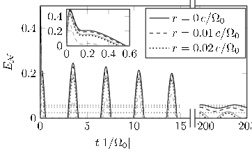
The full time evolution exhibits fast dynamics at the beginning due to the coupling of the bath being switched on suddenly, see Fig. 1. Later the entanglement oscillates until it reaches its asymptotic value. For the physically unrealistic case r=0r=0, the relative position Q2−Q1Q_{2}-Q_{1} remains undamped during the whole time evolution. The damping increases for larger distances rr. From Fig. 1 it can be deduced that the asymptotic value is reached more quickly for larger distances.
Refer to caption
Figure 1: Logarithmic negativity EE as function of time (in units of 1/Ω01/\Omega_{0}) for different distances for the 1D bath (in gray) and the 3D bath (in black). Dashed lines represent asymptotic values. The parameters are the same as in Fig. 3. A zoomed in view of the beginning of the evolution t<0.6/Ω0t<0.6/\Omega_{0} is shown in the inset.

As the maximum entanglement reached at short times is larger than the asymptotic value, one can ask the question if it features a more favorable distance dependence. We have plotted the smallest distance at which the oscillators stay separable during the entire time evolution as a function of the inverse cut-off in Fig. 2. While the distance is somewhat larger than in the asymptotic case, see Fig. 4, it can still be upper bounded by a linear function proportional to 1/Ωc1/\Omega_{c}. Therefore the qualitative behavior is the same. Exactly as in the asymptotic case, the coupling strength γ\gamma only has a minor influence on rmaxr_{\text{max}}.

Refer to caption
Figure 2: Smallest distance rmaxr_{\text{max}} at which the oscillators stay separable during the entire time evolution as a function of the inverse cut-off 1/Ωc1/\Omega_{c} for the 1D bath (in gray) and the 3D bath (in black). The parameters are the same as in Fig. 3. The inset shows rmaxr_{\text{max}} as function of the coupling strength γ\gamma.

The asymptotic state can be calculated by taking the Fourier transform of the Langevin equation (14) [19], from which we have dropped the quickly decaying term 𝐲⁡(0)​𝒞​(t)\mathbf{y}(0)\mathcal{C}(t). The resulting Quantum Langevin equation

𝐲˙​(t)+𝒵​𝐲​(t)+∫−∞td​t′​θ​(t−t′)​𝒞​(t−t′)​𝐲˙​(t′)=𝐁⁡(t)\dot{\mathbf{y}}(t)+\mathcal{Z}\mathbf{y}(t)+\int_{-\infty}^{t}dt^{\prime}\,\theta(t-t^{\prime})\mathcal{C}(t-t^{\prime})\mathbf{\dot{y}}(t^{\prime})=\mathbf{B}(t)

is transformed into the algebraic equation

−i​ω​𝐲^​(ω)+𝒵​𝐲^​(ω)−i​ω​ℛ​(ω)​𝐲^​(ω)=𝐁⁡(ω)-i\omega\hat{\mathbf{y}}(\omega)+\mathcal{Z}\hat{\mathbf{y}}(\omega)-i\omega\mathcal{R}(\omega)\hat{\mathbf{y}}(\omega)=\mathbf{B}(\omega)

with the matrix ℛ⁡(ω)\mathcal{R}(\omega) defined by

𝒞~​(ω)\displaystyle\tilde{\mathcal{C}}(\omega) =12​∫−∞∞d​t​ei​ω​t​𝒞​(t)\displaystyle=\frac{1}{2}\int_{-\infty}^{\infty}dt\,e^{i\omega t}\mathcal{C}(t)
ℛ⁡(ω)\displaystyle\mathcal{R}(\omega) =∫0∞d​t​ei​ω​t​𝒞​(t)=𝒞~​(ω)+iπ​P​∫−∞∞d​ω′​𝒞~​(ω′)ω′−ω.\displaystyle=\int_{0}^{\infty}dt\,e^{i\omega t}\mathcal{C}(t)=\tilde{\mathcal{C}}(\omega)+\frac{i}{\pi}P\int_{-\infty}^{\infty}d\omega^{\prime}\frac{\tilde{\mathcal{C}}(\omega^{\prime})}{\omega^{\prime}-\omega}\,.

The Fourier transformation of 𝒞⁡(t)\mathcal{C}(t) cancels with the integration over ω\omega, so that the matrix elements Γ~​(𝐫,ω)\tilde{\Gamma}(\mathbf{r},\omega) of 𝒞~​(ω)\tilde{\mathcal{C}}(\omega) corresponding to the elements Γ⁡(𝐫,t)\Gamma(\mathbf{r},t) of 𝒞⁡(t)\mathcal{C}(t) are simply given by

Γ~​(𝐫,ω)=π​J​(|ω|)4​|ω|​cos⁡(ω​r).\tilde{\Gamma}(\mathbf{r},\omega)=\frac{\pi J(\left|\omega\right|)}{4\left|\omega\right|}\cos(\omega r)\,.

The equilibrium equal time correlation function of the system can then be expressed in terms of the matrix

ℱ⁡(ω)=(−i​ω+𝒵−i​ω​ℛ​(ω))−1\mathcal{F}(\omega)=(-i\omega+\mathcal{Z}-i\omega\mathcal{R}(\omega))^{-1}

as the integral

⟨{𝐲i(0),𝐲j(0)}⟩=1Ω0⋅∑k,l∈{3,4}∫−∞∞d​ω​ℱi​k​(ω)​ℱj​l​(−ω)​J​(|ω|)​cos⁡(ω​r​δk​l).\langle\{\mathbf{y}_{i}(0),\mathbf{y}_{j}(0)\}\rangle=\frac{1}{\Omega_{0}}\cdot\\ \sum_{k,l\in\{3,4\}}\int_{-\infty}^{\infty}d\omega\,\mathcal{F}_{ik}(\omega)\mathcal{F}_{jl}(-\omega)J(\left|\omega\right|)\cos(\omega r\delta_{kl})\,.

The behavior of the asymptotic entanglement as a function of distance rr is plotted in Fig. 3. It drops to zero for rather small distances rmaxr_{\text{max}}, which are on the order of the inverse cut-off 1/Ωc1/\Omega_{c} as shown in Fig. 4. This is only very weakly dependent on the coupling strength, which can be explained by the fact that γ\gamma controls both coupling and decoherence at the same time. Changing it cannot be used to increase the entanglement capabilities of the bath.

Refer to caption
Figure 3: Asymptotic entanglement of the system oscillators measured in logarithmic negativity EE as a function of distance rr (in units of c/ω0c/\omega_{0}) for the 1D bath (in gray) and the 3D bath (in black), damping constant γ=Ω0\gamma=\Omega_{0}, and cut-off frequency Ωc=10​Ω0\Omega_{c}=10\Omega_{0}. EE drops to zero at a rather small critical distance rmax≲c/Ωcr_{\text{max}}\lesssim c/\Omega_{c} (cf. Fig. 4).
Refer to caption
Figure 4: Distance rmaxr_{\text{max}} at which the oscillators become asymptotically separable for the 1D bath (in gray) and the 3D bath (in black). The parameters are the same as in Fig. 3.

IV Waveguide environment

While environmentally created entanglement does not seem to be possible in free space, changing the geometry can have a big impact. A simple idea is to make the bath effectively one-dimensional by placing the two oscillators inside a waveguide with quadratic cross-section of side length aa. The quantization in transverse direction suppresses all frequencies below the first mode with frequency ω0=8​π/a\omega_{0}=\sqrt{8}\pi/a. In order to keep things simple, we will for now only consider this first mode in transverse direction. The spectrum in longitudinal direction will remain continuous.

We split the wave vector 𝐤\mathbf{k} into its components

𝐤=2​π​n1l​𝐞1+2​πa​(n2​𝐞2+n3​𝐞3).\mathbf{k}=\frac{2\pi n_{1}}{l}\mathbf{e}_{1}+\frac{2\pi}{a}(n_{2}\mathbf{e}_{2}+n_{3}\mathbf{e}_{3})\,.

with ni∈ℤ∖{0}n_{i}\in\mathbb{Z}\setminus\{0\}.

The component in 𝐞1\mathbf{e}_{1}-direction can approximated by an integral due to the large length of the tube in this direction. For this, we make a change of variables n1→|𝐤|=kn_{1}\rightarrow\left|\mathbf{k}\right|=k which implies

d​n1=l2​π​k​d​kk2−ω022​(n22+n32).\displaystyle dn_{1}=\frac{l}{2\pi}\frac{k\,dk}{\sqrt{k^{2}-\frac{\omega_{0}^{2}}{2}(n_{2}^{2}+n_{3}^{2})}}\,.

At the same time we will examine what happens to an additional term ei​𝐤𝐫e^{i\mathbf{k}\mathbf{r}} as it occurs in the damping kernel (19) and in the bath correlator (20). Assuming that 𝐫|𝐞1\mathbf{r}\parallel\mathbf{e}_{1} we find for the damping kernel

Γ⁡(𝐫,t)\displaystyle\Gamma({\mathbf{r}},t) =\displaystyle= ∫0∞d​ω​∑𝐤|g𝐤|2​δ​(ω−k)​ei​𝐤𝐫\displaystyle\int_{0}^{\infty}d\omega\sum_{\mathbf{k}}\left|g_{\mathbf{k}}\right|^{2}\delta(\omega-k)\,e^{i\mathbf{k}\mathbf{r}} (23)
=∫0∞d​ω​∑n2,n3=1ω022​(n22+n32)<ω28​l2​π​ω​|gω|2​cos⁡(ω​t)\displaystyle\hskip-56.9055pt=\int_{0}^{\infty}d\omega\sum_{n_{2},n_{3}=1}^{\frac{\omega_{0}^{2}}{2}(n_{2}^{2}+n_{3}^{2})<\omega^{2}}\frac{8l}{2\pi}\omega\left|g_{\omega}\right|^{2}\cos(\omega t)
×cos⁡(r​ω2−ω022​(n22+n32))ω2−ω022​(n22+n32)\displaystyle\hskip 28.45274pt\times\frac{\cos\left(r\sqrt{\omega^{2}-\frac{\omega_{0}^{2}}{2}(n_{2}^{2}+n_{3}^{2})}\right)}{\sqrt{\omega^{2}-\frac{\omega_{0}^{2}}{2}(n_{2}^{2}+n_{3}^{2})}}

where the factor 88 is the number of octants of a sphere. Taking in (23) the limit ω0→0\omega_{0}\rightarrow 0 and comparing with (19) we find

|gω|2=J⁡(ω)​ω024​l​ω3,\left|g_{\omega}\right|^{2}=\frac{J(\omega)\omega_{0}^{2}}{4l\omega^{3}}\,,

where we assumed isotropy of the spectral couplings, that is g𝐤=gkg_{\mathbf{k}}=g_{k}. If the oscillator frequency Ω0\Omega_{0} is close to the first excitation, we can approximate the sum in (23) by the first term n2=n3=1n_{2}=n_{3}=1. Thus, the damping kernel in the waveguide reads

Γwg​(𝐫,t)=∫0∞d​ω​Jwg​(ω)ω​cos⁡(ω​t)​cos⁡(r​ω2−ω02)\Gamma_{\mathrm{wg}}({\mathbf{r}},t)=\int_{0}^{\infty}d\omega\,\frac{J_{\mathrm{wg}}(\omega)}{\omega}\cos(\omega t)\cos\left(r\sqrt{\omega^{2}-\omega_{0}^{2}}\right)

with

Jwg(ω)=8​γ​ω02π2​ω2−ω02(ωΩc)s−1e−ω/ΩcΘ(ω−ω0).J_{\mathrm{wg}}(\omega)=\frac{8\gamma\omega_{0}^{2}}{\pi^{2}\sqrt{\omega^{2}-\omega_{0}^{2}}}\left(\frac{\omega}{\Omega_{c}}\right)^{s-1}e^{-\omega/\Omega_{c}}\Theta(\omega-\omega_{0})\,. (24)

Similarly, the bath correlator reads

Kwg​(𝐫,t)=∫0∞d​ω​Jwg​(ω)​coth⁡(ω2​T)​cos⁡(ω​t)​cos⁡(r​ω2−ω02).K_{\mathrm{wg}}({\mathbf{r}},t)=\\ \int_{0}^{\infty}d\omega\,J_{\mathrm{wg}}(\omega)\coth\left(\frac{\omega}{2T}\right)\cos(\omega t)\cos(r\sqrt{\omega^{2}-\omega_{0}^{2}})\,.

In order to approximate the full spectrum, we will use the approach depicted in Fig. 5: Only the first excitation is considered and the rest of the spectrum is replaced with the free bath. This is a good approximation as long as the oscillator frequency Ω0\Omega_{0} is close to the frequency of the first excitation ω0\omega_{0}.

Refer to caption
Figure 5: Coupling spectral density J⁡(ω)J(\omega) of a quasi one-dimensional bath. We only consider the first transversal excitation and approximate the rest of the spectrum with the free bath (black line). The full spectrum is shown in gray.

V Numerics

Due to the inverse square root divergence of the coupling spectral density, the required numerical effort is larger than in the free case. We were able to achieve good convergence by using the non-uniform distribution of grid points,

sk=smax−ω0(ngrid)2​k2+ω0\displaystyle s_{k}=\frac{s_{\mathrm{max}}-\omega_{0}}{(n_{\mathrm{grid}})^{2}}k^{2}+\omega_{0}

resulting in the kk-dependent spacing

△​sk=2​k(ngrid)2​(smax−ω0).\displaystyle\triangle s_{k}=\frac{2k}{(n_{\mathrm{grid}})^{2}}(s_{\mathrm{max}}-\omega_{0})\,.

The results of the numerical calculation are shown in the form of a density plot in Fig. 6. Shades of gray encode the value of the entanglement which is drawn as function of time (x-axis) and separation (y-axis).

Refer to caption
Figure 6: Dependence of the time evolution of the entanglement E𝒩E_{\mathcal{N}} on the spatial separation rr if the systems is placed inside of a waveguide. The value of the entanglement is encoded in the shade of gray as indicated by the scale on the right side. Additionally contour lines are drawn at the values E𝒩=0E_{\mathcal{N}}=0, 0.50.5, 11, and 1.51.5. The parameters are Ωc=10​Ω0\Omega_{c}=10\,\Omega_{0}, γ=0.05​Ω0\gamma=0.05\,\Omega_{0}, and T=0​Ω0T=0\,\Omega_{0} with an initially separable single mode squeezed state κ=10\kappa=10.
Refer to caption
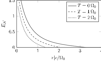
Figure 7: Distance dependence of E𝒩E_{\mathcal{N}} at t=60/Ω0t=60/\Omega_{0} for different temperatures. All other parameters are the same as in Fig. 6

We again start with a separable state, which now is a single mode squeezed state with the squeezing parameter κ=10\kappa=10

Cov⁡(0)=diag⁡(1/(κ​Ω0),1/(κ​Ω0),κ​Ω0,κ​Ω0).\operatorname{Cov}(0)=\operatorname{diag}(1/(\kappa\Omega_{0}),1/(\kappa\Omega_{0}),\kappa\Omega_{0},\kappa\Omega_{0})\,. (25)

The ground state corresponds to κ=1\kappa=1. We note that increasing the squeezing increases the absolute value of the entanglement but does not change the distance over which it is generated. The other parameters are comparable to the free case: The coupling strength is set to γ=0.05​Ω0\gamma=0.05\,\Omega_{0} and the cut-off frequency is Ωc=10​Ω0\Omega_{c}=10\,\Omega_{0}. This time, however, entanglement is generated over distances which are more than two orders of magnitude larger than in the free bath. The effect is most pronounced if the frequency of the peak ω0\omega_{0} is close to the frequency of the oscillators Ω0\Omega_{0}.

Fig. 7 shows the exact distance dependence. The plot corresponds to a vertical cut through Fig. 6 at time t=60/Ω0t=60/\Omega_{0}. Increasing the temperatures decreases the entanglement generation, but the effect persists even for comparably large temperatures of order Ω0\Omega_{0}.

VI Analytical Model

As we have seen in section (V), boundary conditions which are imposed on the bath modes have an impact on the generation of entanglement. According to equation (24), the spectral weight of the frequencies in an interval δ​ω\delta\omega centered around the van Hove peak is significantly larger than the spectral weight of frequencies in an interval δ​ω\delta\omega which is distant from the singularity. This fact can be used for a derivation of approximate analytical solutions of the model discussed in the previous section. Therefore, we take into account only the first van Hove singularity at ω0=8​π/a\omega_{0}=\sqrt{8}\pi/a and replace the coupling spectral density (24) by two effective macroscopic oscillators, representing the coherently oscillating symmetric and antisymmetric field modes around the van Hove singularity. Furthermore, we take into account for the incoherently oscillating modes of the bath by a background spectral density, given by (18). This replacement, schematically depicted in fig. 8, will be a suitable approximation as long as the modes within the van Hove peak are oscillating coherently, that is, for t,r<1/δ​ωt,r<1/\delta\omega. The effective oscillator representing the symmetric modes will determine strongly the generation of entanglement whereas dissipation and decoherence is determined by J3​DJ^{3D}.

Refer to caption
Figure 8: Schematical illustration of the replacement of the van Hove coupling spectral density by the free coupling spectral density and effective oscillators with frequency ω0\omega_{0}.

We choose 𝐫=r​𝐞1\mathbf{r}=r\mathbf{e}_{1} and decompose the system variables and the field modes in symmetric and antisymmetric compositions with respect to the 𝐞1\mathbf{e}_{1}-direction, that is

ϕ^𝐤,S/A\displaystyle\hat{\phi}_{\mathbf{k},S/A} =\displaystyle= 12​(ϕ^k1,k2,k3±ϕ^−k1,k2,k3)\displaystyle\frac{1}{\sqrt{2}}\left(\hat{\phi}_{k_{1},k_{2},k_{3}}\pm\hat{\phi}_{-k_{1},k_{2},k_{3}}\right)
Π^𝐤,S/A\displaystyle\hat{\Pi}_{\mathbf{k},S/A} =\displaystyle= 12​(Π^k1,k2,k3±Π^−k1,k2,k3)\displaystyle\frac{1}{\sqrt{2}}\left(\hat{\Pi}_{k_{1},k_{2},k_{3}}\pm\hat{\Pi}_{-k_{1},k_{2},k_{3}}\right)
Q^S/A\displaystyle\hat{Q}_{S/A} =\displaystyle= 12​(Q^1±Q^2)\displaystyle\frac{1}{\sqrt{2}}(\hat{Q}_{1}\pm\hat{Q}_{2})
P^S/A\displaystyle\hat{P}_{S/A} =\displaystyle= 12​(P^1±P^2).\displaystyle\frac{1}{\sqrt{2}}(\hat{P}_{1}\pm\hat{P}_{2})\,.

We find that the effective coupling oscillator interacts only with the symmetric mode Q^S\hat{Q}_{S}. Within this approximation, the Hamiltonian (2) reads

H^=H^B,S+H^B,A+H^0,S+H^0,A+H^int\displaystyle\hat{H}=\hat{H}_{\mathrm{B},S}+\hat{H}_{\mathrm{B},A}+\hat{H}_{0,S}+\hat{H}_{0,A}+\hat{H}_{\mathrm{int}}

with

H^B,S/A\displaystyle\hat{H}_{\mathrm{B},S/A} =\displaystyle= 12​∑k1>0,k2,k3(Π^𝐤,S​Π^−𝐤,S/A+k2​ϕ^𝐤,S​ϕ^−𝐤,S/A),\displaystyle\frac{1}{2}\sum_{k_{1}>0,k_{2},k_{3}}\left(\hat{\Pi}_{\mathbf{k},S}\hat{\Pi}_{-\mathbf{k},S/A}+k^{2}\hat{\phi}_{\mathbf{k},S}\hat{\phi}_{-\mathbf{k},S/A}\right)\,,
H^0,S\displaystyle\hat{H}_{0,S} =\displaystyle= 12​(P^S2+ΩS2​Q^S2)+12​(p^S2+ω02​q^S2)−g​p^S​Q^S,\displaystyle\frac{1}{2}\left(\hat{P}_{S}^{2}+\Omega_{S}^{2}\hat{Q}_{S}^{2}\right)+\frac{1}{2}\left(\hat{p}_{S}^{2}+\omega_{0}^{2}\hat{q}^{2}_{S}\right)-g\,\hat{p}_{S}\,\hat{Q}_{S}\,,
H^0,A\displaystyle\hat{H}_{0,A} =\displaystyle= 12​(P^A2+ΩA2​Q^A2)+12​(p^A2+ω02​q^A2),\displaystyle\frac{1}{2}\left(\hat{P}_{A}^{2}+\Omega_{A}^{2}\hat{Q}_{A}^{2}\right)+\frac{1}{2}\left(\hat{p}_{A}^{2}+\omega_{0}^{2}\hat{q}_{A}^{2}\right)\,,
H^int\displaystyle\hat{H}_{\mathrm{int}} =\displaystyle= −∑k1>0,k2,k32gk[Π^𝐤,SQ^Scos(k1​r2)\displaystyle-\sum_{k_{1}>0,k_{2},k_{3}}2g_{k}\bigg[\hat{\Pi}_{\mathbf{k},S}\hat{Q}_{S}\cos\left(\frac{k_{1}r}{2}\right)
+iΠ^𝐤,AQ^Asin(k1​r2)].\displaystyle\hskip 56.9055pt+i\hat{\Pi}_{\mathbf{k},A}\hat{Q}_{A}\sin\left(\frac{k_{1}r}{2}\right)\bigg]\,.

Here we denoted the canonical position and momentum variables of the effective oscillators with q^S/A\hat{q}_{S/A} and p^S/A\hat{p}_{S/A}, respectively. The coupling constant gg depends on the coupling spectral density and will be determined below. Furthermore, the counterterms of the Hamiltonian lead to a renormalization of the system oscillator modes, that is

ΩS/A\displaystyle\Omega_{S/A} =\displaystyle= Ω02+∫0∞d​ω​J3​D​(ω)ω​(1±sin⁡(ω​r)ω​r).\displaystyle\sqrt{\Omega_{0}^{2}+\int_{0}^{\infty}d\omega\frac{J^{3D}(\omega)}{\omega}\left(1\pm\frac{\sin(\omega r)}{\omega r}\right)}\,.

The Hamiltonian H^S\hat{H}_{\mathrm{S}} can be diagonalized by means of the transformations

ξ\displaystyle\xi =\displaystyle= ω02−ΩS2−g2+(ΩS2+g2−ω02)2+4​g2​ω022​g​ω0,\displaystyle\frac{\omega_{0}^{2}-\Omega_{S}^{2}-g^{2}+\sqrt{(\Omega_{S}^{2}+g^{2}-\omega_{0}^{2})^{2}+4g^{2}\omega_{0}^{2}}}{2g\omega_{0}}\,,
Q¯^1\displaystyle\hat{\bar{Q}}_{1} =\displaystyle= ω0​Q^S−ξ​p^ω0​1+ξ2,Q¯^2=ω0​q^−ξ​P^SΩ2​1+ξ2,\displaystyle\frac{\omega_{0}\hat{Q}_{S}-\xi\hat{p}}{\omega_{0}\sqrt{1+\xi^{2}}}\,,\quad\hat{\bar{Q}}_{2}=\frac{\omega_{0}\hat{q}-\xi\hat{P}_{S}}{\Omega_{2}\sqrt{1+\xi^{2}}}\,,
P¯^1\displaystyle\hat{\bar{P}}_{1} =\displaystyle= P^S+ξ​ω0​q^1+ξ2,P¯^2=Ω2​(p^+ξ​ω0​Q^S)ω0​1+ξ2,\displaystyle\frac{\hat{P}_{S}+\xi\omega_{0}\hat{q}}{\sqrt{1+\xi^{2}}}\,,\quad\hat{\bar{P}}_{2}=\frac{\Omega_{2}(\hat{p}+\xi\omega_{0}\hat{Q}_{S})}{\omega_{0}\sqrt{1+\xi^{2}}}\,, (26)

and adopts the canonical form

H^S\displaystyle\hat{H}_{\mathrm{S}} =\displaystyle= 12​∑i=1,2(P¯^i2+Ωi2​Q¯^i2)\displaystyle\frac{1}{2}\sum_{i=1,2}(\hat{\bar{P}}_{i}^{2}+\Omega_{i}^{2}\hat{\bar{Q}}_{i}^{2})
+\displaystyle+ OPEN12​(P¯^A2+ΩA2​Q¯^A2+p¯^A2+ω02​q¯^A2)).\displaystyle\frac{1}{2}(\hat{\bar{P}}_{A}^{2}+\Omega_{A}^{2}\hat{\bar{Q}}_{A}^{2}+\hat{\bar{p}}_{A}^{2}+\omega_{0}^{2}\hat{\bar{q}}_{A}^{2}))\,.

The eigenmodes are given by

Ω1\displaystyle\Omega_{1} =\displaystyle= 12​(ΩS2+g2+ω02+(ΩS2+g2−ω02)2+4​g2​ω02)\displaystyle\sqrt{\frac{1}{2}\left(\Omega_{S}^{2}+g^{2}+\omega_{0}^{2}+\sqrt{(\Omega_{S}^{2}+g^{2}-\omega_{0}^{2})^{2}+4g^{2}\omega_{0}^{2}}\right)}
Ω2\displaystyle\Omega_{2} =\displaystyle= 12​(ΩS2+g2+ω02−(ΩS2+g2−ω02)2+4​g2​ω02).\displaystyle\sqrt{\frac{1}{2}\left(\Omega_{S}^{2}+g^{2}+\omega_{0}^{2}-\sqrt{(\Omega_{S}^{2}+g^{2}-\omega_{0}^{2})^{2}+4g^{2}\omega_{0}^{2}}\right)}\,.

The time-evolution of the system oscillators and the coupling oscillator will be treated exactly, for the incoherently oscillating modes we will use a master equation approach.

The time evolution of the density matrix is determined by the differential equation ρ^SB=−i⁡[H^,ρ^SB]\hat{\rho}_{\mathrm{SB}}=-i[\hat{H},\hat{\rho}_{\mathrm{SB}}]. Assuming that the bath correlators decay on a time scale which is much shorter than the time scale of the system oscillators allows for a Born-Markov-approximation [2]. The density matrix of the system factorizes in a symmetric and an antisymmetric part, ρ^S=ρ^S⊗ρ^A\hat{\rho}_{\mathrm{S}}=\hat{\rho}_{S}\otimes\hat{\rho}_{A}, which obey the differential equations

∂tρ^S/A\displaystyle\partial_{t}\hat{\rho}_{S/A} =\displaystyle= −i∑i=1,2[H^S/A,ρ^S]\displaystyle-i\sum_{i=1,2}\left[\hat{H}_{S/A},\hat{\rho}_{S}\right] (27)
−∫0∞dtνS/A(t,r)[Q^S/A,[Q^S/A(−t),ρ^S/A]]\displaystyle-\int_{0}^{\infty}dt\,\nu_{S/A}(t,r)[\hat{Q}_{S/A},[\hat{Q}_{S/A}(-t),\hat{\rho}_{S/A}]]
+i∫0∞dtμS/A(t,r)[Q^S/A,{Q^S/A(−t),ρ^S/A}].\displaystyle+i\int_{0}^{\infty}dt\,\mu_{S/A}(t,r)[\hat{Q}_{S/A},\{\hat{Q}_{S/A}(-t),\hat{\rho}_{S/A}\}]\,.

The bath correlators νS/A\nu_{S/A} and μS/A\mu_{S/A} are given by

νS/A​(t,r)\displaystyle\nu_{S/A}(t,r)
=12​∫d​ω​J3​D​(ω)​coth⁡(ω2​T)​(1±sin⁡(ω​r)ω​r)​cos⁡(ω​t),\displaystyle\hskip-42.67912pt=\frac{1}{2}\int d\omega J^{3D}(\omega)\coth\left(\frac{\omega}{2T}\right)\left(1\pm\frac{\sin(\omega r)}{\omega r}\right)\cos(\omega t)\,,
μS/A​(t,r)\displaystyle\mu_{S/A}(t,r) =\displaystyle= 12​∫d​ω​J3​D​(ω)​(1±sin⁡(ω​r)ω​r)​sin⁡(ω​t).\displaystyle\frac{1}{2}\int d\omega J^{3D}(\omega)\left(1\pm\frac{\sin(\omega r)}{\omega r}\right)\sin(\omega t)\,.

Decoherence and dissipation is completely determined by the double commutators involving eight different system-bath-correlators for the symmetric and antisymmetric bath modes, respectively. The decoherence rate is determined by system-bath-correlators α1,S/A​(Ω)=∫0∞d​t​νS/A​cos⁡(Ω​t)\alpha_{1,S/A}(\Omega)=\int_{0}^{\infty}dt\,\nu_{S/A}\cos(\Omega t), the correlator α2,S/A(Ω)=−∫0∞dtνS/Asin(Ωt)/Ω\alpha_{2,S/A}(\Omega)=-\int_{0}^{\infty}dt\,\nu_{S/A}\sin(\Omega t)/\Omega is called anomalous-diffusion coefficients, α3,S/A(Ω)=−∫0∞dtμS/Acos(Ωt)\alpha_{3,S/A}(\Omega)=-\int_{0}^{\infty}dt\,\mu_{S/A}\cos(\Omega t) introduces a the lamb shift and finally α4,S/A​(Ω)=∫0∞d​t​μS/A​sin⁡(Ω​t)/Ω\alpha_{4,S/A}(\Omega)=\int_{0}^{\infty}dt\,\mu_{S/A}\sin(\Omega t)/\Omega determines the strength of dissipation. The frequency Ω\Omega is equal to Ω¯1\bar{\Omega}_{1} or Ω¯2\bar{\Omega}_{2} for the correlators with index SS and equal to ω\omega or ΩA\Omega_{A} for the correlators with index AA. Explicit expressions are given in the Appendix, see equations (38)-(41).

VI.1 Induced oscillator coupling

The effective coupling constant gg can be roughly estimated from the expressions of the correlators νS\nu_{S} or μS\mu_{S}. Splitting the wave vector as in section (IV) and replacing the n1n_{1}-summation by an integral we find

νS​(t,r)\displaystyle\nu_{S}(t,r) =\displaystyle= ∫0∞d​ω​∑n2,n3=1ω022​(n22+n32)<ω2ω02​J3​D​(ω)π​ω​ω2−ω022​(n22+n32)\displaystyle\int_{0}^{\infty}d\omega\sum_{n_{2},n_{3}=1}^{\frac{\omega_{0}^{2}}{2}(n_{2}^{2}+n_{3}^{2})<\omega^{2}}\frac{\omega_{0}^{2}J^{3D}(\omega)}{\pi\omega\sqrt{\omega^{2}-\frac{\omega_{0}^{2}}{2}(n_{2}^{2}+n_{3}^{2})}}
×coth⁡(ω2​T)​cos⁡(ω​t)​cos2⁡(r​ω2−ω022​(n12+n22)2).\displaystyle\hskip-28.45274pt\times\coth\left(\frac{\omega}{2T}\right)\cos(\omega t)\cos^{2}\left(\frac{r\sqrt{\omega^{2}-\frac{\omega_{0}^{2}}{2}(n_{1}^{2}+n_{2}^{2})}}{2}\right)\,.

Restricting ourselves to the first van Hove singularity, n2=n2=1n_{2}=n_{2}=1, and integrating from ω0\omega_{0} to ω0+δ​ω\omega_{0}+\delta\omega, we deduce the relation

g2​⟨p^​(t)​p^​ρ^B⟩\displaystyle g^{2}\langle\hat{p}(t)\hat{p}\hat{\rho}_{B}\rangle =\displaystyle= g2​ω02​cos⁡(ω0​t)​coth⁡(ω02​T)\displaystyle g^{2}\frac{\omega_{0}}{2}\cos(\omega_{0}t)\coth\left(\frac{\omega_{0}}{2T}\right)
≈\displaystyle\approx ω0π​J3​D​(ω0)​2​δ​ωω0​cos⁡(ω0​t)​coth⁡(ω02​T).\displaystyle\frac{\omega_{0}}{\pi}J^{3D}(\omega_{0})\sqrt{\frac{2\delta\omega}{\omega_{0}}}\cos(\omega_{0}t)\coth\left(\frac{\omega_{0}}{2T}\right)\,.

The modes within the van Hove peak are oscillating coherently for distances r≲c/δ​ωr\lesssim c/\delta\omega which introduces an effective distance dependence of gg. Since this coupling constant would increase indefinitely for r→0r\rightarrow 0, we need a natural cutoff for the smallest distance possible which is given by 1/Ωc1/\Omega_{c}. Therefore we have δ​ω=1/(r+1/Ωc)\delta\omega=1/(r+1/\Omega_{c}) and

g=g⁡(r)≈2​J3​D​(ω0)π​2ω0​r+ω0Ωc.\displaystyle g=g(r)\approx\sqrt{\frac{2J^{3D}(\omega_{0})}{\pi}\sqrt{\frac{2}{\omega_{0}r+\frac{\omega_{0}}{\Omega_{c}}}}}\,. (28)

VI.2 Analytical solutions

Although we restrict ourselves to Gaussian density matrices, equations (27) lead to a system of coupled nonlinear differential equations in the position representation. For this reason we transform the density matrix into the “k−Δk-\Delta”-representation [16]. Since the procedure is the same for ρ^S\hat{\rho}_{S} and ρ^A\hat{\rho}_{A}, we restrict ourselves to the former one. The transformed density matrix is given by

ρ~​(𝐤,𝚫)=Tr⁡(ρ^S​ei⁡(𝐤​𝐐¯^+𝚫​𝐏¯^)).\displaystyle\tilde{\rho}(\mathbf{k},\mathbf{\Delta})=\mathrm{Tr}\left(\hat{\rho}_{S}e^{i\left(\mathbf{k}\mathbf{\hat{\bar{Q}}}+\mathbf{\Delta}\mathbf{\hat{\bar{P}}}\right)}\right)\,.

with the vectors 𝐤=(k1,k2)T\mathbf{k}=(k_{1},k_{2})^{T}, 𝚫=(Δ1,Δ2)T\mathbf{\Delta}=(\Delta_{1},\Delta_{2})^{T}, 𝐐¯^=(Q¯^1,Q¯^2)\mathbf{\hat{\bar{Q}}}=(\hat{\bar{Q}}_{1},\hat{\bar{Q}}_{2}) and 𝐏¯^=(P¯^1,P¯^2)\mathbf{\hat{\bar{P}}}=(\hat{\bar{P}}_{1},\hat{\bar{P}}_{2}). This representation is related to the Wigner-Distribution via a double Fourier transformation and has in position representation the form

ρ~​(𝐤,𝚫)=∫d​x1​d​x2​ei​𝐤𝐱​ρS​(𝐱+𝚫2,𝐱−𝚫2)\displaystyle\tilde{\rho}(\mathbf{k},\mathbf{\Delta})=\int dx_{1}dx_{2}e^{i\mathbf{k}\mathbf{x}}\rho_{S}\left(\mathbf{x}+\frac{\mathbf{\Delta}}{2},\mathbf{x}-\frac{\mathbf{\Delta}}{2}\right)

where 𝐱=(x1,x2)\mathbf{x}=(x_{1},x_{2}) labels the diagonal elements of the density matrix. Using this particular representation we find that the master equation is linear in the derivatives with respect to kik_{i} and Δi\Delta_{i}. With an Gaussian ansatz for the density matrix ρ⁡(𝐤,𝚫)\rho(\mathbf{k},\mathbf{\Delta}) we end up with a linear first order system of differential equations, see equation (34) in the Appendix.

The dissipative part of equation (27) leads to a coupling among 14 differential equations, thus the eigenmodes cannot be found analytically. However, neglecting terms 𝒪⁡(γ​ξ)\mathcal{O}(\gamma\xi) in the dissipative part of equation (29) allows for an analytical treatment of (34). After removing the higher order couplings we are left with the usual 4 double commutators known from the Caldeira-Leggett model (see e.g.[2]).

The expectation values of the anticommutators, and therefore the negativity, can be expressed in terms of the solutions ci​(t)c_{i}(t) of the differential equations (see equations 35). From the approximate solutions (36) - (37) we find that the damping of the eigenmodes is completely determined by the dissipation-correlator. The lambshift modifies the eigenmodes Ω¯1/2\bar{\Omega}_{1/2}. We found that analytical expressions coincide very well with the numerical integration of the differential equations (34) for small and intermediate times.

Refer to caption
Figure 9: Dependence of the time evolution of the entanglement on different squeezing parameters. The remaining parameters are s=3s=3, γ=0.05​Ω0\gamma=0.05\Omega_{0}, Ωc=3​Ω0\Omega_{c}=3\Omega_{0} and r=2​[c/Ω0]r=2[c/\Omega_{0}].
Refer to caption
Figure 10: Dependence of the time evolution of the entanglement on different temperatures. The squeezing parameter is κ=5\kappa=5 and the remaining parameters are the same as in Fig. 9.

VI.3 Results

We consider the system oscillators to be initially in a Gaussian state with squeezing parameter κ\kappa, see equation (25), the effective coupling oscillator is assumed to be in the ground state. From Fig. 9 we deduce that the maximum value of the negativity depends crucially on the initial squeezing. Due to the dissipative time evolution, the system oscillators relax within intermediate times from the squeezed and nonentangled state to an entangled state with lower energy. In contrast, preparing the system initially in the ground state, that is κ=1\kappa=1, only negativity of order γ2/Ω02\gamma^{2}/\Omega_{0}^{2} is generated.

The temperature dependence is very weak for T≪Ω0T\ll\Omega_{0} whereas for T=𝒪⁡(Ω0)T=\mathcal{O}(\Omega_{0}), the negativity decreases significantly, see Fig. 10.

In virtue of the van Hove singularity we find significant entanglement over distances r≫𝒪⁡(c/Ωc)r\gg\mathcal{O}(c/\Omega_{c}) as can be deduced from Fig. 12, whereas for g=0g=0, which corresponds to the time evolution of the free space environment, we find no entanglement for distances that are larger than 𝒪⁡(c/Ωc)\mathcal{O}(c/\Omega_{c}), see Fig. 11. From the expressions (38) and (39) we see that the generation of entanglement for g=0g=0 is related to the difference between the decoherence and dissipation rates of the symmetric and antisymmetric mode, respectively.

Although various approximations were necessary in order to derive analytical expressions for the time evolution, we find good qualitative agreements with the exact numerical calculations, compare Fig. 12 with Fig. 6.

Refer to caption
Figure 11: Dependence of the time evolution of the entanglement on the spatial separation of the system oscillators without coupling oscillator. The parameters are κ=5\kappa=5, s=3s=3, γ=0.05​Ω0\gamma=0.05\Omega_{0}, Ωc=3​Ω0\Omega_{c}=3\Omega_{0} and T=0.01​[Ω0]T=0.01[\Omega_{0}].
Refer to caption
Figure 12: Dependence of the time evolution of the entanglement on the spatial separation of the system oscillators. The parameters are κ=5\kappa=5, s=3s=3, γ=0.05​Ω0\gamma=0.05\Omega_{0}, Ωc=3​Ω0\Omega_{c}=3\Omega_{0} and T=0.01​[Ω0]T=0.01[\Omega_{0}].

Taken the approximate relation (28) for granted, all entanglement vanishes in the asymptotic limit. However, treating gg and γ\gamma independently from each other we find for sufficiently large gg nonzero asymptotic negativity which can also be determined from the thermal expectation value of the covariance matrix up to corrections of order γ​ξ\mathcal{\gamma\xi}. In Fig. 13, we depict the temperature-dependence of the asymptotic entanglement for g=Ω0g=\Omega_{0} for different values of rr. From Fig. 14 we deduce that a critical minimal value of gg is necessary in order to observe asymptotically a nonzero negativity.

Refer to caption
Figure 13: Dependence of the asymptotic entanglement on the temperature for different spatial separation of the system oscillators. The parameters are s=1s=1, γ=0.01​Ω0\gamma=0.01\Omega_{0}, Ωc=3​Ω0\Omega_{c}=3\Omega_{0} and g=1​[Ω0]g=1[\Omega_{0}].
Refer to caption
Figure 14: Dependence of the asymptotic entanglement on the coupling gg for different temperatures. The parameters are s=1s~=~1, γ=0.01​Ω0\gamma=0.01\Omega_{0}, Ωc=3​Ω0\Omega_{c}=3\Omega_{0} and r=1​[c/Ω0]r~=~1[c/\Omega_{0}].

VII Conclusions

We investigated the generation of entanglement of remote quantum systems via a bosonic heat bath. Starting from an Lagrangian formulation describing the coupling of two remote harmonic oscillators to a scalar field environment, we derived the Langevin equations of motion. The coupling of the oscillators to the field momenta guaranteed the positivity of the corresponding Hamiltonian. This led to an counter-term which was already proposed in [15] in order to preserve causality and to avoid runaway solutions.

In case of a free space environment the generated entanglement drops quickly to zero if the distance between the ocsillators exceeds the spatial extension of the individual quantum systems. For one and three spatial dimensions, we found that this statement is independent of the initial conditions.

In contrary, by imposing boundary conditions on the heat bath it is possible to generate entanglement over distances which exceeds significantly the spatial extension of the quantum systems. In particular, we considered a waveguide with a transversal extension corresponding to the inverse system frequency. The boundary condition leads to a van Hove peak in the coupling spectral density. The entanglement can be enhanced significantly if the van Hove peak is in resonance with the remote quantum systems. Furthermore, the situation can be improved if the quantum systems are prepared initially in a strongly squeezed state.

Considering the coherently oscillating modes as an effective oscillator coupling the quantum systems to each other, we derived analytical solutions which are qualitatively in good agreement to the numerical results.

VIII Appendix

VIII.1 Differential equations

In order to avoid a cluttering of indices we will restrict ourselves to the density matrix for the symmetric mode and suppress the label SS. The equations determining the antisymmetric mode follow from a replacement of the eigenmodes and canonical variables in the limit ξ→0\xi\rightarrow 0. The time evolution for the oscillator variables is given by

Q¯^1/2​(t)=Q¯^1/2​cos⁡(Ω¯1/2​t)+1Ω¯1/2​P¯^1/2​sin⁡(Ω¯1/2​t),\displaystyle\hat{\bar{Q}}_{1/2}(t)=\hat{\bar{Q}}_{1/2}\cos(\bar{\Omega}_{1/2}t)+\frac{1}{\bar{\Omega}_{1/2}}\hat{\bar{P}}_{1/2}\sin(\bar{\Omega}_{1/2}t)\,,

whereas for momentum variables we find

P¯1/2​(t)=P¯1/2​cos⁡(Ω¯1/2​t)−Ω¯1/2​Q¯1/2​sin⁡(Ω¯1/2​t)\displaystyle\bar{P}_{1/2}(t)=\bar{P}_{1/2}\cos(\bar{\Omega}_{1/2}t)-\bar{\Omega}_{1/2}\bar{Q}_{1/2}\sin(\bar{\Omega}_{1/2}t)

Using relations (26) we can decompose the differential equation (27) with respect to the (time-independent) operators Q¯1/2\bar{Q}_{1/2} and P¯1/2\bar{P}_{1/2}, that is

ρ^˙\displaystyle\dot{\hat{\rho}} =\displaystyle= −i∑i=1,212[P¯^i2+Ω¯i2Q¯^i2,ρ^]\displaystyle-i\sum_{i=1,2}\frac{1}{2}\left[\hat{\bar{P}}_{i}^{2}+\bar{\Omega}_{i}^{2}\hat{\bar{Q}}_{i}^{2},\hat{\rho}\right] (29)
−α1​(Ω¯1)1+ξ2​([Q¯^1,[Q¯^1,ρ^]]+ξΩ¯2​[P¯^2,[Q¯^1,ρ^]])\displaystyle-\frac{\alpha_{1}(\bar{\Omega}_{1})}{1+\xi^{2}}\left([\hat{\bar{Q}}_{1},[\hat{\bar{Q}}_{1},\hat{\rho}]]+\frac{\xi}{\bar{\Omega}_{2}}[\hat{\bar{P}}_{2},[\hat{\bar{Q}}_{1},\hat{\rho}]]\right)
−α2​(Ω¯1)1+ξ2​([Q¯^1,[P¯^1,ρ^]]+ξΩ¯2​[P¯^2,[P¯^1,ρ^]])\displaystyle-\frac{\alpha_{2}(\bar{\Omega}_{1})}{1+\xi^{2}}\left([\hat{\bar{Q}}_{1},[\hat{\bar{P}}_{1},\hat{\rho}]]+\frac{\xi}{\bar{\Omega}_{2}}[\hat{\bar{P}}_{2},[\hat{\bar{P}}_{1},\hat{\rho}]]\right)
−ξ​α1​(Ω¯2)(1+ξ2)​Ω¯22​(ξ⁡[P¯^2,[P¯^2,ρ^]]+Ω¯2​[Q¯^1,[P¯^2,ρ^]])\displaystyle-\frac{\xi\,\alpha_{1}(\bar{\Omega}_{2})}{(1+\xi^{2})\bar{\Omega}_{2}^{2}}\bigg(\xi[\hat{\bar{P}}_{2},[\hat{\bar{P}}_{2},\hat{\rho}]]+\bar{\Omega}_{2}[\hat{\bar{Q}}_{1},[\hat{\bar{P}}_{2},\hat{\rho}]]\bigg)
+ξ​α2​(Ω¯2)1+ξ2​(ξ⁡[P¯^2,[Q¯^2,ρ^]]+Ω¯2​[Q¯^1,[Q¯^2,ρ^]])\displaystyle+\frac{\xi\,\alpha_{2}(\bar{\Omega}_{2})}{1+\xi^{2}}\bigg(\xi[\hat{\bar{P}}_{2},[\hat{\bar{Q}}_{2},\hat{\rho}]]+\bar{\Omega}_{2}[\hat{\bar{Q}}_{1},[\hat{\bar{Q}}_{2},\hat{\rho}]]\bigg)
−i​α3​(Ω¯1)1+ξ2​([Q¯^1,{Q¯^1,ρ^}]+ξΩ¯2​[P¯^2,{Q¯^1,ρ^}])\displaystyle-i\frac{\alpha_{3}(\bar{\Omega}_{1})}{1+\xi^{2}}\left([\hat{\bar{Q}}_{1},\{\hat{\bar{Q}}_{1},\hat{\rho}\}]+\frac{\xi}{\bar{\Omega}_{2}}[\hat{\bar{P}}_{2},\{\hat{\bar{Q}}_{1},\hat{\rho}\}]\right)
−i​α4​(Ω¯1)1+ξ2​([Q¯^1,{P¯^1,ρ^}]+ξΩ¯2​[P¯^2,{P¯^1,ρ^}])\displaystyle-i\frac{\alpha_{4}(\bar{\Omega}_{1})}{1+\xi^{2}}\left([\hat{\bar{Q}}_{1},\{\hat{\bar{P}}_{1},\hat{\rho}\}]+\frac{\xi}{\bar{\Omega}_{2}}[\hat{\bar{P}}_{2},\{\hat{\bar{P}}_{1},\hat{\rho}\}]\right)
−i​ξ​α3​(Ω¯2)(1+ξ2)​Ω¯22​(ξ⁡[P¯^2,{P¯^2,ρ^}]+Ω¯2​[Q¯^1,{P¯^2,ρ^}])\displaystyle-i\frac{\xi\,\alpha_{3}(\bar{\Omega}_{2})}{(1+\xi^{2})\bar{\Omega}_{2}^{2}}\bigg(\xi[\hat{\bar{P}}_{2},\{\hat{\bar{P}}_{2},\hat{\rho}\}]+\bar{\Omega}_{2}[\hat{\bar{Q}}_{1},\{\hat{\bar{P}}_{2},\hat{\rho}\}]\bigg)
+i​ξ​α4​(Ω¯2)1+ξ2​(ξ⁡[P¯^2,{Q¯^2,ρ^}]+Ω¯2​[Q¯^1,{Q¯^2,ρ^}]),\displaystyle+i\frac{\xi\,\alpha_{4}(\bar{\Omega}_{2})}{1+\xi^{2}}\bigg(\xi[\hat{\bar{P}}_{2},\{\hat{\bar{Q}}_{2},\hat{\rho}\}]+\bar{\Omega}_{2}[\hat{\bar{Q}}_{1},\{\hat{\bar{Q}}_{2},\hat{\rho}\}]\bigg)\,,

where ξ\xi was defined in equation (26) and the αi\alpha_{i} are correlation functions that are given explicitly in section VIII.3. The equations of motion in the “k−Δk-\Delta”-representation can be constructed by wrapping

Tr⁡(D^​…)=tr⁡(ei⁡(𝐤​𝐐¯^+𝚫​𝐏¯^)​…)\displaystyle\mathrm{Tr}\left(\hat{D}...\right)=\mathrm{tr}\left(e^{i\left(\mathbf{k}\mathbf{\hat{\bar{Q}}}+\mathbf{\Delta}\mathbf{\hat{\bar{P}}}\right)}...\right) (30)

over equation (32). Using the relations

Tr⁡(D^​[Q¯^i,[Q¯^j,ρ^]])\displaystyle\mathrm{Tr}(\hat{D}[\hat{\bar{Q}}_{i},[\hat{\bar{Q}}_{j},\hat{\rho}]]) =\displaystyle= Δi​Δj​ρ~\displaystyle\Delta_{i}\Delta_{j}\tilde{\rho}
Tr⁡(D^​[Q¯^i,[P¯^j,ρ^]])\displaystyle\mathrm{Tr}(\hat{D}[\hat{\bar{Q}}_{i},[\hat{\bar{P}}_{j},\hat{\rho}]]) =\displaystyle= −Δi​kj​ρ~\displaystyle-\Delta_{i}k_{j}\tilde{\rho}
Tr⁡(D^​[P¯^i,[Q¯^j,ρ^]])\displaystyle\mathrm{Tr}(\hat{D}[\hat{\bar{P}}_{i},[\hat{\bar{Q}}_{j},\hat{\rho}]]) =\displaystyle= −ki​Δj​ρ~\displaystyle-k_{i}\Delta_{j}\tilde{\rho}
Tr⁡(D^​[P¯^i,[P¯^j,ρ^]])\displaystyle\mathrm{Tr}(\hat{D}[\hat{\bar{P}}_{i},[\hat{\bar{P}}_{j},\hat{\rho}]]) =\displaystyle= ki​kj​ρ~\displaystyle k_{i}k_{j}\tilde{\rho}
Tr⁡(D^​[Q¯^i,{Q¯^j,ρ^}])\displaystyle\mathrm{Tr}(\hat{D}[\hat{\bar{Q}}_{i},\{\hat{\bar{Q}}_{j},\hat{\rho}\}]) =\displaystyle= −2iΔi∂kjρ~\displaystyle-2i\Delta_{i}\partial_{k_{j}}\tilde{\rho}
Tr⁡(D^​[Q¯^i,{P¯^j,ρ^}])\displaystyle\mathrm{Tr}(\hat{D}[\hat{\bar{Q}}_{i},\{\hat{\bar{P}}_{j},\hat{\rho}\}]) =\displaystyle= −2iΔi∂Δjρ~\displaystyle-2i\Delta_{i}\partial_{\Delta_{j}}\tilde{\rho}
Tr⁡(D^​[P¯^i,{Q¯^j,ρ^}])\displaystyle\mathrm{Tr}(\hat{D}[\hat{\bar{P}}_{i},\{\hat{\bar{Q}}_{j},\hat{\rho}\}]) =\displaystyle= 2​i​ki​∂kjρ~\displaystyle 2ik_{i}\partial_{k_{j}}\tilde{\rho}
Tr⁡(D^​[P¯^i,{P¯^j,ρ^}])\displaystyle\mathrm{Tr}(\hat{D}[\hat{\bar{P}}_{i},\{\hat{\bar{P}}_{j},\hat{\rho}\}]) =\displaystyle= 2​i​ki​∂Δjρ~,\displaystyle 2ik_{i}\partial_{\Delta_{j}}\tilde{\rho}\,, (31)

we arrive at

ρ~˙\displaystyle\dot{\tilde{\rho}} =\displaystyle= (k1−21+ξ2​α4​(Ω¯1)​(Δ1−ξΩ¯2​k2))​∂Δ1ρ~\displaystyle\left(k_{1}-\frac{2}{1+\xi^{2}}\alpha_{4}(\bar{\Omega}_{1})\left(\Delta_{1}-\frac{\xi}{\bar{\Omega}_{2}}k_{2}\right)\right)\partial_{\Delta_{1}}\tilde{\rho} (32)
+(k2−2​ξ(1+ξ2)​Ω¯22α3(Ω¯2)(Ω¯2Δ1−ξk2))∂Δ2ρ~\displaystyle+\left(k_{2}-\frac{2\xi}{(1+\xi^{2})\bar{\Omega}_{2}^{2}}\alpha_{3}(\bar{\Omega}_{2})(\bar{\Omega}_{2}\Delta_{1}-\xi k_{2})\right)\partial_{\Delta_{2}}\tilde{\rho}
−(Ω¯12Δ1+21+ξ2α3(Ω¯1)(Δ1−ξ​k2Ω¯2))∂k1ρ~\displaystyle-\left(\bar{\Omega}_{1}^{2}\Delta_{1}+\frac{2}{1+\xi^{2}}\alpha_{3}(\bar{\Omega}_{1})\left(\Delta_{1}-\frac{\xi k_{2}}{\bar{\Omega}_{2}}\right)\right)\partial_{k_{1}}\tilde{\rho}
−(Ω¯22Δ2−2​ξ1+ξ2α4(Ω¯2)(Ω¯2Δ1−ξk2))∂k2ρ~\displaystyle-\left(\bar{\Omega}_{2}^{2}\Delta_{2}-\frac{2\xi}{1+\xi^{2}}\alpha_{4}(\bar{\Omega}_{2})(\bar{\Omega}_{2}\Delta_{1}-\xi k_{2})\right)\partial_{k_{2}}\tilde{\rho}
+11+ξ2[−α1(Ω¯1)(Δ12−ξΩ¯2k2Δ1)\displaystyle+\frac{1}{1+\xi^{2}}\bigg[-\alpha_{1}(\bar{\Omega}_{1})\left(\Delta_{1}^{2}-\frac{\xi}{\bar{\Omega}_{2}}k_{2}\Delta_{1}\right)
+α2​(Ω¯1)​(k1​Δ1−ξΩ¯2​k1​k2)\displaystyle\hskip 42.67912pt+\alpha_{2}(\bar{\Omega}_{1})\left(k_{1}\Delta_{1}-\frac{\xi}{\bar{\Omega}_{2}}k_{1}k_{2}\right)
+ξΩ¯22​α1​(Ω¯2)​(Ω¯2​k2​Δ1−ξ​k22)\displaystyle\hskip 42.67912pt+\frac{\xi}{\bar{\Omega}_{2}^{2}}\alpha_{1}(\bar{\Omega}_{2})(\bar{\Omega}_{2}k_{2}\Delta_{1}-\xi\,k_{2}^{2})
+ξα2(Ω¯2)(Ω¯2Δ1Δ2−ξk2Δ2)]ρ~.\displaystyle\hskip 42.67912pt+\xi\,\alpha_{2}(\bar{\Omega}_{2})(\bar{\Omega}_{2}\Delta_{1}\Delta_{2}-\xi\,k_{2}\Delta_{2})\bigg]\tilde{\rho}\,.

With the Gaussian ansatz

ρ~QS,q\displaystyle\tilde{\rho}_{Q_{S},q} =\displaystyle= exp[−c1k12−c2k1Δ1−c3Δ12−ic4k1−ic5Δ1\displaystyle\exp\big[-c_{1}k_{1}^{2}-c_{2}k_{1}\Delta_{1}-c_{3}\Delta_{1}^{2}-ic_{4}k_{1}-ic_{5}\Delta_{1} (33)
−c6​k22−c7​k2​Δ2−c8​Δ22−i​c9​k2−i​c10​Δ2\displaystyle-c_{6}k_{2}^{2}-c_{7}k_{2}\Delta_{2}-c_{8}\Delta_{2}^{2}-ic_{9}k_{2}-ic_{10}\Delta_{2}
−c11k1k2−c12k1Δ2−c13k2Δ1−c14Δ1Δ2]\displaystyle-c_{11}k_{1}k_{2}-c_{12}k_{1}\Delta_{2}-c_{13}k_{2}\Delta_{1}-c_{14}\Delta_{1}\Delta_{2}\big]

we arrive at the first order system

c˙1\displaystyle\dot{c}_{1} =\displaystyle= c2\displaystyle c_{2}
c˙2\displaystyle\dot{c}_{2} =\displaystyle= −(2​Ω¯12+41+ξ2​α3​(Ω¯1))​c1+2​c3\displaystyle-\left(2\bar{\Omega}_{1}^{2}+\frac{4}{1+\xi^{2}}\alpha_{3}(\bar{\Omega}_{1})\right)c_{1}+2c_{3}
−11+ξ2​(2​α4​(Ω¯1)​c2−2​ξ​Ω¯2​α4​(Ω¯2)​c11CLOSE\displaystyle-\frac{1}{1+\xi^{2}}\bigg(2\alpha_{4}(\bar{\Omega}_{1})c_{2}-2\xi\bar{\Omega}_{2}\alpha_{4}(\bar{\Omega}_{2})c_{11}
OPEN+2​ξΩ¯2​α3​(Ω¯2)​c12+α2​(Ω¯1))\displaystyle+\frac{2\xi}{\bar{\Omega}_{2}}\alpha_{3}(\bar{\Omega}_{2})c_{12}+\alpha_{2}(\bar{\Omega}_{1})\bigg)
c˙3\displaystyle\dot{c}_{3} =\displaystyle= −(Ω¯12+21+ξ2​α3​(Ω¯1))​c2\displaystyle-\left(\bar{\Omega}_{1}^{2}+\frac{2}{1+\xi^{2}}\alpha_{3}(\bar{\Omega}_{1})\right)c_{2}
−11+ξ2​(4​α4​(Ω¯1)​c3−2​ξ​Ω¯2​α4​(Ω¯2)​c13CLOSE\displaystyle-\frac{1}{1+\xi^{2}}\bigg(4\alpha_{4}(\bar{\Omega}_{1})c_{3}-2\xi\bar{\Omega}_{2}\alpha_{4}(\bar{\Omega}_{2})c_{13}
OPEN+2​ξΩ¯2​α3​(Ω¯2)​c14−α1​(Ω¯1))\displaystyle+\frac{2\xi}{\bar{\Omega}_{2}}\alpha_{3}(\bar{\Omega}_{2})c_{14}-\alpha_{1}(\bar{\Omega}_{1})\bigg)
c˙4\displaystyle\dot{c}_{4} =\displaystyle= c5\displaystyle c_{5}
c˙5\displaystyle\dot{c}_{5} =\displaystyle= −(Ω¯12+21+ξ2​α3​(Ω¯1))​c4\displaystyle-\left(\bar{\Omega}_{1}^{2}+\frac{2}{1+\xi^{2}}\alpha_{3}(\bar{\Omega}_{1})\right)c_{4}
−11+ξ2​(2​α4​(Ω¯1)​c5−2​ξ​Ω¯2​α4​(Ω¯2)​c9CLOSE\displaystyle-\frac{1}{1+\xi^{2}}\bigg(2\alpha_{4}(\bar{\Omega}_{1})c_{5}-2\xi\bar{\Omega}_{2}\alpha_{4}(\bar{\Omega}_{2})c_{9}
OPEN+2​ξΩ¯2​α3​(Ω¯2)​c10)\displaystyle+\frac{2\xi}{\bar{\Omega}_{2}}\alpha_{3}(\bar{\Omega}_{2})c_{10}\bigg)
c˙6\displaystyle\dot{c}_{6} =\displaystyle= −4​ξ21+ξ2​α4​(Ω¯2)​c6+(1+2​ξ2(1+ξ2)​Ω¯22​α3​(Ω¯2))​c7\displaystyle-\frac{4\xi^{2}}{1+\xi^{2}}\alpha_{4}(\bar{\Omega}_{2})c_{6}+\left(1+\frac{2\xi^{2}}{(1+\xi^{2})\bar{\Omega}_{2}^{2}}\alpha_{3}(\bar{\Omega}_{2})\right)c_{7}
+11+ξ2​(2​ξΩ¯2​α3​(Ω¯1)​c11+2​ξΩ¯2​α4​(Ω¯1)​c13CLOSE\displaystyle+\frac{1}{1+\xi^{2}}\bigg(\frac{2\xi}{\bar{\Omega}_{2}}\alpha_{3}(\bar{\Omega}_{1})c_{11}+\frac{2\xi}{\bar{\Omega}_{2}}\alpha_{4}(\bar{\Omega}_{1})c_{13}
OPEN+ξ2Ω¯22​α1​(Ω¯2))\displaystyle+\frac{\xi^{2}}{\bar{\Omega}_{2}^{2}}\alpha_{1}(\bar{\Omega}_{2})\bigg)
c˙7\displaystyle\dot{c}_{7} =\displaystyle= −2​Ω¯22​c6−2​ξ21+ξ2​α4​(Ω¯2)​c7\displaystyle-2\bar{\Omega}_{2}^{2}c_{6}-\frac{2\xi^{2}}{1+\xi^{2}}\alpha_{4}(\bar{\Omega}_{2})c_{7}
+(2+4​ξ2(1+ξ2)​Ω¯22​α3​(Ω¯2))​c8\displaystyle+\left(2+\frac{4\xi^{2}}{(1+\xi^{2})\bar{\Omega}_{2}^{2}}\alpha_{3}(\bar{\Omega}_{2})\right)c_{8}
+11+ξ2​(2​ξΩ¯2​α3​(Ω¯1)​c12+2​ξΩ¯2​α4​(Ω¯1)​c14+ξ2​α2​(Ω¯2))\displaystyle+\frac{1}{1+\xi^{2}}\bigg(\frac{2\xi}{\bar{\Omega}_{2}}\alpha_{3}(\bar{\Omega}_{1})c_{12}+\frac{2\xi}{\bar{\Omega}_{2}}\alpha_{4}(\bar{\Omega}_{1})c_{14}+\xi^{2}\alpha_{2}(\bar{\Omega}_{2})\bigg)
c˙8\displaystyle\dot{c}_{8} =\displaystyle= −Ω¯22​c7\displaystyle-\bar{\Omega}_{2}^{2}c_{7}
c˙9\displaystyle\dot{c}_{9} =\displaystyle= c10+11+ξ2​(2​ξΩ¯2​α3​(Ω¯1)​c4+2​ξΩ¯2​α4​(Ω¯1)​c5CLOSE\displaystyle c_{10}+\frac{1}{1+\xi^{2}}\bigg(\frac{2\xi}{\bar{\Omega}_{2}}\alpha_{3}(\bar{\Omega}_{1})c_{4}+\frac{2\xi}{\bar{\Omega}_{2}}\alpha_{4}(\bar{\Omega}_{1})c_{5}
OPEN−2​ξ2​α4​(Ω¯2)​c9+2​ξ2Ω¯22​α3​(Ω¯2)​c10)\displaystyle\hskip 42.67912pt-2\xi^{2}\alpha_{4}(\bar{\Omega}_{2})c_{9}+\frac{2\xi^{2}}{\bar{\Omega}_{2}^{2}}\alpha_{3}(\bar{\Omega}_{2})c_{10}\bigg)
c˙10\displaystyle\dot{c}_{10} =\displaystyle= −Ω¯22​c9\displaystyle-\bar{\Omega}_{2}^{2}c_{9}
c˙11\displaystyle\dot{c}_{11} =\displaystyle= 11+ξ2​(4​ξΩ¯2​α3​(Ω¯1)​c1+2​ξΩ¯2​α4​(Ω¯1)​c2)\displaystyle\frac{1}{1+\xi^{2}}\left(\frac{4\xi}{\bar{\Omega}_{2}}\alpha_{3}(\bar{\Omega}_{1})c_{1}+\frac{2\xi}{\bar{\Omega}_{2}}\alpha_{4}(\bar{\Omega}_{1})c_{2}\right)
−2​ξ21+ξ2​α4​(Ω¯2)​c11+(1+2​ξ2Ω¯22​(1+ξ2))​c12\displaystyle-\frac{2\xi^{2}}{1+\xi^{2}}\alpha_{4}(\bar{\Omega}_{2})c_{11}+\left(1+\frac{2\xi^{2}}{\bar{\Omega}_{2}^{2}(1+\xi^{2})}\right)c_{12}
+c13+ξΩ¯2​(1+ξ2)​α2​(Ω¯1)\displaystyle+c_{13}+\frac{\xi}{\bar{\Omega}_{2}(1+\xi^{2})}\alpha_{2}(\bar{\Omega}_{1})
c˙12\displaystyle\dot{c}_{12} =\displaystyle= −Ω¯22​c11+c14\displaystyle-\bar{\Omega}_{2}^{2}c_{11}+c_{14}
c˙13\displaystyle\dot{c}_{13} =\displaystyle= 11+ξ2​(2​ξΩ¯2​α3​(Ω¯1)​c2+4​ξΩ¯2​α4​(Ω¯1)​c3+4​ξ​Ω¯2​α4​(Ω¯2)​c6)\displaystyle\frac{1}{1+\xi^{2}}\bigg(\frac{2\xi}{\bar{\Omega}_{2}}\alpha_{3}(\bar{\Omega}_{1})c_{2}+\frac{4\xi}{\bar{\Omega}_{2}}\alpha_{4}(\bar{\Omega}_{1})c_{3}+4\xi\bar{\Omega}_{2}\alpha_{4}(\bar{\Omega}_{2})c_{6}\bigg)
−2​ξ(1+ξ2)​Ω¯2​α3​(Ω¯2)​c7−(21+ξ2​α3​(Ω¯1)+Ω¯12)​c11\displaystyle-\frac{2\xi}{(1+\xi^{2})\bar{\Omega}_{2}}\alpha_{3}(\bar{\Omega}_{2})c_{7}-\bigg(\frac{2}{1+\xi^{2}}\alpha_{3}(\bar{\Omega}_{1})+\bar{\Omega}_{1}^{2}\bigg)c_{11}
−21+ξ2​(α4​(Ω¯1)+ξ2​α4​(Ω¯2))​c13\displaystyle-\frac{2}{1+\xi^{2}}\bigg(\alpha_{4}(\bar{\Omega}_{1})+\xi^{2}\alpha_{4}(\bar{\Omega}_{2})\bigg)c_{13}
+(1+2​ξ2(1+ξ2)​Ω¯22​α3​(Ω¯2))​c14\displaystyle+\bigg(1+\frac{2\xi^{2}}{(1+\xi^{2})\bar{\Omega}_{2}^{2}}\alpha_{3}(\bar{\Omega}_{2})\bigg)c_{14}
−ξ(1+ξ2)​Ω¯2​(α1​(Ω¯1)+α1​(Ω¯2))\displaystyle-\frac{\xi}{(1+\xi^{2})\bar{\Omega}_{2}}\bigg(\alpha_{1}(\bar{\Omega}_{1})+\alpha_{1}(\bar{\Omega}_{2})\bigg)
c˙14\displaystyle\dot{c}_{14} =\displaystyle= 11+ξ2​(2​ξ​Ω¯2​α4​(Ω¯2)​c7−4​ξΩ¯2​α3​(Ω¯2)​c8)\displaystyle\frac{1}{1+\xi^{2}}\left(2\xi\bar{\Omega}_{2}\alpha_{4}(\bar{\Omega}_{2})c_{7}-\frac{4\xi}{\bar{\Omega}_{2}}\alpha_{3}(\bar{\Omega}_{2})c_{8}\right) (34)
−(Ω¯12+21+ξ2​α3​(Ω¯1))​c12−Ω¯22​c13\displaystyle-\bigg(\bar{\Omega}_{1}^{2}+\frac{2}{1+\xi^{2}}\alpha_{3}(\bar{\Omega}_{1})\bigg)c_{12}-\bar{\Omega}_{2}^{2}c_{13}
−11+ξ2​(2​α4​(Ω¯1)​c14+ξ​Ω¯2​α2​(Ω¯2)).\displaystyle-\frac{1}{1+\xi^{2}}\left(2\alpha_{4}(\bar{\Omega}_{1})c_{14}+\xi\bar{\Omega}_{2}\alpha_{2}(\bar{\Omega}_{2})\right)\,.

The expectation values of the anticommutators can be given in terms of the functions ci​(t)c_{i}(t) according to

⟨{Q¯^1,Q¯^1}⟩\displaystyle\langle\{\hat{\bar{Q}}_{1},\hat{\bar{Q}}_{1}\}\rangle =\displaystyle= 2​(2​c1+c42)\displaystyle 2(2c_{1}+c_{4}^{2})
⟨{Q¯^1,Q¯^2}⟩\displaystyle\langle\{\hat{\bar{Q}}_{1},\hat{\bar{Q}}_{2}\}\rangle =\displaystyle= 2​(c11+c4​c9)\displaystyle 2(c_{11}+c_{4}c_{9})
⟨{Q¯^2,Q¯^2}⟩\displaystyle\langle\{\hat{\bar{Q}}_{2},\hat{\bar{Q}}_{2}\}\rangle =\displaystyle= 2​(2​c6+c92)\displaystyle 2(2c_{6}+c_{9}^{2})
⟨{Q¯^1,P¯^1}⟩\displaystyle\langle\{\hat{\bar{Q}}_{1},\hat{\bar{P}}_{1}\}\rangle =\displaystyle= 2​(c2+c4​c5)\displaystyle 2(c_{2}+c_{4}c_{5})
⟨{Q¯^2,P¯^2}⟩\displaystyle\langle\{\hat{\bar{Q}}_{2},\hat{\bar{P}}_{2}\}\rangle =\displaystyle= 2​(c7+c9​c10)\displaystyle 2(c_{7}+c_{9}c_{10})
⟨{Q¯^1,P¯^2}⟩\displaystyle\langle\{\hat{\bar{Q}}_{1},\hat{\bar{P}}_{2}\}\rangle =\displaystyle= 2​(c12+c4​c10)\displaystyle 2(c_{12}+c_{4}c_{10})
⟨{P¯^1,P¯^1}⟩\displaystyle\langle\{\hat{\bar{P}}_{1},\hat{\bar{P}}_{1}\}\rangle =\displaystyle= 2​(2​c3+c52)\displaystyle 2(2c_{3}+c_{5}^{2})
⟨{P¯^2,P¯^2}⟩\displaystyle\langle\{\hat{\bar{P}}_{2},\hat{\bar{P}}_{2}\}\rangle =\displaystyle= 2​(2​c8+c102)\displaystyle 2(2c_{8}+c_{10}^{2})
⟨{P¯^1,P¯^2}⟩\displaystyle\langle\{\hat{\bar{P}}_{1},\hat{\bar{P}}_{2}\}\rangle =\displaystyle= 2​(c14+c5​c10)\displaystyle 2(c_{14}+c_{5}c_{10})
⟨{Q¯^2,P¯^1}⟩\displaystyle\langle\{\hat{\bar{Q}}_{2},\hat{\bar{P}}_{1}\}\rangle =\displaystyle= 2​(c13+c5​c9).\displaystyle 2(c_{13}+c_{5}c_{9})\,. (35)

VIII.2 Approximate Solutions of the Differential Equations

From the initial condition (25) we find that the functions c4,c5,c9c_{4},c_{5},c_{9} and c10c_{10} are vanishing since they describe momentum and position displacements that are absent in symmetric Gaussians. At t=0t=0, the non-vanishing anticommutators have the expectation values

⟨{p^S/A,p^S/A}⟩\displaystyle\langle\{\hat{p}_{S/A},\hat{p}_{S/A}\}\rangle =\displaystyle= 1⟨{q^S/A,q^S/A}⟩=ω0\displaystyle\frac{1}{\langle\{\hat{q}_{S/A},\hat{q}_{S/A}\}\rangle}=\omega_{0}
⟨{P^S/A,P^S/A}⟩\displaystyle\langle\{\hat{P}_{S/A},\hat{P}_{S/A}\}\rangle =\displaystyle= 1⟨{Q^S/A,Q^S/A}⟩=κ​Ω0.\displaystyle\frac{1}{\langle\{\hat{Q}_{S/A},\hat{Q}_{S/A}\}\rangle}=\kappa\Omega_{0}.

Neglecting terms of order g2​γg^{2}\gamma in the differential equation, some of the equations (34) decouple from each other. For the coefficients concerning the oscillator with the variable Q¯1\bar{Q}_{1}, we find

c1\displaystyle c_{1} =\displaystyle= ∑i=13Ai​eλi​t+α1​(Ω¯1)−2​α2​(Ω¯1)​α4​(Ω¯1)4​α4​(Ω¯1)​(2​α3​(Ω¯1)+Ω¯12)\displaystyle\sum_{i=1}^{3}A_{i}e^{\lambda_{i}t}+\frac{\alpha_{1}(\bar{\Omega}_{1})-2\alpha_{2}(\bar{\Omega}_{1})\alpha_{4}(\bar{\Omega}_{1})}{4\alpha_{4}(\bar{\Omega}_{1})(2\alpha_{3}(\bar{\Omega}_{1})+\bar{\Omega}_{1}^{2})}
c2\displaystyle c_{2} =\displaystyle= ∑i=13Ai​λi​eλi​t\displaystyle\sum_{i=1}^{3}A_{i}\lambda_{i}e^{\lambda_{i}t}
c3\displaystyle c_{3} =\displaystyle= ∑i=13Ai​(λi2+Ω¯12+2​α3​(Ω¯1)+α4​(Ω¯1)​λi)​λi​eλi​t\displaystyle\sum_{i=1}^{3}A_{i}\left(\frac{\lambda_{i}}{2}+\bar{\Omega}_{1}^{2}+2\alpha_{3}(\bar{\Omega}_{1})+\alpha_{4}(\bar{\Omega}_{1})\lambda_{i}\right)\lambda_{i}e^{\lambda_{i}t} (36)
+α1​(Ω¯1)4​α4​(Ω¯1),\displaystyle+\frac{\alpha_{1}(\bar{\Omega}_{1})}{4\alpha_{4}(\bar{\Omega}_{1})}\,,

with the eigenmodes

λ1\displaystyle\lambda_{1} =\displaystyle= −2​α4​(Ω¯1)\displaystyle-2\alpha_{4}(\bar{\Omega}_{1})
λ2,3\displaystyle\lambda_{2,3} =\displaystyle= −2​(α4​(Ω¯1)±i​Ω¯12+2​α3​(Ω¯1)−α42​(Ω¯1)).\displaystyle-2\left(\alpha_{4}(\bar{\Omega}_{1})\pm i\sqrt{\bar{\Omega}_{1}^{2}+2\alpha_{3}(\bar{\Omega}_{1})-\alpha_{4}^{2}(\bar{\Omega}_{1})}\right)\,.

The AiA_{i} are chosen such that

c1​(0)\displaystyle c_{1}(0) =\displaystyle= ω0+ξ2​κ​Ω04​κ​Ω0​ω0​(1+ξ2)\displaystyle\frac{\omega_{0}+\xi^{2}\,\kappa\Omega_{0}}{4\kappa\Omega_{0}\omega_{0}(1+\xi^{2})}
c2​(0)\displaystyle c_{2}(0) =\displaystyle= 0\displaystyle 0
c3​(0)\displaystyle c_{3}(0) =\displaystyle= κ​Ω0+ξ2​ω04​(1+ξ2).\displaystyle\frac{\kappa\Omega_{0}+\xi^{2}\omega_{0}}{4(1+\xi^{2})}\,.

For the oscillator Q¯2\bar{Q}_{2} we find

c6\displaystyle c_{6} =\displaystyle= B1​e2​i​Ω¯2​t+B2​e−2​i​Ω¯2​t+B3\displaystyle B_{1}e^{2i\bar{\Omega}_{2}t}+B_{2}e^{-2i\bar{\Omega}_{2}t}+B_{3}
c7\displaystyle c_{7} =\displaystyle= 2​i​Ω¯2​B1​e2​i​Ω¯2​t−2​i​Ω¯2​B2​e−2​i​Ω¯2​t\displaystyle 2i\bar{\Omega}_{2}B_{1}e^{2i\bar{\Omega}_{2}t}-2i\bar{\Omega}_{2}B_{2}e^{-2i\bar{\Omega}_{2}t}
c8\displaystyle c_{8} =\displaystyle= −Ω¯22​(B1​e2​i​Ω¯2​t+B2​e−2​i​Ω¯2​t−B3).\displaystyle-\bar{\Omega}_{2}^{2}(B_{1}e^{2i\bar{\Omega}_{2}t}+B_{2}e^{-2i\bar{\Omega}_{2}t}-B_{3})\,.

The BiB_{i} are chosen such that

c6​(0)\displaystyle c_{6}(0) =\displaystyle= ω0+ξ2​κ​Ω04​Ω¯22​(1+ξ2)\displaystyle\frac{\omega_{0}+\xi^{2}\kappa\Omega_{0}}{4\bar{\Omega}_{2}^{2}(1+\xi^{2})}
c7​(0)\displaystyle c_{7}(0) =\displaystyle= 0\displaystyle 0
c8​(0)\displaystyle c_{8}(0) =\displaystyle= Ω¯22​(κ​Ω0+ξ2​ω0)4​κ​Ω0​ω0​(1+ξ2)\displaystyle\frac{\bar{\Omega}_{2}^{2}(\kappa\Omega_{0}+\xi^{2}\omega_{0})}{4\kappa\Omega_{0}\omega_{0}(1+\xi^{2})}

The coupling between Q¯1\bar{Q}_{1} and Q¯2\bar{Q}_{2} is described by c11​…​c14c_{11}...c_{14}, which read

c11\displaystyle c_{11} =\displaystyle= ∑i=14Ci​eκi​t\displaystyle\sum_{i=1}^{4}C_{i}e^{\kappa_{i}t} (37)
c12\displaystyle c_{12} =\displaystyle= −∑i=14Ci2​Ω¯22​(α4​(Ω¯1)+κi)2​α3​(Ω¯1)+Ω¯12−Ω¯22+2​α4​(Ω¯1)​κi+κi2eκi​t\displaystyle-\sum_{i=1}^{4}C_{i}\frac{2\bar{\Omega}_{2}^{2}(\alpha_{4}(\bar{\Omega}_{1})+\kappa_{i})}{2\alpha_{3}(\bar{\Omega}_{1})+\bar{\Omega}_{1}^{2}-\bar{\Omega}_{2}^{2}+2\alpha_{4}(\bar{\Omega}_{1})\kappa_{i}+\kappa_{i}^{2}}e^{\kappa_{i}t}
c13\displaystyle c_{13} =\displaystyle= ∑i=14Ci​κi​eκi​t\displaystyle\sum_{i=1}^{4}C_{i}\kappa_{i}e^{\kappa_{i}t}
+∑i=14Ci2​Ω¯22​(α4​(Ω¯1)+κi)2​α3​(Ω¯1)+Ω¯12−Ω¯22+2​α4​(Ω¯1)​κi+κi2eκi​t\displaystyle+\sum_{i=1}^{4}C_{i}\frac{2\bar{\Omega}_{2}^{2}(\alpha_{4}(\bar{\Omega}_{1})+\kappa_{i})}{2\alpha_{3}(\bar{\Omega}_{1})+\bar{\Omega}_{1}^{2}-\bar{\Omega}_{2}^{2}+2\alpha_{4}(\bar{\Omega}_{1})\kappa_{i}+\kappa_{i}^{2}}e^{\kappa_{i}t}
c14\displaystyle c_{14} =\displaystyle= ∑i=14Ci​Ω¯22​(2​α3​(Ω¯1)+Ω¯12−Ω¯22−κi2)2​α3​(Ω¯1)+Ω¯12−Ω¯22+2​α4​(Ω¯1)​κi+κi2​eκi​t,\displaystyle\sum_{i=1}^{4}C_{i}\frac{\bar{\Omega}_{2}^{2}(2\alpha_{3}(\bar{\Omega}_{1})+\bar{\Omega}_{1}^{2}-\bar{\Omega}_{2}^{2}-\kappa_{i}^{2})}{2\alpha_{3}(\bar{\Omega}_{1})+\bar{\Omega}_{1}^{2}-\bar{\Omega}_{2}^{2}+2\alpha_{4}(\bar{\Omega}_{1})\kappa_{i}+\kappa_{i}^{2}}e^{\kappa_{i}t}\,,

with the eigenmodes

κ1,2,3,4\displaystyle\kappa_{1,2,3,4} =\displaystyle= −α4​(Ω¯1)±i⁡(2​α3​(Ω¯1)−α42​(Ω¯1)+Ω¯12+Ω¯22CLOSE\displaystyle-\alpha_{4}(\bar{\Omega}_{1})\pm i\bigg(2\alpha_{3}(\bar{\Omega}_{1})-\alpha_{4}^{2}(\bar{\Omega}_{1})+\bar{\Omega}_{1}^{2}+\bar{\Omega}_{2}^{2}
±\displaystyle\pm OPEN2​Ω¯2​2​α3​(Ω¯1)−α42​(Ω¯1)+Ω¯12)1/2.\displaystyle 2\bar{\Omega}_{2}\sqrt{2\alpha_{3}(\bar{\Omega}_{1})-\alpha_{4}^{2}(\bar{\Omega}_{1})+\bar{\Omega}_{1}^{2}}\bigg)^{1/2}\,.

The CiC_{i} are chosen such that

c11​(0)\displaystyle c_{11}(0) =\displaystyle= 0\displaystyle 0
c12​(0)\displaystyle c_{12}(0) =\displaystyle= ξ​Ω¯2​(ω0−κ​Ω0)2​κ​Ω0​ω0​(1+ξ2)\displaystyle\frac{\xi\,\bar{\Omega}_{2}(\omega_{0}-\kappa\Omega_{0})}{2\kappa\Omega_{0}\omega_{0}(1+\xi^{2})}
c13​(0)\displaystyle c_{13}(0) =\displaystyle= ξ⁡(ω0−κ​Ω0)2​Ω¯2​(1+ξ2)\displaystyle\frac{\xi(\omega_{0}-\kappa\Omega_{0})}{2\bar{\Omega}_{2}(1+\xi^{2})}
c14​(0)\displaystyle c_{14}(0) =\displaystyle= 0.\displaystyle 0\,.

VIII.3 Bath Correlators

For the decoherence rates we find

α1,S/A​(Ω¯)=π4​J3​D​(Ω¯)​(1±sin⁡(Ω¯​r)Ω¯​r)​coth⁡(Ω¯2​T).\displaystyle\alpha_{1,S/A}(\bar{\Omega})=\frac{\pi}{4}J^{3D}(\bar{\Omega})\left(1\pm\frac{\sin(\bar{\Omega}r)}{\bar{\Omega}r}\right)\coth\left(\frac{\bar{\Omega}}{2T}\right)\,. (38)

The dissipation correlators read

α4,S/A​(Ω¯)=π​J3​D​(Ω¯)4​Ω¯​(1±sin⁡(Ω¯​r)Ω¯​r).\displaystyle\alpha_{4,S/A}(\bar{\Omega})=\frac{\pi J^{3D}(\bar{\Omega})}{4\bar{\Omega}}\left(1\pm\frac{\sin(\bar{\Omega}r)}{\bar{\Omega}r}\right)\,. (39)

The anomalous diffusion correlators have the form

α2,S/A​(Ω¯)\displaystyle\alpha_{2,S/A}(\bar{\Omega}) =\displaystyle= 2​γ​Γ​(1+s)π(Ω¯Ωc)s−1coth(Ω¯2​T)×\displaystyle\frac{2\gamma\Gamma(1+s)}{\pi}\left(\frac{\bar{\Omega}}{\Omega_{c}}\right)^{s-1}\coth\left(\frac{\bar{\Omega}}{2T}\right)\times (40)
×[e−Ω¯Ωc(cos(πs)ℜ{Γ(−s,−Ω¯Ωc)}\displaystyle\hskip-56.9055pt\times\Bigg[e^{-\frac{\bar{\Omega}}{\Omega_{c}}}\bigg(\cos(\pi s)\Re\left\{\Gamma\left(-s,-\frac{\bar{\Omega}}{\Omega_{c}}\right)\right\}
−sin(πs)ℑ{Γ(−s,−Ω¯Ωc)})+eΩ¯ΩcΓ(−s,Ω¯Ωc)]\displaystyle\hskip-56.9055pt-\sin(\pi s)\Im\left\{\Gamma\left(-s,-\frac{\bar{\Omega}}{\Omega_{c}}\right)\right\}\bigg)+e^{\frac{\bar{\Omega}}{\Omega_{c}}}\Gamma\left(-s,\frac{\bar{\Omega}}{\Omega_{c}}\right)\Bigg]
−8​T​γ​Ωc​Γ​(1+s)π​(1Ω¯2​s+∑n=1∞(2​π​n​TΩc)s​cnΩ¯2+(2​π​n​T)2)\displaystyle\hskip-56.9055pt-\frac{8T\gamma\Omega_{c}\Gamma(1+s)}{\pi}\left(\frac{1}{\bar{\Omega}^{2}s}+\sum_{n=1}^{\infty}\left(\frac{2\pi nT}{\Omega_{c}}\right)^{s}\frac{c_{n}}{\bar{\Omega}^{2}+(2\pi nT)^{2}}\right)
±{−γ​Γ​(s−1)π​r​Ωc(Ω¯Ωc)s−2coth(Ω¯2​T)×\displaystyle\hskip-56.9055pt\pm\Bigg\{-\frac{\gamma\Gamma(s-1)}{\pi r\Omega_{c}}\left(\frac{\bar{\Omega}}{\Omega_{c}}\right)^{s-2}\coth\left(\frac{\bar{\Omega}}{2T}\right)\times
×[2cos(Ω¯r)e−Ω¯Ωc(sin(πs)ℜ{Γ(−s+2,−Ω¯Ωc)}\displaystyle\hskip-56.9055pt\times\Bigg[2\cos(\bar{\Omega}r)e^{-\frac{\bar{\Omega}}{\Omega_{c}}}\bigg(\sin(\pi s)\Re\left\{\Gamma\left(-s+2,-\frac{\bar{\Omega}}{\Omega_{c}}\right)\right\}
OPEN+cos⁡(π​s)​ℑ⁡{Γ⁡(−s+2,−Ω¯Ωc)})\displaystyle\hskip-56.9055pt+\cos(\pi s)\Im\left\{\Gamma\left(-s+2,-\frac{\bar{\Omega}}{\Omega_{c}}\right)\right\}\bigg)
+i​eΩ¯​(1Ωc+i​r)​Γ​(−s+2,Ω¯​(1Ωc+i​r))\displaystyle\hskip-56.9055pt+ie^{\bar{\Omega}\left(\frac{1}{\Omega_{c}}+ir\right)}\Gamma\left(-s+2,\bar{\Omega}\left(\frac{1}{\Omega_{c}}+ir\right)\right)
−i​eΩ¯​(1Ωc−i​r)​Γ​(−s+2,Ω¯​(1Ωc−i​r))\displaystyle\hskip-56.9055pt-ie^{\bar{\Omega}\left(\frac{1}{\Omega_{c}}-ir\right)}\Gamma\left(-s+2,\bar{\Omega}\left(\frac{1}{\Omega_{c}}-ir\right)\right)
−i​e−Ω¯​(1Ωc+i​r)−i​π​s​Γ​(−s+2,−Ω¯​(1Ωc+i​r))\displaystyle\hskip-56.9055pt-ie^{-\bar{\Omega}\left(\frac{1}{\Omega_{c}}+ir\right)-i\pi s}\Gamma\left(-s+2,-\bar{\Omega}\left(\frac{1}{\Omega_{c}}+ir\right)\right)
+ie−Ω¯​(1Ωc−i​r)+i​π​sΓ(−s+2,−Ω¯(1Ωc−ir))]\displaystyle\hskip-56.9055pt+ie^{-\bar{\Omega}\left(\frac{1}{\Omega_{c}}-ir\right)+i\pi s}\Gamma\left(-s+2,-\bar{\Omega}\left(\frac{1}{\Omega_{c}}-ir\right)\right)\Bigg]
+4​γ​T​Γ​(s−1)π​r∑n=1∞(2​π​n​TΩc)s−1dnΩ¯2+(2​π​n​T)2}\displaystyle\hskip-56.9055pt+\frac{4\gamma T\Gamma(s-1)}{\pi r}\sum_{n=1}^{\infty}\left(\frac{2\pi nT}{\Omega_{c}}\right)^{s-1}\frac{d_{n}}{\bar{\Omega}^{2}+(2\pi nT)^{2}}\Bigg\}

with

cn\displaystyle c_{n} =\displaystyle= e−i​2​π​n​TΩc−i​π​s2​Γ​(−s,−i​2​π​n​TΩc)\displaystyle e^{-i\frac{2\pi nT}{\Omega_{c}}-i\frac{\pi s}{2}}\Gamma\left(-s,-i\frac{2\pi nT}{\Omega_{c}}\right)
+\displaystyle+ ei​2​π​n​TΩc+i​π​s2​Γ​(−s,i​2​π​n​TΩc);\displaystyle e^{i\frac{2\pi nT}{\Omega_{c}}+i\frac{\pi s}{2}}\Gamma\left(-s,i\frac{2\pi nT}{\Omega_{c}}\right)\,;
dn\displaystyle d_{n} =\displaystyle= ei​2​π​n​T​(1Ωc+i​r)+i​π​s2​Γ​(−s+2,i​2​π​n​T​(1Ωc+i​r))\displaystyle e^{i2\pi nT\left(\frac{1}{\Omega_{c}}+ir\right)+i\frac{\pi s}{2}}\Gamma\left(-s+2,i2\pi nT\left(\frac{1}{\Omega_{c}}+ir\right)\right)
+\displaystyle+ e−i​2​π​n​T​(1Ωc−i​r)−i​π​s2​Γ​(−s+2,−i​2​π​n​T​(1Ωc−i​r))\displaystyle e^{-i2\pi nT\left(\frac{1}{\Omega_{c}}-ir\right)-i\frac{\pi s}{2}}\Gamma\left(-s+2,-i2\pi nT\left(\frac{1}{\Omega_{c}}-ir\right)\right)
−\displaystyle- e−i​2​π​n​T​(1Ωc+i​r)−i​π​s2​Γ​(−s+2,−i​2​π​n​T​(1Ωc+i​r))\displaystyle e^{-i2\pi nT\left(\frac{1}{\Omega_{c}}+ir\right)-i\frac{\pi s}{2}}\Gamma\left(-s+2,-i2\pi nT\left(\frac{1}{\Omega_{c}}+ir\right)\right)
+\displaystyle+ ei​2​π​n​T​(1Ωc−i​r)+i​π​s2​Γ​(−s+2,i​2​π​n​T​(1Ωc−i​r)).\displaystyle e^{i2\pi nT\left(\frac{1}{\Omega_{c}}-ir\right)+i\frac{\pi s}{2}}\Gamma\left(-s+2,i2\pi nT\left(\frac{1}{\Omega_{c}}-ir\right)\right)\,.

The Lamb shifts due to the bath correlators are given by

α3,S/A​(Ω¯)\displaystyle\alpha_{3,S/A}(\bar{\Omega}) =\displaystyle= −2​γ​Γ​(3+s)​Ω¯π(Ω¯Ωc)s−1×\displaystyle-\frac{2\gamma\Gamma(3+s)\bar{\Omega}}{\pi}\left(\frac{\bar{\Omega}}{\Omega_{c}}\right)^{s-1}\times (41)
×[e−Ω¯Ωc(cos(πs)ℜ{Γ(−2−s,−Ω¯Ωc)}\displaystyle\hskip-56.9055pt\times\Bigg[e^{-\frac{\bar{\Omega}}{\Omega_{c}}}\bigg(\cos(\pi s)\Re\left\{\Gamma\left(-2-s,-\frac{\bar{\Omega}}{\Omega_{c}}\right)\right\}
OPEN−sin⁡(π​s)​ℑ⁡{Γ⁡(−2−s,−Ω¯Ωc)})\displaystyle\hskip-56.9055pt-\sin(\pi s)\Im\left\{\Gamma\left(-2-s,-\frac{\bar{\Omega}}{\Omega_{c}}\right)\right\}\bigg)
+eΩ¯ΩcΓ(−2−s,Ω¯Ωc)]+4​γ​Ωc3​Γ​(3+s)π​Ω¯2​(2+s)\displaystyle\hskip-56.9055pt+e^{\frac{\bar{\Omega}}{\Omega_{c}}}\Gamma\left(-2-s,\frac{\bar{\Omega}}{\Omega_{c}}\right)\Bigg]+\frac{4\gamma\Omega_{c}^{3}\Gamma(3+s)}{\pi\bar{\Omega}^{2}(2+s)}
±{γ​Γ​(1+s)π​r(Ω¯Ωc)s−1×\displaystyle\hskip-56.9055pt\pm\Bigg\{\frac{\gamma\Gamma(1+s)}{\pi r}\left(\frac{\bar{\Omega}}{\Omega_{c}}\right)^{s-1}\times
×[2cos(Ω¯r)e−Ω¯Ωc(sin(πs)ℜ{Γ(−s,−Ω¯Ωc)}\displaystyle\hskip-56.9055pt\times\Bigg[2\cos(\bar{\Omega}r)e^{-\frac{\bar{\Omega}}{\Omega_{c}}}\bigg(\sin(\pi s)\Re\left\{\Gamma\left(-s,-\frac{\bar{\Omega}}{\Omega_{c}}\right)\right\}
OPEN+cos⁡(π​s)​ℑ⁡{Γ⁡(−s,−Ω¯Ωc)})\displaystyle\hskip-56.9055pt+\cos(\pi s)\Im\left\{\Gamma\left(-s,-\frac{\bar{\Omega}}{\Omega_{c}}\right)\right\}\bigg)
+i​eΩ¯​(1Ωc+i​r)​Γ​(−s,Ω¯​(1Ωc+i​r))\displaystyle\hskip-56.9055pt+ie^{\bar{\Omega}\left(\frac{1}{\Omega_{c}}+ir\right)}\Gamma\left(-s,\bar{\Omega}\left(\frac{1}{\Omega_{c}}+ir\right)\right)
−i​eΩ¯​(1Ωc−i​r)​Γ​(−s,Ω¯​(1Ωc−i​r))\displaystyle\hskip-56.9055pt-ie^{\bar{\Omega}\left(\frac{1}{\Omega_{c}}-ir\right)}\Gamma\left(-s,\bar{\Omega}\left(\frac{1}{\Omega_{c}}-ir\right)\right)
−i​e−Ω¯​(1Ωc+i​r)−i​π​s​Γ​(−s,−Ω¯​(1Ωc+i​r))\displaystyle\hskip-56.9055pt-ie^{-\bar{\Omega}\left(\frac{1}{\Omega_{c}}+ir\right)-i\pi s}\Gamma\left(-s,-\bar{\Omega}\left(\frac{1}{\Omega_{c}}+ir\right)\right)
+ie−Ω¯​(1Ωc−i​r)+i​π​sΓ(−s,−Ω¯(1Ωc−ir))]}.\displaystyle\hskip-56.9055pt+ie^{-\bar{\Omega}\left(\frac{1}{\Omega_{c}}-ir\right)+i\pi s}\Gamma\left(-s,-\bar{\Omega}\left(\frac{1}{\Omega_{c}}-ir\right)\right)\Bigg]\Bigg\}\,.

The Lamb shifts originating from the counter terms are determined by

∫0∞d​ω​J3​D​(ω)ω​(1±sin⁡(ω​r)ω​r)=8​γ​Ωcπ​(Γ⁡(s)CLOSE\displaystyle\int_{0}^{\infty}d\omega\frac{J^{3D}(\omega)}{\omega}\left(1\pm\frac{\sin(\omega r)}{\omega r}\right)=\frac{8\gamma\Omega_{c}}{\pi}\bigg(\Gamma(s) (42)
OPEN±(1+Ωc2​r2)−s−12​Γ​(s−1)​sin⁡[(s−1)​arctan⁡(Ωc​r)]Ωc​r).\displaystyle\pm\frac{(1+\Omega_{c}^{2}r^{2})^{-\frac{s-1}{2}}\Gamma(s-1)\sin\left[(s-1)\arctan(\Omega_{c}r)\right]}{\Omega_{c}r}\bigg)\,.

References

  • [1] E. Joos et al., Decoherence and the Appearance of a Classical World in Quantum Theory, Springer (2003).
  • [2] M. Schlosshauer, Decoherence and the Quantum-to-Classical Transition, Springer (2007).
  • [3] D. Braun, Phys. Rev. Lett. 89, 277901 (2002).
  • [4] F. Benatti, R. Floreanini and M. Piani, Phys. Rev. Lett. 91, 070402 (2003).
  • [5] D. Braun, Daniel, Phys. Rev. A 72, 062324 (2005).
  • [6] F. Benatti and R. Floreanini, J. Phys. A 39, 2689 (2006).
  • [7] S. Oh and J. Kim, Phys. Rev. A 73, 062306 (2006).
  • [8] J. S. Prauzner-Bechcicki, J. Phys. A, 37, L173 (2004).
  • [9] J. H. An and W. M. Zhang, Phys. Rev. A 76, 042127 (2007).
  • [10] C.-H. Chou, T. Yu and B. L. Hu, Phys. Rev. E 77, 011112 (2008).
  • [11] K.-L. Liu and H.-S. Goan, Phys. Rev. A 76, 022312 (2007).
  • [12] C. Hörhammer and H. Büttner, Phys. Rev. A 77, 042305 (2008).
  • [13] J. P. Paz and A. J. Roncaglia, Phys. Rev. Lett. 100, 220401 (2008).
  • [14] D. Solenov, D. Tolkunov and V. Privman, Phys. Rev. B 75, 035134 (2007).
  • [15] T. Zell, F. Queisser and R. Klesse, Phys. Rev. Lett. 102, 160501 (2009).
  • [16] W. G. Unruh and W. H. Zurek, Phys. Rev. D, 40, 1071 (1989).
  • [17] J. Wilkie and Y. M. Wong, J. Phys. A 41, 335005 (2008).
  • [18] G. Vidal and R. F. Werner, Phys. Rev. A 65, 032314 (2002).
  • [19] C. W. Gardiner and P. Zoller, Quantum Noise, Springer (2004).