A graph theoretical Gauss-Bonnet-Chern Theorem
Abstract.
We prove a discrete Gauss-Bonnet-Chern theorem for finite graphs , where is the vertex set and is the edge set of the graph. The dimension of the graph, the local curvature form and the Euler characteristic are all defined graph theoretically.
Key words and phrases:
Graph theory, Gauss-Bonnet, Curvature1991 Mathematics Subject Classification
Primary: 05C10 , 57M151. Introduction
The Gauss-Bonnet-Chern theorem for a compact
-dimensional Riemannian manifold generalizes the Gauss-Bonnet
theorem for compact -dimensional surfaces. It averages the Euler curvature form
, the Pfaffian of the curvature form
over the manifold, and leads to the Euler characteristic .
First tackled by Allendoerfer and Fenchel for surfaces
in Euclidean space and extended by
Allendoerfer and Weil to closed Riemannian manifolds,
it was Chern, whose 100’th birthday we celebrate this year,
who first gave an intrinsic proof [1].
Modern proofs use Fermionic calculus [18, 6] which becomes
especially elegant in Patodi’s approach [6].
We introduce here an Euler curvature form for graphs
which only depends on the number of -dimensional pieces of the unit sphere
at with . Since by definition, we have a -dimensional
graph , the unit sphere at a point is a -dimensional graph.
While Puiseux type formulas allow to discretize curvature in two dimensions,
the lack of a natural second order difference calculus for graphs prevents a
straightforward translation of the classical Euler curvature form to graph theory so that we construct
it from scratch using some assumptions on graphs so that everything stays elementary.
For four dimensional graphs for example, the curvature form at depends only on the
number of edges and faces of the three dimensional sphere centered at .
For two-dimensional graphs, the Euler curvature form is ,
where is the arc length of the unit circle .
This curvature traces back to a combinatorial curvature defined in [9], where differential geometry is
pushed to more general spaces. Gromov’s graph theoretical curvature is up to a normalization defined by
, where are the cardinalities of the neighboring face degrees
for vertices in the sphere . For two dimensional graphs, where necessarily all faces are triangles,
this simplifies to so that , where is the cardinality of the sphere of radius 1.
If is a cyclic graph, then the arc length and vertex cardinality of the sphere are the same.
The combinatorial curvature illustrates the -condition for non-positive curvature and
that leads to strictly negative curvature.
For two-dimensional graph with or without boundary, the result
appears in [14], where was scaled to avoid fractions.
We do not rescale the discrete Euler form in this article because with increasing dimensions, the denominator terms
become larger and would have to be scaled in a dimension-dependent manner to be rendered integer valued. We could
work with which is an integer but leave the fractions.
For two dimensional graphs, the sphere of a vertex is one-dimensional graph
without boundary, a cyclic graph. In three dimensions, the Euler curvature form
vanishes identically. For four-dimensional graphs, which is already a new case, the curvature form
is , where is the number of edges of the unit sphere and where is
the number of faces in .
For 5 dimensional graphs, the curvature form is . It would be zero if .
We do not know yet whether it is always identically zero, even so the sum over the entire graph is.
Also the examples of 5-dimensional graphs we looked at, .

The core mechanism for relating global Euler characteristic and local curvature for general finite undirected graphs is the following: the total number of dimensional simplices in is related to the number of dimensional simplices in the unit sphere by . Then with curvature
| (1) |
where we use that .
We have just seen a very general Gauss-Bonnet theorem relating a local curvature form with a global quantity:
For any finite graph without self-loops and multiple connections, we have , where is a curvature form defined in Equation (1) which depends only on the unit sphere of a vertex .
Here are some examples. For a discrete graph with vertices without edges,
the unit spheres are all empty and sums up to .
For the complete graph , we have and
since is we have adding up to .
For a tree, the curvature of a vertex is .
The sum of the curvatures of a single tree is and the total curvature of a forest the number of trees.
For a wheel graph with vertices and edges and faces, we have . The
central vertex has , the other points
have . The total curvature is .
For an octahedron , we have and and
since each unit sphere is the circular graph so that
the total curvature is .
For a cube with we get reflecting the fact that we have holes.
Because consists of discrete points, we have
everywhere and the sum is . If we stellate the cube, it becomes
dimensional and the data lead to .
The original vertices have zero curvature , the six new ones
satisfy and the total curvature is .
As we have just seen, Gauss-Bonnet-Chern is elementary and works for general graphs. Despite that it can be stated and proven quickly, the topic is far from trivial. We explore it here in a setting close to differential geometry, where all unit spheres have properties known to spheres in . While the topic is accessible to high school mathematics, there are many open questions. For example, we do not yet have cases of 5 dimensional graphs, where the Euler curvature form is not identically zero which makes us believe that it is always zero in odd dimensions. Concrete examples can become tedious to compute by hand in higher dimensions and computers are essential for exploration. A triangularization of the dimensional cube for example which can be realized as a convex polytope in leads to a graph with 536 vertices and 8216 edges which has five different types of dimensional unit spheres. Still, the curvature form for is identically zero at every point. Also combinatorial problems appear. Discrete versions of Bonnet-Schoenberg-Myers bounds show that there are only finitely many dimensional graphs where all sectional curvatures are strictly positive meaning that every two dimensional subgraph has strictly positive curvature. Up to isomorphisms, there are six for . How many are there in ? Also Ricci curvature , a function on the edge set which gives the sum over all curvatures of dimensional wheel graphs containing a given edge is unexplored. Any question in differential topology can be considered for -dimensional graphs. For example, Chern proved that for four dimensional manifolds with nonpositive sectional curvatures, the Euler curvature form is nonnegative. Is it true that for a dimensional graph the curvature form is nonnegative if every two dimensional wheel subgraph of has or more spikes?
2. The theorem
Throughout the paper we work in a graph theoretical setup. We especially do not
assume anywhere that graphs are embedded in any ambient Euclidean space, nor assume the graph to be a
triangularization of a smooth manifold. All graphs are finite undirected graphs
without self loops and without multiple edges. Any conceptual discretization of differential
geometry to graph theory requires to give a graph theoretical definition of what
dimension means for a graph. We work with the inductive graph dimension given
in [14] but make an additional assumption about the topology of the unit sphere.
The later is essential to be close to geometry. It even narrows the class of dimensional
graphs because as we will see, there are -dimensional graphs in which unit spheres can
have any prescribed Euler characteristic possible in the continuum.
Let denote the number of -dimensional subgraphs of a graph which are simplices, complete graphs with vertices. The Euler characteristic of a -dimensional graph is defined as
For dimensions for example, we have , , the number of vertices, edges and faces and .
Definition 1.
A graph with vertices and edges is called a -dimensional graph without boundary if at every vertex , the unit sphere is a connected -dimensional graph without boundary of Euler characteristic . This is an inductive definition which also should apply to unit spheres. We additionally make the assumption that . Together with the assumption that a graph without any edges is zero-dimensional, this defines dimension inductively.
By adding to the average of the dimensions of all spheres, we can define inductively dimension for all graphs, but the dimension becomes fractional in general. Figure () for example displays a fantasy graph of dimension .
3. The Euler Curvature form
Define the fractions ,
and the integers . The later is for even and for odd .
Here are the first entries:
| n | 1 | 2 | 3 | 4 | 5 | 6 | 7 | … |
|---|---|---|---|---|---|---|---|---|
| -1/6 | 1/4 | -3/10 | 1/3 | -5/14 | 3/8 | -7/18 | … | |
| 0 | 1 | 0 | 1 | 0 | 1 | 0 | … |
Definition 2.
The Euler curvature form at a vertex in a -dimensional graph is defined as if and
for .
Remark 1. The curvature form depends on the sphere quantities
if and on only one sphere quantity if .
Remark 2. If we would not use the hyper relations, we could work with the more elegant and symmetric
curvature . Without Euler characteristic assumption, we could even
use the curvature Equation (1) given in the introduction. While less
geometric, it has the elegance of the Euler curvature in the continuum, if we define so that
written as .
Remark 3. How can equation (1) be related to the Euler curvature form
used in the classical Gauss-Bonnet-Chern? Here is as close as we could get:
with a “super operator” satisfying for we have
. If were skew symmetric then this is
with Pfaffian and would also establish in odd dimensions.
Discrete curvature when summed up is formally close to a ”height” construction
in differential geometry, where is the Laplacian with a zeta regularized determinant.
Rewriting Gauss-Bonnet-Chern as is a naive discrete analogue of
the McKean-Singer formula because solving is replaced by
solving the discrete heat flow . While this is only formal,
it adds hope that is zero in odd dimensions and differential geometric assumptions done here.
For the following low-dimensional cases, we use the notation :
| dim | Euler form | simplified |
|---|---|---|
| d=2 | 1-E/6 | 1-E/6 |
| d=3 | -E/6+(2/3) E/4 | 0 |
| d=4 | 1-E/6+F/4-(2/4) 3F/10 | 1 -E/6 + F/10 |
| d=5 | -E/6+F/4-3C/10 +(2/5)C/3 | -E/6 + F/4 - C/6 |
| d=6 | 1-E/6+F/4-3C/10+S/3-(2/6)5S/14 | 1-E/6+F/4-3C/10+3S/14 |
| d=7 | -E/6+F/4-3C/10+S/3-(5H/14)+(2/7)3H/8 | -E/6+F/4-3C/10+S/3-H/4 |
Our main result is that integrating the Euler curvature form over the graph is equal to the Euler characteristic:
Theorem 1 (Discrete Gauss-Bonnet-Chern).
If is a finite -dimensional graph, then
Remark 1. Theorem 1 reduces to Gauss-Bonnet for two dimensional graphs
discussed in the second part of [14].
As stressed in that article, all notions which enter the theorem are purely graph theoretical and no additional
structure is required. In the same way that objects in differential topology are of
primary interest, if they are defined intrinsically and in a coordinate independent way,
we do not want to refer to an ambient structure or assume
non graph theoretically defined notions. A large field of discrete differential geometry
does include more information like angles or distances to be able to approximate given smooth structures.
Discrete differential geometry has grown in many flavors: Regge calculus [5] is used
in general relativity, digital topology in computer vision, simplicial cohomology for algebraic topology,
or computational geometry in numerical methods of computer graphics [7].
Graph theoretical approaches not using any other structures appear in network theory [3].
Remark 2. The inductive dimension for graphs [14]
is closely related to the inductive Brower-Menger-Urysohn dimension for topological spaces
which goes back to the later work of
Poincaré [12, 8, 17]. This dimension is the smallest such that every point has arbitrary small neighborhoods
such that the boundary of has inductive dimension and the
empty set has dimension [12].
For a normal topological space with countable base, the inductive dimension is equal to
the topological dimension by Urysohn’s metrization theorem.
It is different from the inductive graph dimension defined in [14] because both
”topological inductive dimension” and ”covering dimension” are zero for finite graphs where the discrete topology of
all subsets it the only natural topology. There are other notions of ”dimension”:
the ”topological dimension” of a graph always (e.g. [16] page 305),
the ”metric dimension” is the minimum number of vertices of a subset of
such that every is uniquely defined by the distances to points in . The
”fractal dimension” for infinite graphs measures the growth rate [3].
Also these are obviously different dimensions.
Remark 3. The curvature form defined here is local in the sense that it only depends on the
geometry of the unit ball centered at the vertex . Theorem 1 is interesting because it links
deformable local properties with rigid global topological properties.
Remark 4. The discrete Gauss-Bonnet-Chern result is not a discrete approximation of the classical
Gauss-Bonnet-Chern theorem because curvature takes a prescribed discrete set of values and can not
become arbitrarily fine. Triangularizations allow to approximate -dimensional
manifolds by d-dimensional graphs but already the case of the two dimensional sphere,
illustrated by geodesic domes, golf or buckyballs, shows that curvature is located on 12 points only,
independent how fine the grid is. This implies for large graphs that most of the graph is flat.
In spirit the continuum and discrete results are the same result: the curvature is a local property which depends on the metric
the Euler characteristic is global and a topological quantity. They are related in a global manner.
Remark 5. The previous remark does not exclude less naive connections between the discrete and continuum.
Here is one: we could relate the continuous Gauss-Bonnet-Chern theorem with the discrete version by taking random
triangularizations for which the expectation value of the discrete curvature is the classical curvature.
Remark 6. The discrete curvature form changes during ”homotopy deformations” of the graph but
the Euler characteristic does not. The discrete version of Euler form might be more accessible to geometric
interpretations since (to cite[15]) ”The only problem with the Gauss-Bonnet-Chern
result is that the relationship between the Pfaffian and sectional curvatures is obscure in higher
dimensions, so no one seems to have any idea how to interpret the theorem geometrically!”
As in classical differential geometry, the geometry of spheres near a point
determines the Euler curvature form. In classical differential geometry, the curvature tensor is
accessible through sectional curvatures which can be measured using Bertrand-Puiseux formulas from lengths
of circles on two dimensional geodesic sheets.
There are Puisaux curvature formulas which do not refer to an underlying flat
situation like , where is the length of the sphere
of radius in the sheet where is a two dimensional plane in the tangent
space . The classical curvature form of a manifold is
determined from the lengths of circles of radius and in a circle
obtained by intersecting the sphere with the plane spanned by and .
Remark 7. Even so the following quote of [2] appeared in the context of
spectral graph theory, it hits the heart of matter:
”Although differential geometry and spectral graph theory share a great deal
in common, there is no question that significant differences exist. Obviously a graph is not ”differentiable”
and many geometrical techniques involving high-order
derivatives could be very difficult, if not impossible to utilize for graphs. There are substantial
obstacles for deriving the discrete analogues of many of the known results in the continuous case.
Nevertheless, there are many successful examples developing the discrete parallels, and
this process sometimes leads to improvement and strengthening of the original results from the continuous case.”
If there is a discrete Gauss-Bonnet-Chern theorem with second order notions, then this would be closer to the
continuum, but this is more subtle and applies only to a much more restricted set of graphs.
Even for the two dimensional Gauss-Bonnet theorem, there are challenges to identify the set
of graphs in which second order curvatures like work.
Remark 8. The study of dimension of graphs is also interesting in random graph theory. We have explicit formulas for the average dimension of a graph with vertices where each edge is
switched on with probability . But the statistics of dimension is largely unexplored. We see experimentally
for example that both in random and concrete networks, points with integer dimension have higher probability.
Remark 9. Since [14] was written, we also found out more about the origin of combinatorial curvature:
Higuchi [11] uses a definition of an unpublished talk by Ishida from 1990, the
combinatorial curvature
which is dual to a curvature defined by Gromov [9] in 1987. Higuchi
poses a question whether the positivity of
for a planar graph in which is a closed circuit everywhere implies that the graph is finite.
He also mentions . This is in our notation,
for two-dimensional graphs, positive curvature is rather restrictive: the degree
of the graph has to be or , the octahedron and icosahedron are the extreme cases with constant
curvature and respectively. In the example section we will give
a list of all 2 dimensional graphs with positive curvature.
Remark 10. Some results about -dimensional graphs can be derived from the continuum because a -dimensional
graph can be embedded into a -dimensional manifold producing a triangularization of the manifold. Still,
it would be nice to have direct graph theoretical proofs of results like: any connected 2-dimensional graph of
Euler characteristic is planar. The later is graph theoretical notion because by Kuratowski it is equivalent
to have no subgraph or . While is 4 dimensional and excluded, the utility graph
is one dimensional and not ruled out by dimension alone.
Remark 11. In the definition for a d-dimensional graph we include all the properties we need.
They could be replaced by topological requirements.
We could ask that for we have , for that the unit sphere is a connected
boundary-less graph and that for the unit sphere is a simply connected graph.
This is equivalent if the unit sphere of a graph can be embedded into a
-dimensional manifold with the same topological properties. Since this topological assumptions
need intrinsic justifications and the just mentioned terms depend on deep results in
differential geometry, we chose the stronger but simpler assumptions.
4. Proof
By assumption, the unit sphere at every point is a -dimensional graph without boundary. The Euler characteristic assumption assures for example that the unit sphere is not a union of different spheres as in Hessel type examples. By definition,
and by assumption, at every point , the quantities satisfy
For two-dimensional graphs, for example, and . The following equations are well known in graph theory.
Lemma 2 ( Transfer equations).
for .
Proof.
The equation means . It holds because to every edge belong two vertices and is the sum of all degrees of the graph and because is the degree of . The second equation means , the sum of all face degrees of a point is three times the number of faces and since faces touching are in one to one correspondence to edges of . In general, define the -degree of as the number of -dimensional simplices which contain the point . The usual degree is . We have because -dimensional simplices containing are in one to one correspondence to -dimensional faces of . There are simplices and is the sum of degrees of the point because each simplex adds vertices. Therefore, . ∎
Additionally to the transfer equations, we have assumed a relation between the number of -dimensional pieces with -dimensional pieces in the graph. These hyper relations are inductively required to hold also for every unit sphere . They reflect the fact that the graph has no boundary. In dimensions for example, the hyper relation is . Two -dimensional adjacent faces intersect in an edge. Similarly, two -adjacent chambers intersect in a face showing the relation in . In general, we know that two -dimensional adjacent pieces intersect in a hyper surface. We use these relations in a sum form:
Lemma 3 (Hyper relations).
Proof.
Because a sphere is a -dimensional graph without boundary too, the hyper relations also apply to the unit spheres which means
This iimples for example for three dimensional graphs, where the unit spheres are two dimensional graphs which are polyhedra. Summing up the second gives the sum form. ∎
Remark 1. For , the hyper relations follow from the dimensionality assumption.
To violate the hyperrelations would mean that two adjacent spaces intersect in more than one face.
Remark 2. In all dimensions , Lemma (3) could be proven from some topological
assumptions on the unit spheres as in the case . The relations mean that two adjacent
-dimensional simplices always intersect in a single -dimensional face.
Instead of trying to prove the relations from more topological assumptions on the unit sphere
like from a discrete version of simple connectivity, we assume in this paper the hyper relation.
Remark 3. Because of the hyper relations, there are only terms in the Euler form.
In two dimensions, the transfer and hyper relation on the sphere are the same
so that we still have one term in the curvature : the number of edges in the sphere .
All sums which appear in the following proof are understood over the vertex set and abbreviate . We write for the Euler characteristic of and for the Euler characteristic of the unit sphere . By assumption, we know that is a constant taking either the values or .
Here is the proof of the theorem:
Proof.
By definition, the Euler characteristic of the graph satisfies
Using Lemma (2), we get from this
Because , this is
| (2) |
Remark 1. As mentioned in the introduction,
Equation (2) is already a Gauss-Bonnet type formula relating the global
Euler characteristic with a local property. It works for all
graphs without assumptions on Euler characteristic of the unit sphere nor hyper relations. It only uses
the transfer equations and is very general. Too general for geometry.
Remark 2. As in the continuum, there is a generalization of Gauss-Bonnet-Chern
to -dimensional graphs with boundary by defining the curvature at the boundary.
One can obtain the boundary case by gluing two copies of together at . This gives a
-dimensional graph without boundary.
Remark 3. We have defined in [14] a polyhedron as a graph which can be made a
-dimensional boundary less graph by snubbing some vertices and then triangularizing finitely many
one dimensional subgraphs. A -polytope can be defined as a graph which can be made a -dimensional
graph without boundary by replacing some vertices with -dimensional simplices and then stellating
finitely many -dimensional boundary subgraphs which are polytopes.
Remark 4. There are curvatures on graphs which involve larger neighborhoods of a point in the graph like the second
order formula . Already for two dimensional surfaces, the Gauss-Bonnet formula is then
more subtle. Cylindrical graphs with fold symmetry are already counter examples.
It is necessary to restrict the set of graphs, similarly as differential geometry
restricts to manifolds with a differentiable structure.
5. Examples
In the rest of the article we illustrate the theorem with examples and repeat the computation of the proof for smaller dimensions.
5.1. General graphs
| This tree is a dimensional graph with boundary. |

|
is a -dim graph with boundary. Each point is a boundary. |
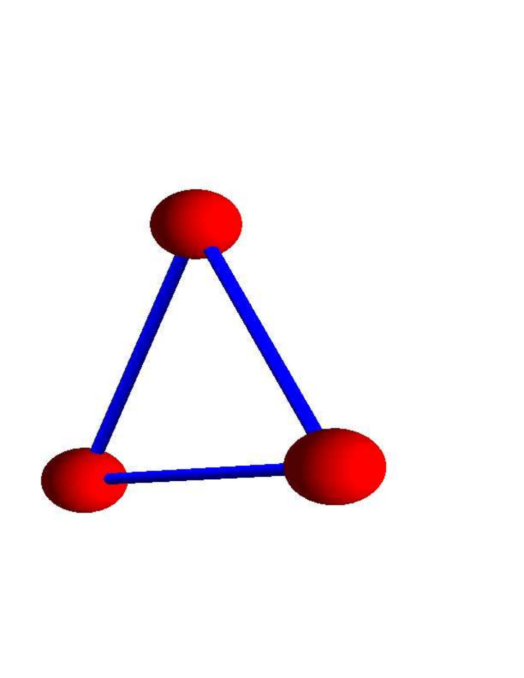
|
|---|---|---|---|
| is a -dimensional wheel graph with boundary. |

|
is a connected -dimensional graph without boundary. |

|
| Hessel’s example. is a union of two cyclic graphs. |

|
, the tetrahedron has dimension but has a boundary. |

|
| The utility graph is one dimensional |

|
A tri-pyramid construction of dimension 3 which contains |

|
| A figure 8 type graph is 1-dimensional but not smooth. |

|
A cube is a -dim graph. It is a graph theoretical polyhedron. |

|
|---|---|---|---|
| A stellated cube is a Catalan graph. |

|
The 3-cross-polytope = octahedron is the smallest 2-dim graph without boundary. |

|
| The 4-cross-polytope, the smallest 3 dimensional graph without boundary. |

|
The 5-cross-polytope is the smallest 4 dimensional graph without boundary. |

|
Many of the following examples are regular or semi-regular polyhedra in two and
higher dimension [19, 4]. Some of whom are Cayley graphs of finitely presented groups.
More examples can be obtained from constructions. We can borrow from any
construction known to manifolds. Here are examples of constructions which can be used to generate
new graphs from other graphs or from manifolds:
| Pyramid | add a vertex point and connect to all previous vertices |
|---|---|
| Bipyramid | add two vertices to get a dimensional graph |
| Joining | join d-dimensional graphs along dimensional subgraphs. |
| Identification | identify along isomorphic dimensional subgraphs. |
| Product | produces a dimensional graph after filling boundaries |
| Triangularization | produces d-dimensional graphs from -dimensional manifolds |
| Conway | kis, snub, truncate, gyro, propel etc to generate new graphs. |
The classical pyramid, bipyramid and prism constructions discussed for example in [10]
in the case of convex polytopes lead to higher dimensional regular polytopes.
The pyramid construction does not produce -dimensional
graphs unless the graph is a simplex.
If is a -dimensional graph with Euler characteristic , then the bi-pyramid construction is a -dimensional graph in the wider sense with Euler characteristic .
Proof.
The original graph is the unit sphere of both and . If is a vertex in the old graph , then its unit sphere is , where is the unit sphere of in the old graph. The new unit sphere is -dimensional. Since the unit spheres are either double pyramid constructions of old unit spheres or coincide with , the first claim follows by induction. If is two-dimensional with vertices, edges and faces, then has spaces and faces, edges and vertices. If the Euler characteristic of is , then the Euler characteristic of the bipyramid extension is . ∎
It follows that for every -dimensional graph there exists a -dimensional graph (in the wider sense without
any assumptions on the unit sphere) such that the unit sphere is .
The topology of the unit sphere is needed if we want to use only sphere quantities.
For -dimensional graphs without any assumptions on the unit spheres,
the unit spheres can be quite arbitrary. Classical differential geometry
motivates assumptions on the unit spheres for graphs. For radii smaller than
the injectivity radius of a Riemannian manifold , the geodesic sphere is a
topological sphere with Euler characteristic which
is for even and for odd . Its natural to assume this for graphs too.


Remark 1. The cross polytope in any dimension is obtained from the bipyramid construction
starting with the zero dimensional point. We can take any two dimensional graph ,
add two points and get a three dimensional graph
etc.
Remark 2. After repeating such a construction, we have a -dimensional
graph with the same Euler characteristic. It can be repeated. To get a -dimensional
connected graph with Euler characteristic , start with a two dimensional graph with
this Euler characteristic, then do the bi-pyramid construction 98 times.
Given two dimensional graphs and assume that there are dimensional spheres with a graph isomorphisms . The joined graph by identifying points along is a -dimensional graph of Euler characteristic .
Proof.
We have to show that (i) each unit sphere in the new graph is a -dimensional graph, that (ii) each unit sphere has Euler characteristic and (iii) that for the new graph. The statement is true for one dimensional graphs. We use induction to verify it in higher dimensions. Statements (i),(ii) need only to be proven for points on or . The surgery has induced a smaller dimensional surgery for the unit spheres along dimensional graphs. By induction, the dimension is correct. The Euler characteristic of each unit sphere stays because the is the same than the Euler characteristic of union of the complement with the boundary. The joining does not change the property that every face of a -dimensional simplex is connected to a -dimensional simplex. Therefore stays true. Finally, the Euler characteristic formula for the entire follows because the simplices add up, we remove two balls with Euler characteristic and double-count the intersection . ∎
For example, joining two simply connected two-dimensional graphs of Euler characteristic
along a one-dimensional graph has Euler characteristic . The new graph is still simply
connected. If we join two -dimensional doughnut graphs of Euler characteristic
along a circle, we get a graph with Euler characteristic .

Also when identifying points of the graph, we get a new graph of the same dimension in general:
given a graph and assume that there are -dimensional spheres
for which and such that there is a graph isomorphism: .
By identifying points along , we get a new -dimensional graph of Euler
characteristic .
For two-dimensional graphs, this identification corresponds to adding ”handles”
so that the new graph has Euler characteristic .
Finally, one could ask about using random processes to generate d-dimensional graphs. Among all undirected graphs with vertices the -dimensional ones of course have probability which goes to zero for . But we can generate graphs by ”aggrevation” starting with a ball of radius one, adding more balls. For two-dimensional graphs we will end up with a planar graph which when finite, has Euler characteristic . Picture (5) gives an example.
| polyhedron | vertices | edges | faces | curvatures | |
|---|---|---|---|---|---|
| octahedron | 6 | 12 | 8 | 2/6 | |
| icosahedron | 12 | 30 | 20 | 1/6 | |
| stellated cube | 14 | 36 | 24 | 0,1/3 | |
| drilled cube | 16 | 48 | 32 | 0 | |
| drilled stellated cube | 16 | 96 | 64 | 1/3,-1/3 |
| cube | 1 |

|
| tetrahedron | 3 |

|
| octahedron | 2 |

|
| icosahedron | 2 |

|
| dodecahedron | 1 |

|
| stellated cube | 1 |

|
| stellated dodecahedron | 2 |

|
| drilled cube | 2 |

|
| drilled stellated cube | 2 |

|
| stellated icosahedron | 2 |

|
The dimension of a vertex is the average dimension of its unit sphere plus 1.
The dimension of the graph can then be defined as the average of the dimensions of its points.
Figure 7 shows the dimensions for the 13 Archimedean solids and their
duals, the Catalan solids.

|

|

|
| (2,-4) | (1,-60) | (1,-24) |

|

|

|
| (2,-10) | (3/2,-40) | (3/2,-16) |

|

|

|
| (2,-4) | (2,-10) | (5/3,-4) |

|

|

|
| (5/3,-10) | (1,-30) | (1,-12) |

|
||
| (5/3,-2) |

|

|

|
| (1,-10) | (2,2) | (2,2) |

|

|

|
| (1,-28) | (1,-58) | (1,-22) |

|

|

|
| (1,-22) | (1,-58) | (3,2) |

|

|

|
| (3,2) | (2,2) | (2,2) |

|
||
| (3,1) |
For two-dimensional graphs , positive curvature means that the degree is or . Because , there are only finitely many positive curvature graphs. We have a list in two dimensions and know therefore - the proof is left out here - that only finitely many -dimensional graphs exist for which all sectional curvatures - curvatures of two dimensional subgraphs - are positive. For two dimensional graphs, the genus defined by is the number of holes in the graph. For a two-dimensional graph , the values of and determine the edge and face cardinalities by and .
| octahedron |

|
|---|---|
| 10 hedron |

|
| 12 hedron |

|
| 14 hedron |

|
|---|---|
| 16 hedron |

|
| icosahedron |

|
5.2. Three dimensional graphs
The Euler curvature form is identically zero for three-dimensional graphs. As a consequence of Gauss-Bonnet-Chern, the Euler characteristic of a three dimensional graph is zero. This is a discrete version of Poincarè’s result that odd dimensional compact manifolds have zero Euler characteristic.
Corollary 4.
The Euler curvature form is identically zero for three dimensional graphs.
Even so, this is a special case of the theorem, we look at the calculation in three dimensions:
Proof.
If the number of three dimensional chambers of the graph, the Euler characteristic of a three dimensional graph is
The hyper relations are and , where the number of vertices, edges and faces on the sphere . The Euler relation on each sphere is . The transfer relations
give from the formula
Adding this together with provides
and so
The hyper surface relation shows that this is zero. ∎
Example 3.1. For a octahedral tessellation of a 3D torus, we confirm zero curvature everywhere.
The Euler characteristic is .
Example 3.2. For a 3-dimensional tetrahedron , we have and the curvature
is constant 0. Note that this case is not covered by the theorem because the unit sphere of any point
of is which is a two-dimensional graph with Euler
characteristic which is different from the required.
Example 3.3. A 4-cross polytope is a bi-pyramid constructed from an octahedron. It is also called .
Each unit sphere has 6 points and is a regular octahedron with edges and faces.
For a realization of the 4-cross polytope in , two points are connected if they have distance
. The unit sphere at a point consists of the 6 points
, which form an
octahedron with .
| vertices | ||
|---|---|---|
| edges | ||
| faces | ||
| chambers |
We check in all these examples that the
curvature form is .


Example 3.4. The 600 cell is a regular polytope with 120 vertices.
We see from the complete list of all 6 regular polytopes in that besides the just discussed 16-cell, that the
600 cell is the only remaining three dimensional graph which corresponds to a regular convex
polytope in 4 dimensions. Its unit sphere is a regular icosahedron with edges and faces.
| 5 cell of dim 4 with tetrahedron as sphere |

|
|---|---|
| 8 cell of dim 1 with 4 points as sphere |

|
| 600 cell of dim 3 and icosahedron as unit sphere |
|
| 16 cell of dim 3 with octahedron as sphere |

|
|---|---|
| 24 cell of dim 2 and cube as unit sphere |

|
| 120 cell of dim 1 and 4 discrete points as unit sphere |

|
Example 3.5. The hypercube is usually realized in .
This 8-cell or tesseract is initially one-dimensional since each unit sphere consists
of 4 disjoint points. It has initially 16 vertices, 32 edges, 24 faces and 8 cells, the Euler characteristic is
. We add on each of the 24 faces an additional vertex and connect it to the four old vertices. Then
we add 8 more vertices at the center of the cells and connect it to the 14 neighboring vertices. Now, we have a three
dimensional graph. The new data are .
The unit spheres consist of 24 stellated two-dimensional cubes or octahedra. The octahedra are the
unit spheres of the newly added faces, while the stellated cubes are centered at the original cell centers or vertices.
The Euler curvature form for is zero.
For the octahedron we have and for the stellated cube, we have and .
Example 3.6. The 24 cell has 24 vertices, 96 faces, 96 edges and 24 cells.
It is a selfdual graph but only two dimensional, because each unit sphere is a cube which is
one dimensional. Again, we can produce a three dimensional graph from it by adding the centers
of each square. Now the unit spheres are stellated cubes with vertices, edges and and faces.
The Euler curvature form of the three dimensional completion of the 24 cell is still zero.
The 24 cell can be used to tesselate four dimensional space
in an icositetrachoric honeycomb. Also this is a self-dual situation and by doing identifications
we can use this to generate triangularizations of the three dimensional torus.
Note that what we would consider three dimensional are denoted four dimensional polytopes because they are are polytopes realized in . Or polyhedra in are called Examples of Archimedean polytopes are illustrated in [13]. We think of them as three dimensional because a stellation or snub operations produce three dimensional graphs from them.
5.3. Four dimensional graphs
Since the curvature form vanishes identically in three dimensions,
the four dimensional situation is the first really interesting case for Gauss-Bonnet-Chern
beyond two dimensions. Assume is a vertex in a four dimensional graph .
Let denote the number of vertices in , let the number
of edges in , let the number of faces in and let
denote the number of three dimensional chambers in .
The transfer equations are
| sphere vertices edges in graph | edges are counted 2 times | |
| sphere edges faces on graph | faces are counted 3 times | |
| sphere faces chambers on graph | chambers are counted 4 times | |
| sphere chambers graph spaces | spaces are counted 5 times |
Here is the computation done in the proof of the theorem in the special case . Similarly as any face is bordered by edges, every chamber is border by faces, every hyper chamber is bordered by chambers which each are counted twice. We have therefore the hyper relations . The hyper relations on each three dimensional sphere are . The Euler characteristic on the three dimensional sphere is zero: . Use the transfer relations with
to get
Add
to get
With we end up with
Example 4.1. The 4-dimensional simplex has the data
. The Euler curvature form takes the value
everywhere. Since there are 5 vertices, we confirm
.
Example 4.2. The four-dimensional cross-polytope or orthoplex
can be realized as a regular convex polyhedron in . It is dual to the 5-cube, the penteract.
From the simplex data
| vertices | |
|---|---|
| edges | |
| faces | |
| chambers | |
| spaces |
we get .
Now, each unit sphere has vertices which form a 4-cross polytope. The Euler curvature form
is constant .
There are 10 vertices and the total Euler curvature form is which agrees with
the Euler characteristic.


Example 4.3. The 4-dimensional cube realized in as is one-dimensional because every vertex has a sphere which consists of isolated points. The cube has 10 spaces: when realized in as above, the coordinates choice to or determines these chambers centered at
then chambers where two of the coordinates are nonzero
and faces where 3 of the coordinates are nonzero and
edges (fix 4 of the coordinates) and vertices:
The Euler characteristic is .
| vertices | ||
|---|---|---|
| edges | , etc | |
| faces | etc | |
| chambers | ||
| spaces |
In order to make it a 4-dimensional graph, we first stellate each of the
two dimensional faces, then each three dimensional chambers, then each of the 4 dimensional
hyper chambers. We get concrete vertices by averaging over other vertices:
| Original vertices | ||
|---|---|---|
| edge centers | etc | |
| face centers | etc | |
| chamber centers | etc | |
| space centers | etc |
The stellated cube is seen in Figure (11).
The Euler characteristic is .
In this case, the Euler form curvature function
is non-constant:
| 80 | 10 | 34 | 48 | 24 | 2/15 |
| 40 | 16 | 64 | 96 | 48 | -1/15 |
| 32 | 30 | 150 | 240 | 120 | 0 |
| 10 | 48 | 240 | 384 | 192 | -3/5 |
The total curvature is , which agrees with the
Euler characteristic .
Example 4.4. The 4 dimensional octahedron is obtained from the 3-dimensional octahedron with
the bi-pyramid construction. Lets compute the curvature for a four dimensional
graph which is obtained from a 3 dimensional graph by the bi-pyramid construction.
We have where are
the vertex, edge and face cardinalities of the three dimensional graph .
If is in which has a unit sphere which is a two dimensional closed graph
with cardinalities . Then and so that
. Because for two dimensional graphs with Euler characteristic ,
we have and , we see that , where are the number of vertices in
the two dimensional graph , the unit sphere of in .
Assume is a -dimensional graph with vertices, edges and faces and if is
the cardinality of the unit sphere, then the Euler form of the four dimensional bipyramid construction is
and for .
Example 4.5. For the dimensional cross polytope with vertices, where for the unit sphere
, we have at every old point and for the newly added points.
Example 4.6. We see that if the three dimensional graph has two dimensional unit spheres with more than 12 points, then the Euler curvature form of the four dimensional graph is negative on the additional points . It follows that if we know the eigenvalues of the adjacency matrix of the graph and if we know the degree matrix then we know the Euler curvature form of from the spectral data. The reason is that we know and and and so the Euler curvature form.
5.4. Five dimensional graphs
In 5 dimensions the transfer equations are
We know
| 6 t = 2 s | 5D paces are bordered by 6D spaces counted twice |
| 5 S = 2 C | the hyper surface relation on the sphere |
and
| Euler characteristic | |
| Euler characteristic of 4D sphere |
Filling in the transfer equations into the Euler characteristic and
dividing the equation for by 2 gives
Adding them up and using gives
While we know that the Euler characteristic is zero, it is not clear whether for any dimensional graphs
is necessary. In other words, is the Euler curvature form zero in general in five or any odd dimensions?
Example 5.1. For a 5-dimensional simplex, we have .
The Euler curvature form is constant zero here: . This is not a graph as defined here because
the unit spheres are 4-dimensional simplices of Euler characteristic .
Example 5.2. The 5 dimensional octahedron is also called 6-cross polytope and is dual to the 6-cube,
the ”hexeract”.
| Vertices | |
|---|---|
| Edges | |
| Faces |
| chambers | |
|---|---|
| spaces | |
| halls |
Its Euler characteristic is as for any dimensional spherical graph.
We have and .
Example 5.3 The 5 dimensional rectified hexeract is an example of an uniform 6-polytop which
can be built in by taking all points as well as all
cyclic permutations and connecting two vertices if the distance is .
The graph obtained has vertices and edges.
Each unit sphere is a union of two disjoint four dimensional disjoint ’s.
While for all , these spheres are not connected and the graph does not
satisfy the assumptions we have imposed.
Example 5.4. The -dimensional stellated cube is obtained by
stellating the halls, the four dimensional
chambers, the three dimensional spaces and faces.
Together with the initial vertices, his gives a total of
vertices.
The fully triangulated graph is now dimensional and has edges.
The original cube is a dimensional polytop in a graph theoretical sense.
There are different type of vertices in . Their unit spheres
are four dimensional graphs with the following data:
| spheres | V | E | F | C | H | K |
|---|---|---|---|---|---|---|
| 64 | 62 | 540 | 1560 | 1800 | 720 | 0 |
| 240 | 18 | 96 | 224 | 240 | 96 | 0 |
| 160 | 20 | 126 | 324 | 360 | 144 | 0 |
| 60 | 50 | 336 | 864 | 960 | 384 | 0 |
| 12 | 162 | 1440 | 4160 | 4800 | 1920 | 0 |
This example was realized in the computer to check whether is identically zero. While in the continuum, the Euler curvature is not defined in odd dimensions, it is here in the discrete, where could a priori be interesting. It seems that is identically zero for odd dimensional graphs however.
5.5. Six dimensional graphs
Lets start with the computation again in the dimensional case:
From we get
Now use the hyper relations and
to get
Example 6.1. The dimensional octahedron is also called 7-crosspolytope. It is a -polytope which can be realized as a convex solid in with vertices etc. It is the analogue of the octahedron. The unit spheres are -cross polytopes, which in turn then have -cross polytopes as unit spheres etc, until we reach the -cross polytope, the square.
| vertices | |
|---|---|
| edges | |
| faces | |
| chambers | |
| spaces | |
| 5-halls | |
| 6-halls |
Its Euler characteristic is as for any -dimensional spherical graph.
We have and .
There are 14 vertices and the total curvature is
and agrees with the Euler characteristic.
Example 6.2 The rectified -demicube or demihepteract is realized with coordinates with an even number of . The graph is not dimensional however since the unit sphere of a point of the unit sphere of a point on that unit sphere can become disconnected.
5.6. Seven dimensional graphs
For seven dimensional graphs, the Euler curvature form is , where is
the number of three dimensional chambers, is the number of four dimensional spaces and
the number of dimensional halls in . Also here, if the graph is a triangularization
of a dimensional orientable manifold, then the sum of the curvatures is zero by Poincaré duality.
Example 7.1. The -crosspolytope can be realized as a convex polyhedron in . It
has Euler characteristic . Since all unit spheres are isomorphic graphs, the curvature form has to be zero
everywhere. Here are the simplicial subgraphs of :
| Vertices | |
|---|---|
| edges | |
| faces | |
| chambers |
| spaces | |
|---|---|
| 5-halls | |
| 6-halls | |
| 7-halls |
Its Euler characteristic is as for any odd dimensional spherical graph.
We have and . The total curvature is
and agrees with the Euler characteristic.
We do not have an example yet of a 7-dimensional graph, where is different from zero at some vertices.
References
- [1] S.-S. Chern. A simple intrinsic proof of the Gauss-Bonnet formula for closed Riemannian manifolds. Annals of Mathematics, 45, 1944.
- [2] F.R.K. Chung. Spectral graph theory, volume 92 of CBMS Regional Conference Series in Mathematics. AMS, 1997.
- [3] R. Cohen and S. Havlin. Complex Networks, Structure, Robustness and Function. Cambridge University Press, 2010.
- [4] H.S.M. Coxeter. Regular Polytopes. Dover Publications, New York, 1973.
- [5] K.S. Thorne C.W. Misner and J.A. Wheeler. Gravitation. Freeman, San Francisco, 1973.
- [6] H.L. Cycon, R.G.Froese, W.Kirsch, and B.Simon. Schrödinger Operators—with Application to Quantum Mechanics and Global Geometry. Springer-Verlag.
- [7] S. Devadoss and J. O’Rourke. Discrete and Computational Geometry. Princeton University Press, 2011.
- [8] R. Engelking. Dimension Theory. North-Holland Publishing Company, 1978.
- [9] M. Gromov. Hyperbolic groups. In Essays in group theory, volume 8 of Math. Sci. Res. Inst. Publ., pages 75–263. 1987.
- [10] B. Grünbaum. Convex Polytopes. Springer, 2003.
- [11] Y. Higuchi. Combinatorial curvature for planar graphs. J. Graph Theory, 38, 2001.
- [12] W. Hurewicz and H. Wallman. Dimension Theory. Princeton mathematical series. 1941.
- [13] C. Goodman-Strauss J.H. Conway, H.Burgiel. The Symmetries of Things. A.K. Peterse, Ltd., 2008.
- [14] O. Knill. A discrete Gauss-Bonnet type theorem. Elemente der Mathematik (to appear), 2011. http://arxiv.org/abs/1009.2292.
- [15] J.M. Lee. Riemannian manifolds, volume 176 of Graduate Texts in Mathematics. Springer-Verlag, New York, 1997. An introduction to curvature.
- [16] J.R. Munkres. Topology, a first course. Princeton Hall, New Jersey, 1975.
- [17] A.R. Pears. Dimension Theory of General Spaces. Cambridge University Press, London, New York, 1975.
- [18] S. Rosenberg. The Laplacian on a Riemannian Manifold, volume 31 of London Mathematical Society, Student Texts.
- [19] L. Schlafli. Theorie der Vielfachen Kontinuität. Cornell University Library Digital Collections, 1901.