Linear Polymers in Disordered Media
– the shortest, the longest and the mean(est) SAW on percolation clusters
Abstract
Long linear polymers in strongly disordered media are well described by self-avoiding walks (SAWs) on percolation clusters and a lot can be learned about the statistics of these polymers by studying the length-distribution of SAWs on percolation clusters. This distribution encompasses to distinct averages, viz. the average over the conformations of the underlying cluster and the SAW-conformations. For the latter average, there are two basic options one being static and one being kinetic. It is well known for static averaging that if the disorder of the underlying medium is weak, this disorder is redundant in the sense the renormalization group, i.e., differences to the ordered case appear merely in non-universal quantities. Using dynamical field theory, we show that the same holds true for kinetic averaging. Our main focus, however, lies on strong disorder, i.e., the medium being close to the percolation point, where disorder is relevant. Employing a field theory for the nonlinear random resistor network in conjunction with a real-world interpretation of the corresponding Feynman diagrams, we calculate the scaling exponents for the shortest, the longest and the mean or average SAW to 2-loop order. In addition, we calculate to 2-loop order the entire family of multifractal exponents that governs the moments of the the statistical weights of the elementary constituents (bonds or sites of the underlying fractal cluster) contributing to the SAWs. Our RG analysis reveals that kinetic averaging leads to renormalizability whereas static averaging does not, and hence, we argue that the latter does not lead to a well-defined scaling limit. We discuss the possible implications of this finding for experiments and numerical simulations which have produced wide-spread results for the exponent of the average SAW. To corroborate our results, we also study the well-known Meir-Harris model for SAWs on percolation clusters. We demonstrate that the Meir-Harris model leads back up to 2-loop order to the renormalizable real world formulation with kinetic averaging if the replica limit is consistently performed at the first possible instant in the course of the calculation.
pacs
64.60.ah, 61.41.+e, 64.60.al, 64.60.aeI Introduction
Linear polymers in disordered media have been an important topic for experimental and theoretical study for more than 20 years [1]. It is a well known fact that that the universal scaling properties of linear polymers in strongly disordered media are well described by the statistics of self-avoiding-walks (SAWs) on percolation clusters. Usually, the term SAW implicitly refers to a mean or average SAW for which an average is taken over the number of steps or intrinsic lengths of all self-avoiding walks with a specified Eukledian start-to-end distance or, respectively, over the start-to-end distances of all self-avoiding walks with a specified intrinsic length. However, there are other SAWs that are equally interesting. Most notably, there is the shortest and longest SAW for which the intrinsic length for given terminal-separation is shortest and longest, respectively. On critical percolation clusters, all these SAWs are fractals, i.e., their masses (which are proportional to their intrinsic lengths, of course) as functions of the start-to-end distance scale with non-integer scaling exponents. Interestingly, however, it turns out that the mean SAW is more than just a simple fractal – it is a multifractal. On critical percolation clusters, the statistical weights of the elementary constituents (bonds or sites) are non-trivial, and an entire family of multifractal scaling exponents is required to characterize the distribution of these weights through its moments.
Although the last 2 decades have brought great advancement in the understanding of linear polymers in disordered media, there are certain problems that have caused enduring controversy. For example it turned out that the famous Meir-Harris (MH) model [2] which has long been standing as the only existing field theoretic model for studying average SAWs on percolation clusters has trouble with renormalizability [4, 3]. Another example is the puzzling fact that sophisticated numerical simulations by various groups have produced widespread results for the scaling exponent describing the mean length of the average SAW, see [1].
In this paper, we highlight that one has to be careful about the notion of average SAW if the disorder of the underlying medium is strong. Namely, there are essentially two qualitatively different ways of averaging over all SAWs between two connected sites for a given random configuration of a diluted lattice, one being static and the other being kinetic. It is well known that the exponent in a non-random medium is the same for static and kinetic averaging [5, 6, 7, 8], and that weak disorder of the medium in redundant in the sense of the renormalization group (RG) if static averaging is used [9]. Below, we employ dynamical field theory to demonstrate that the same holds true for kinetic averaging. To discuss the effects of strong disorder, we present a renormalizable field theory for SAWs on percolation clusters based on the random resistor network (RRN). We use this theory to calculate the scaling exponents of the shortest, the longest and the average SAW as well as the entire family of multifractal exponents for SAWs on percolation clusters. This theory demonstrates that kinetic and static averaging may lead to very different results if the random medium is at the percolation point. Within the real-world interpretation of Feynman-diagrams, static averaging leads to non-renormalizability, and hence we argue that the statistics of linear polymers in disordered media may not have anasymptotic scaling limit, when static averaging is used. Because the static average has been used in many simulations, this might explain why the numerical results for are so wide spread. In fact, recent simulations by Blavatska and Janke [10, 11] using kinetic averaging are in excellent agreement with our theoretical results. To further corroborate our findings and to shed some light on them from a different angle, we include a discussion of the MH model in the context of kinetic vs. static averaging. A brief account of the work presented here has been given previously in Ref. [12].
II Observables and averages
The fundamental question addressed in this paper is that of the scaling behavior the length of a (shortest, longest or mean) SAW on a percolation cluster when averaged over all cluster conformation. To this end, one can either consider the scaling of the mean Euclidian distance between the starting point and a random endpoint of an SAW of length ,
| (1) |
or one can study averages over the random length of a SAW (which is proportional to the number of monomers, the intrinsic length or the mass of the corresponding polymer) between a pair of sites as a function of their Euklidian distance . The latter approach is more convenient from the standpoint of field theory [2], and we will take it here.
Let be the pair connectedness indicator function which is unity if and are connected in the given random configuration and zero otherwise. Let be the generating function of the SAWs with length belonging to the bundle of all SAWs starting at and ending at both on cluster . This generating function can be written as
| (2) |
where is a weight function that depends on the averaging procedure one uses and which, of course, has to satisfy . Special cases are if is either the shortest or the longest SAW belonging to the bundle . The perhaps most basic averaging procedures are either static, i.e., all the ’s belonging to are weighted equally, , or kinetic, i.e., a given earns a factor contributing to at each ramification where other SAWs from the bundle split off and which, in general, leads to different weights for different ’s.Note that in kinetic averaging, the probabilities satisfy the additivity property when two SAWs and are identified, e.g., in a coarse-graining procedure. To the contrary, this is not the case in static averaging because the number changes when SAWs are identified, and this fact leads to trouble when coarse-graining procedures are applied spatial inhomogeneous fractals like the backbone of a percolation cluster as they are in renormalized field theory.
In terms of the generating function, the mean length of the SAWs is given by
| (3) |
where denotes an average over the configurations in which each bond is occupied with probability . At criticality, one expects scaling behavior of the mean length of long polymer chains,
| (4) |
For kinetic averaging, in particular, the critical value of is zero.
It is well known that multifractality can arise when physical processes unfold on fractals such as critical percolation clusters. Typical examples are electrical conduction on RRNs [13, 14, 15, 16, 17, 18] and random resistor diode networks [19, 20] where the distribution of currents flowing through the bonds is multifractal, i.e., is characterized by an infinite set of critical exponents which are not related in a simple linear or affine fashion. It turns out that the situation is similar for SAWs on percolation clusters, where the moments
| (5) |
with the length of bond and
| (6) |
the statistical weight of bond with if belongs to the SAW and if it does not, probe distinct substructures of the underlying percolation cluster and hence the average
| (7) |
leads to an infinite family of multifractal exponents :
| (8) |
One has the special cases , , and where is the fractal dimension of the backbone, is the fractal dimension of the red (simply connecting) bonds, and is the percolation correlation length exponent.
III SAWs in disordered media as a kinetic process – the effects of weak disorder
In this section we briefly discuss the effects that weak disorder of the underlying medium has on the statistics of SAWs. For static averaging over SAW conformations, it well known that this disorder is redundant in the sense of the RG, i.e., it affects only non-universal quantities (in annealed as well as in quenched disorder-averages) although a naïve application of the Harris criterion [9] apparently signals its relevance. This redundancy can be shown by introducing non-correlated quenched disorder into the usual -field theory of a -component order parameter which, when the replica trick with -fold replication is used to facilitate averaging over the quenched disorder, generates the statistics of SAWs with static averaging via the limits and . Here, we are interested mainly in kinetic averaging, and hence it is of some interest to demonstrate that this redundancy also holds for this type of averaging. A field theory for kinetically generated SAWs in ordered media has been formulated by Peliti more than twenty years ago [6]. Here, we introduce a dynamical field theoretic model for kinetically generated SAWs in disordered media, and we utilize this model to discuss the effects of weak disorder. To set the stage, we first introduce reaction diffusion processes that model SAWs in disordered media as a kinetic process and then we jump to the dynamical response functional for these processes. Additional background and some details of its derivation using the creation-destruction operator formalism are given in Appendix A. It should not go un-noted that this description of SAWs in disordered media as a kinetic process completely avoids using the replica trick as well as the zero-component-limit and hence all the potential difficulties associated with these limits.
On a very basic and intuitive level, kinetic SAWs in disordered media can be described by a set of simple diffusion and reaction processes. As in the problem of Brownian walks, the walkers hop on a -dimensional cubic lattice from a site to a neighboring one . This is described by a random process
| (9) |
where denotes a random walker at , and is the hopping rate. Self-avoidance is introduced by production of markers at , and destruction of the walkers by interaction with a marker
| (10a) | ||||
| (10b) | ||||
where and are reaction rates. In addition to these processes, there is quenched disorder modelled by static traps with a random distribution , and this disorder acts on the walkers via a destruction process with rate
| (11) |
Due to the markers and the traps, walkers living at time should avoid sites that they have visited at times as well as sites which are locations of traps.
These diffusion and reaction processes can be condensed into a field theoretic functional following the work of Peliti. A series of steps which are sketched in the Appendix leads to the dynamical response functional
| (12) |
is a field that has its origin in the variable and encodes the random position of a walker at time according to the above reactions. Its mean value is the probability density finding a walker at these coordinates. is the corresponding response field that creates a walker at position at time . The dynamical response functional is invariant under the duality transformation . is the usual kinetic coefficient. The dependence of on the disorder is hidden in the parameter and in the coupling constant . The latter consists of two parts: a positive part stemming from the self-avoidance and an additional negative part stemming from the disorder. Note that the fact that disorder and self-avoidance generate the same type of coupling in the field-theoretic functional makes the Harris criterion inapplicable for the problem at hand.
Analyzing the RG flow, it turns out that the fixed point value of which corresponds to the limit of asymptotically large SAWs is independent of the nonuniversal value of and hence of the disorder fluctuations. Because we are mainly interested in this limit, we can assume that the sole remaining disorder-dependence rests in . However, we can eliminate from the dynamical response functional by letting and . This implies that the disorder-averaged Greens functions – the probability densities for finding walkers at positions at times if they are created at positions at times , respectively –
| (13) |
where denotes the cumulants with respect to the Boltzmann weight and denotes disorder averaging, are of the form
| (14) |
where the index indicates the Greens functions without any disorder. The differences are proportional to the lengths of the corresponding SAWs, and hence, the exponential factors correspond to a change in the non-universal fugacities in the statistics of the SAWs. Thus, Eq. (14) reveals that all universal properties remain unaffected by disorder. This establishes that the universal properties of kinetically generated and averaged SAWs are independent of weak disorder as their statically averaged counterparts are [9].
IV Nonlinear random resistor networks
The RRN is a variant of the usual percolation problem where occupied bonds are viewed as resistors and open bonds are viewed as insulators. Here, we consider a nonlinear generalization nRRN of the RRN for which it is well known that the total resistance between 2 points becomes proportional to the length of the shortest and longest SAW between those 2 points, respectively, for specific limits of the nonlinearity. In previous work [21, 23, 24, 18], we have shown that the Feynman diagrams for RRNs (including their nonlinear generalization) have a real-world interpretation, i.e., they can be considered as being resistor networks themselves. Based on this real-world interpretation, we here develop an intuitive and powerful field-theoretic method to calculate the mean length and multifractal moments of SAWs on percolation clusters.
To be specific, we consider a -dimensional lattice where each bond is randomly occupied with probability by a conductor or empty with probability . At each lattice side there is a voltage . The voltage drop at a bond between sites and obeys a generalized Ohm’s law [25]
| (15) |
with a bond resistance . Equivalently, with the current across the bond is given by
| (16) |
where is the non-linear conductance of the bond. We restrict ourselves in the following to the case that all occupied bonds have identical elementary conductances , and the conductances of the unoccupied bonds are zero. The currents are conserved at each site and obey Kirchhoff’s first law
| (17) |
where is an external current flowing into site . If there are only two ports and , these currents are given by , where is the current resulting from the voltage difference between the two ports. The electrical power dissipated in the network is given by the bilinear form
| (18) |
where the two last equalities follow from Ohm’s law, Eqs. (15) and (16). Using Eq. (17), one has
| (19) |
in the two-port case, where denotes the total resistance of the network between the two ports. Blumenfeld et al. [26] have shown that the special values , , , , and describe physically relevant geometric properties of the diluted lattice. In particular, it is easily demonstrated that for the internal currents at each ramification flow only in the direction of the highest () or the lowest () voltage gradient (electromotorical force) thereby mapping out the shortest or the longest SAW between the 2 terminals, respectively. As a consequence, the resistance is proportional to the length of shortest or longest SAW between and for or , respectively. We will use this fact for calculating the average length for these SAWs via calculating the total nonlinear resistance averaged subject to the condition, that the two ports are on the same cluster,
| (20) |
At criticality, the average total nonlinear resistance obeys the power law
| (21) |
which will allow us to extract the SAW exponents for the shortest and the longest SAW simply by taking the appropriate limit with respect to .
As far as the average SAW is concerned, the situation is somewhat more subtle. Obviously, the average length of the average SAW lies in between the average length of the shortest and the longest SAW, which are, of course, very different. Since average SAW sits somewhere in this discontinuity at , it is not known how to extract its average length from the nRRN by a limit taking. To overcome this problem, we developed the idea to study the average SAW by using the real-world interpretation [23, 24, 18, 33] of Feynman diagrams which we will discuss in detail in the following section. For studying SAWs on percolation clusters, we extend the real-world interpretation originally developed for studying electrical transport on RRNs in that we put SAWs on Feynman diagrams. As we will explain in detail below, the task of calculating the average length of SAWs on percolation clusters then in essence reduces to calculating the average length of SAWs on Feynman diagrams. For the average SAW in particular, this approach avoids the aforementioned problems associated with taking a limit in
The resistance can be obtained by solving the circuit equations (16), (15), and (17). The circuit equations can be viewed as a consequence of the variation principle
| (22) |
where the power is expressed purely as a function of the set of all voltages , see Eq. (18). Obviously the network may contain closed loops. Suppose there is a complete set of independent currents circulating around these loops. Using Kirchhoff’s first law (17) and Eq. (18), one can express the electrical power entirely as a function of the external current and the set of loop currents . Then, one readily obtains Kirchhoff’s second law as a consequence of the second variational principle
| (23) |
This equation is used in the following to determine the loop currents as linear functions of the external current . For , the variation principle (23) has a unique solution which corresponds, of course, to the global minimum of the power . Without ambiguity, this solution leads to where denotes the length of the shortest SAW (the chemical length). For , the situation is less straightforward. There exist in general several solutions which are all local maxima of the power [26]. Only if one selects the solution corresponding to the global maximum of , one gets the length of the longest SAW via . As mentioned above, the average length of the average SAWs has to lie somewhere in the interval between these two extremal values and for a correct interpretation of , it seems natural to demand that it produces the length of the average SAW, .
V Harris model
A field theory for the non-linear random network was set up by Harris [27] in analogy to the field theory of the linear case [28, 30]. The network is replicated fold: . One considers the correlation function of with complex currents :
| (24) |
Here , and is the usual configuration dependent normalization. In order to be well defined, the integrations over replicated voltages are augmented with extra weight factors . Physically, these weights correspond to grounding all sites via unit capacitors. In this picture, with corresponds to the frequency of the voltages.
Because the electrical power depends only on voltage differences, the integration over the mean voltage of each independent cluster of connected conductors leads to current conservation for this cluster in the limit . It follows that if the ports and are connected. However in the case that and are not connected, there arise factors , where is some positive constant, which go to zero in the limit . Here, the condition is essential. Then, as the result of this integration, the pair connectedness indicator function of the two ports is automatically generated along with other factors which go to one in the limit . Following the work of Harris [27], the integration over the voltage differences can now be done by the saddle-point approximation if we chose with under the conditions and which indeed can be satisfied simultaneously in the replica limit . Note that the saddle-point equations are identical with the variation principle stated in Eq. (22). Thus, the saddle-point is determined by the solution of the circuit equations (15), (16), and (17), and according to Eqs. (18) and (19), we obtain
| (25) |
where and where we dropped a factor that goes to 1 in the limit . Hence, is the cumulant generating function for the resistance between the connected ports and . is proportional to the elementary resistance . Hence, is the correlation (connectedness) function of the percolation problem.
To safely exclude from the theory it is useful to resort to a lattice regularization of the voltage-integrals [29]. One switches variables to and taking discrete values on a -dimensional torus, i.e. and are chosen to be -dimensional integers with and , . is a redundant variable with arbitrary scaling behavior.
After discretization there are independent state variables per lattice site, and one introduces the Potts-spins
| (26) |
subject to the condition . It is essential as we already have remarked above that the limit is the first of all involved limits and, in particular, has to be taken before .
The replication procedure leads to the effective Hamiltonian
| (27) |
which may be expanded in terms of or, equivalently,
| (28) |
where is the (discrete) gradient in the replica space. Next the kernel is expanded in the limit of large conductance (small resistance
| (29) |
with . Therefore, in the limit we have , and we recover the -state Potts-model which describes percolation in the limit .
By choosing the redundant variable appropriately, one can show that all terms in Eq. (29) with are irrelevant in the sense of the renormalization group. The merely lead to corrections to the leading scaling behavior that have been calculated for the linear RRN, , in Ref. [32]. They do not lead, however, to a family of crossover exponents as erroneously concluded in Refs. [30, 31]. Bluntly stated, RRNs are multifractal but they are not multicritical.
VI Field theory
To set up a field theoretic Hamiltonian , one proceeds with the usual coarse graining step and replace the Potts-spins by the order-parameter field defined on a -dimensional spatial continuum. Constructing all possible relevant invariants of the symmetry transformations of the model, performing a gradient expansion and discarding all irrelevant terms, one arrives at the Hamiltonian
| (30) |
Here and are the strongly relevant critical control parameters and . For which corresponds to , one has full Potts-symmetry, that is invariance under all permutations of the symmetric group . The discrete states of the order-parameter field transform as the fundamental representation of this permutation group. This fact is crucial because it is the irreducibility of this representation that ensures that there is only one invariant second and only one invariant third order coupling with one unique relevant control parameter and coupling constant , respectively.
Now we set up a diagrammatic expansion. Contributing elements are the vertex with weight and the Gaussian propagator which reads
| (31) |
in Fourier space. This inclusion-exclusion equation shows that the principal propagator decomposes into a propagator carrying (conducting) and one not carrying (insulating). This fact allows for a schematic decomposition of the principal diagrams into sums of RRN-like conducting diagrams consisting of conducting and insulating propagators, see Fig. 1. Note that, like the momenta , the (imaginary) currents are conserved at each vertex of the conducting diagrams. For actual calculations, it is more practical to use continuous rather than discrete replica currents . Once the decomposition is done, it is save to switch back to integrations over loop replica currents using
| (32) |
where the limit is understood.

The Feynman diagrams resulting from the decomposition have a simple and intuitive interpretation [21] which is closely related to the link-node-blob picture of the back-bone of a percolation cluster. The diagrams may be viewed as being resistor networks themselves with conducting propagators corresponding to conductors and insulating propagators to open bonds. In a Schwinger proper time parametrization where each conducting propagator is written as
| (33) |
the Schwinger parameter corresponds to its resistance , and the replica variables to currents flowing across this conductor. As mentioned above, this real-world interpretation is closely related to the link-node-blob picture.The conducting propagators correspond to the links, the vertices to nodes and the self-energy diagrams to blobs which themselves can consist of a network of links with blobs. The backbone corresponds to the full Greens function, i.e., the propagator with all possible self-energy insertions summed up by the Dyson equation. When Fourier transformed back from momentum-space to configuration-space, the Schwinger parameter (the proper time) of a conducting propagator is proportional to the intrinsic length of a tortuous link generated by a diffusional motion, and thus the real-world interpretation naturally assigns to links their proper length.
The conserved replica currents may be written as , where is an external current applied at the external legs of the diagram (and subject to the Harris-conditions for application of the saddle point method) and denotes the set of independent loop currents. The replica current dependent part of a diagram can be expressed in terms of its power
| (34) |
For the evaluation of the integrals over the independent loop currents we employ the saddle point method. Note that the saddle point equations constitute nothing more than the variation principle stated in Eq. (23). Thus, solving the saddle point equations is equivalent to determining the total resistance of a diagram, and the saddle point evaluation yields
| (35) |
The Gaussian integration over all internal momenta is textbook matter. Thereafter, any self-energy diagram, see Fig. (1), or rather the mathematical expression standing behind it is of the form
| (36) |
where is the -independent part of the integrand which is identical to the integrand of the corresponding diagram in the standard -theory.
We use dimensional regularization and the renormalization scheme
| (37) |
where , is an inverse external length scale, and is a factor that generically emerges in the calculation of Feynman diagrams of a -theory. In the limit , , , and are, the well-known percolation renormalizations calculated to three-loop order by de Alcantara Bonfim, Kirkham, and McKane [22]. It remains to determine via calculating the part of the self-energy diagrams that is proportional to , see Eq. (36). Note that the renormalization factors have to fulfill several consistency checks for the field theory to be renormalizable. Using the fact that the unrenormalized theory has to be independent of , one can set up in a routine fashion a Gell-Mann–Low RG equation
| (38) |
for the connected point correlation functions , where
| (39) | |||||
| (40) |
are the corresponding Wilson functions. indicates that unrenormalized quantities are kept fixed while taking the derivatives with respect to . Then, one can use standard methods to solve the RG equation at the infrared stable fixed point , determined by . The Gell-Mann–Low function given to 2-loop order by
| (41) |
leads to
| (42) |
for the fixed point. Augmenting the so-obtained solution with dimensional analysis, one gets the scaling form
| (43) |
and where etc. are the usual critical exponents for percolation. is the resistance exponent. Choosing the flow parameter as , Taylor-expanding the 2-point function in powers of and comparing Eq. (25), one finally obtains
| (44) |
for the scaling behavior of the average total nonlinear resistance.
VII SAWs on Feynman diagrams
In previous work, we have applied the real-world interpretation of Feynman diagrams to calculate the scaling properties of several physically relevant properties of percolation clusters: their average resistance when the bonds are linear resistors (), the fractal dimensions of the backbone (), the minimal (chemical) length (), and the total length of the singly connected (red) bonds (), as well as the multifractal moments of the current distribution [21, 23, 24, 33, 18]. The key step in these studies was to determine the total linear or nonlinear resistance of the Feynman diagrams (or their multifractal moments in the study of multifractality) as described above. In all these cases we verified that our theory was renormalizable. Furthermore, we have checked and verified our results were in conformity with results obtained by other methods as far as those exist.
Now, we extend the real-world interpretation to study SAWs on percolation clusters. Instead of viewing them as networks on which electrical transport takes place, we view the Feynman diagrams now as media (or rather the backbones thereof) on which SAWs take place. In this picture, the conducting propagators correspond to links that are accessible to the walker and the insulating propagators are inaccessible. The Schwinger proper time parameter of an accessible link corresponds to its internal curled length. The essential task is then to determine the (shortest, longest or average) total lengths
| (45) |
cf. Eq. (5), of SAWs on the Feynman diagrams. The resulting mathematical form of the self-energy diagrams, in particular, is that of Eq. (36) with replaced by . From there on, after fixing the weights of the propagators of the diagrams, the remaining calculation is once again textbook matter. Since is a linear form of the Schwinger parameters, this calculation can be represented diagrammatically through self-energy diagrams with insertions into the conducting propagators. As indicated above, the length and of the shortest and longest SAW are proportional to and , respectively. The length of the average SAW sits in the discontinuity at and therefore can potentially provide helpful insights for its proper interpretation.
VII.1 The shortest SAW
For calculating the average length of the shortest SAW on percolation a percolation cluster, we determine the total length of the shortest SAWs on Feynman diagrams. For a given self-energy diagram, that length is
| (46) |
where the minimum is taken over all SAWs on conducting propagators connecting the external legs of that diagram. Details of the further steps leading from here to the exponent of the shortest SAW have been given in previous publications [23, 24, 18], and we will not repeat them here. The upshot is that the diagrammatic expansion for the shortest SAW can be mapped onto that for dynamical percolation, at least to 2-loop order. This provides for an important consistency check for the real-world interpretation, and it provides also for a convenient way of calculating by extracting it from the dynamical exponent of dynamical percolation [34]. The result is
| (47) |
VII.2 The longest SAW
In this section we calculate the scaling exponent of the longest SAW on a percolation cluster. As detailed above, the length of the longest SAW between terminal points and is proportional to the total nonlinear resistance between and on that cluster in the limit . In the framework of the real-world interpretation, this means that we can calculate to 2-loop order via determining the total lengths
| (48) |
of the longest SAWs on the different self-energy diagrams depicted in Fig. 1. Some Details of this calculation are presented in Appendix B. It results in the renormalization factor
| (49) |
This result implies that the Wilson function is given by
| (50) |
Evaluating at the fixed point (42) leads us then readily to our final result
| (51) |
for the inverse fractal dimension of the longest SAW.
VII.3 The average SAW
As we have discussed above, we can apply the static or the kinetic rule to calculate the average total lenght of SAWs on a Feynman diagram. At one loop order, kinetic and static averaging lead to identical results. At two loop order, however, the situation changes, because the 2 averaging procedures lead to different results for diagram shown in Fig. 1. Using the numeration of propagator-lines indicated in Fig. 1, the static rule leads to , whereas the kinetic rule gives . Having these 2 expressions for the averaged length, it is easy to understand that the static rule does not lead to a renormalizable theory. It is a basic fact of renormalization group theory that non-primitive divergencies arising from sub-integrations of a -loop insertion must be cancelled through the counter-terms introduced by the renormalization of this -loop insertion. However, the weights of are not compatible with the weights arising in the corresponding -loop diagram with counter-term insertion: crunching the insertion to a point (corresponding to ) leads to which is different from the total length of the -loop self-energy diagram with a point insertion. For kinetic averaging, however, the additivity property mentioned in Sec. II comes into play, and crunching the insertion to a point gives which is equal to the total length of the -loop self-energy diagram with a point insertion. Hence, the kinetic rule produces non-primitive divergencies that are cancelled by the counter-terms from the -loop renormalization but the static rule does not. Thus, we have to reject the static rule on grounds of renormalizability, and we will use the kinetic rule in the following.
The remaining steps in calculating the scaling exponent for the average SAW proceed as outlined above. For details, we refer to Appendix C, where the formulae for the multifractal moments reduce to those for the average SAW when we set the multifractal index equal to 1. We obtain the renormalization factor
| (52) |
for the parameter . Having , it is straightforward to extract the SAW exponent as described above. We obtain the -expansion
| (53) |
For comparison to experimental or numerical data, it is useful to improve the accuracy of our -expansion by implementing rigorously known features. To this end, we craft rational approximations for , , and by adding 8th-order terms in with coefficients chosen such that the exponents match the rigorously known result in . Table 1 compiles numerical values resulting from this approximation for various dimensions. Figure 2 visualizes our -expansions and rational approximations as functions of . Note that our rational approximation for agrees very well with the available numerical estimates for this exponent which are also shown in Fig. 2.

VII.4 Multifractality
As mentioned above, the fascinating phenomenon of multifractality has been found in the past in situations where transport processes like electrical conduction take place on critical percolation clusters. It is reasonable to expect that multifractality also occurs in the context of SAWs on percolation clusters, and, indeed, it does [12, 10]. The length of the average SAW that we just computed corresponds to the first of the multifractal moments defined in Eq. (5). Now we allow the power with which statistical weights of SAWs enter in Eq. (5) to be arbitrary positive numbers. Doing so, we can influence the way how SAWs contribute to the average over their bundle and thereby, loosely speaking, map out the different fractal substructures of the mean SAW. This approach is guided by earlier work on RRNs, where multifractality manifests itself in the moments of the current distribution.
Using the real-world interpretation, we proceed in essentially the same way we did in Sec. VII.3 with the only difference that we now determine all moments of the statistical weights of SAWs on the self-energy diagrams, i.e., we now keep the in Eq. (5) instead of restricting ourselves to . For details of this calculation, we refer the reader to Appendix C. Here, we would like to point out, however, that this calculation further underscores the imperative of kinetic averaging because it leads to a renormalized theory even if all moments are included whereas static averaging does not. Our calculation produces the renormalization constants
| (54) |
This result implies the Wilson function
| (55) |
Evaluating at the fixed point (42), and using leads us then readily to our final result
| (56) |
for the family of multifractal scaling exponents defined by Eq. (8). As it should, this result for general reduces in the special case to our result for given above, and is perfectly consistent with the known results for the backbone and red bonds dimensions. This can easily be checked by setting equal to and letting , respectively.
VIII Meir-Harris model
In this section we discuss in some detail the RG of the Meir-Harris model for the average SAW on percolation clusters. Our motivation to do so is two-fold. First, we think that it is of some interest to shed light on the problem at hand from a different angle, in particular, because we have no rigorous justification for our real-world interpretation based approach in the form of a mathematical proof. We will see below, that the MH model when renormalized properly produces to 2-loop order the same result for the multifractal exponents as the real-world interpretation and hence provides a strong positive consistency check for the latter. Second, the RG of the MH model is very intricate and not properly understood even though the model has existed for more that 20 years now. A recent 2-loop calculation [3] struggled with this intricacy and produced incorrect results.
It is well known that the statistical properties of SAWs can be calculated from the -component spin model with -symmetry in the limit . To treat dilution, Meir and Harris [2] start from the -replicated version of the model. They introduce tensor fields , , conjugate to the product of the replicated spin-components where the vector-indices are running from to and the replica indices are arranged such that . Using the Hubbard-Stratonovich transformation and passing to the continuum limit, they obtain the effective Hamiltonian
| (57) |
Here, is a symbolic notation for the sum over products of three fields. Only those cubic terms are allowed for which all pairs appear exactly twice. Diagrammatically, this rule can be represented as shown in Fig. 3 for the coupling. Each of the SAW-representing replicons (thin lines) carries the indices of the corresponding field . No two pairs of indices entering an interaction vertex through a given inbound leg are permitted to exit the vertex through the same outbound leg. Furthermore, the SAW-limit for the -indices implies that diagrams in which some pairs of indices flow in closed loops produce vanishing contributions. Over all, any replicons flowing through an external line into a diagram must flow out off the diagram through another external line without making any internal loop. Therefore, the basic task is to count the different distributions of these self-avoiding replicons under the condition that each line of the diagram bears at least one replicon. To circumvent the latter condition, it is useful to split each internal fat line (propagator with replica index ) into a difference of a conducting () and an insulating () line. This step leads to diagrams that can be drawn in the same way as those for the RRN, see Fig. 1. After this decomposition, the next step is draw all possible self-avoiding replicons on the conducting diagrams where, of course, replicons can flow only through conducting propagators. Then, one has to sum over all replicon distributions, i.e., all possible arrangements of internal replica indices by given external ones. Using elementary combinatorics, one finds that this summation for a diagram with external legs produces a factor
| (58) |
where is the number of replicons entering at leg () and exiting at leg , and is the total number of replicons entering at leg (). is the number of different SAWs which can be drawn between the pair of external legs. is the multinomial coefficient . Formula (58) reduces to for self-energy diagrams with replicons and different SAWs between the two legs. We parameterize the temperature-like control parameters by
| (59) |
where . This parametrization facilitates the summation over the replicon distributions after -insertions in the self-energy diagrams, as well as the limit . The -part of a -insertion into the internal line of an self-energy diagram, and summation over all distributions of replicons leads to a factor
| (60) |
where is the number of SAWs going through the line . Hence, the -insertions “measure” the -th power of the fraction of all SAWs drawn between the two external legs and going through the line . In this sense the measure multifractal moments of the diagram using the static rule.

However, the MH Hamiltonian (57) is not multiplicatively renormalizable as it stands. The order parameter fields belong to different irreducible tensor-representations of the direct product of the replica-permutation group and the rotation group for different . Hence, the fields need -dependent renormalization factors, and the model is critical at different values { (which are superficially set to zero in dimensional regularization) of the temperature-like control parameters. Therefore, the model is highly multicritical. For an earlier critique concerning this point see Le Doussal and Machta [4]. Furthermore, one needs independent coupling constants for each product of three as opposed to a single coupling constant because it is not possible to construct from the -fold replicated -vector model a higher simple symmetry-group where the order parameters for all belong to one and the same irreducible representation unlike in the case of the -fold replicated -state Potts-model leading to the -state Potts-model where such a construction is possible and commonly applied. The latter model, relevant for the dilute Ising model () and the random resistor network () [37], therefore needs only one ”scalar” coupling constant and a unic (but -dependent) renormalization factor for all fields, and it is possible to apply the replica limit at the very end. It is not clear, however, for the MH model at which stage of its perturbation theory the replica limit should be taken. There has been hope that if the appropriate stage to take the replica limit can be identified the renormalizability of the MH model in the form of a conventional multiplicative renormalization can be restored [38]. In the following, we will embark on a quest to identify the proper ”timing” for the replica limit.


One of the most basic facts of RG theory states that non-primitive divergences arising at a given loop-order in superficially divergent sub-diagrams must be canceled by the counter-terms resulting from lower loop-orders. The perhaps most direct route to understand this fact is provided by the iterative approach to constructing counter-terms invented at the dawn of RG theory by Bogoliubov, Parasyuk, Hepp, and Zimmermann (BPHZ), see, e.g., Ref. [39]. We will use a BPHZ-like construction of counter-terms in a massless -loop calculation using t’Hoofts minimal dimensional renormalization [40]. For practical purposes, it is useful to split up the calculation into a part that determines the counter-terms of frames, i.e., those parts of Feynman diagrams that stand only for momentum integrations, and a part that determines decorations, i.e., symmetry factors, coupling constants and all other parameters that multiply the frames. There are 7 frame-counter-terms to 2-loop order, see Figs. 4-6. Our calculation produces
| S1 | (61) | |||
| S2-1 | (62) | |||
| S2-2 | (63) | |||
| V2-1 | (64) | |||
| V2-2 | (65) | |||
| V2-3 | (66) |
for these counter-terms. To calculate the corresponding decorations using formulas (58) and (60), we determine all possible self-avoiding replicons on the conducting 1-loop diagrams shown in Figs. 1 and 7 as described above. We obtain for the -loop self-energy counter-term
| (67) |
where . The -insertions into these diagrams result in the counter-terms
| (68) |
and the -loop vertex counter-term with , , and replicons in the external legs is
| (69) |
where we have used the notation
| (70) |
For the MH model, we use the renormalization scheme
| (71) | ||||
| (72) | ||||
| (73) |
To 1-loop order, the above counter terms are related to the renormalization factors introduced by this scheme via
| (74) | ||||
| (75) | ||||
| (76) |
In the replica limit (which implies vanishing external replicon numbers , ) we retrieve the well-known percolation renormalization factors to 1-loop order. In particular, we retrieve
| (77) |
Note that the renormalization of follows from the identity .

Now we turn to the -loop counter-terms using the same general approach as for the 1-loop part of the calculation. From the diagrams shown in the middle part of Fig. 1, we obtain the counter-term
| Self2-1 | ||||
| (78) |
The diagrams shown in the lower part of Fig. 1 yield
| Self2-2 | ||||
| (79) |
Note the placeholder appearing in this formula. This placeholder reflects the fact that there are apparently two possible choices for taking the replica limit, and the result we obtain for diagram H of Fig. 1 depends on this choice. We can let in the superficially diverging -loop self-energy subdiagram in either before or after taking the summation over the replicon distribution. In the first case, whereas in the second. We will return to the issue of these choices further below.
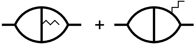
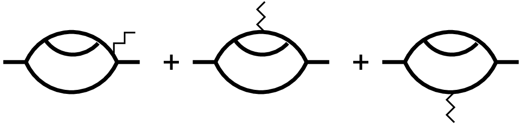
Next, we consider -insertions into the -loop self-energy diagrams. From the diagrams shown in the middle part of Fig. 1, we obtain
| (80) |
Insertions into the -loop self-energy diagrams shown in the lower part of Fig. 1 produce
| (81) |
were , , and are further -independent placeholders stemming from the two apparent choices for taking the replica limit as mentioned above. When we let in the -loop superficially diverging self-energy subdiagram in diagram H before taking the summation over the replicon distribution, we obtain , , and . Otherwise, we get , , and . We will analyze the correct ”timing” of the replica limit in more detail further below.
To calculate the renormalization factors for the fields to -loop order, we collect our various diagrammatic results,
| (82) | ||||
| (83) |
and take the limit . In this limit we obtain
| (84) | ||||
| (85) |
As usual, these renormalization factors, as well as their products have the form of a Laurent series, , etc.
Our ultimate goal is to determine the inverse multifractal dimensions
| (86) |
of the MH model. Thus, we need to extract from the above renormalizations the Wilson function
| (87) |
where is the Gell-Mann–Low function given to 2-loop order in Eq. (41). It follows from Eq. (87) that
| (88) |
has to be free of -poles. Hence, we obtain the t’Hooft-identity [40]
| (89) |
Inserting our -loop results into this identity, we find the condition
| (90) |
This condition has the unique solution and . Thus, to make the Meir-Harris model renormalizable, one necessarily has to take the replica limit in the superficial divergent subdiagram (SDS) appearing in diagram H before one sums over the replicon distributions of H with -insertion. Remarkably, the renormalization factor obtained this way is identical to 2-loop order to the renormalization factor with resulting from the Harris model in conjunction with the real-world interpretation provided that kinetic averaging is used. Consequentially, the same holds true for the multifractal exponents produced by the two approaches. We rate this as a strong indication for the validity of the real-world interpretation with kinetic averaging.
IX Concluding remarks
In summary, we have shown that weak disorder in the SAW-problem is redundant in the sense of the RG for kinetic averaging as it is for static averaging. We have derived the scaling exponents of SAWs in strongly disordered media by field-theoretic methods to second order in the dimensional expansion below six dimensions. We have shown in the real-world interpretation of the corresponding diagrams that in contrast to a static averaging over the SAWs only kinetic averaging lead to a renormalizable theory. The different behavior of these two averaging procedures under renormalization is expected to have important physical consequences for the statistics of polymers in real disordered media. We argue that a statistics of polymers based on static averaging has no asymptotic scaling limit. Based on our findings, we do not expect experiments and numerical simulations using static averaging to produce clear scaling behavior. In fact, we think that the wide-spreading of simulation results for the SAW exponent in strongly disordered media is linked to static averaging.
Closing, we would like to supplement our firm but conceptually somewhat involved field-theoretic argument for the imperative of kinetic averaging by a simple hand-waving argument based on the link-node-blob model of percolation clusters. In this model, the backbone connecting two terminal points of a percolation cluster, which is generically very inhomogeneous and asymmetric, can be envisaged as two nodes linked by a tortuous ribbon that contains blobs. A blob itself is constructed from at least two links joined at two nodes which may again contain blobs. Let us for simplicity consider an asymmetric blob as sketched in Fig. 10 that features two links between two nodes, one with and the other without a blob. Note that this cluster resembles the ominous diagram H of Fig. 1. Assume that the internal blob has many ramifications of short links in it. Hence, say different SAW configurations are possible on the upper link. With static averaging the upper link acquires a much larger weight then the other (lower) one (weight ) even if it may be much shorter than the link without the blob. Then, the statistics of the mean length is dominated by the short upper link with its many different SAWs induced by the blob. However, the weights change drastically upon coarse graining. Suppose we have some coarse graining procedure that culminates in condensing the “microscopic” blob into a single bond. After that, both links have the same weight. However, the lower one, since it is longer, now dominates the statistics. This demonstrates the instability of the weights of static averaging under real space renormalization as the group generated by repeated coarse graining. In contrast, kinetic averaging does assign the same weight to both links independent of the blob. Thus, kinetic averaging is stable under coarse graining even in a strongly asymmetric inhomogeneous disordered medium like the backbone of a percolation cluster. All in all, the behavior of the links-nodes-blobs cluster of Fig. 10 under coarse graining resembles in a nut shell the issues we encountered in our discussion of diagram H of our field theory and thereby corroborates the imperative of kinetic averaging on an intuitive level. Note that real-space RG approaches as employed in Refs. [2, 3] generically use symmetric configurations, and hence static and kinetic averaging lead to equal results in these approaches as they do in ordered media like regular lattices which are trivially homogeneous and symmetric.

Acknowledgements.
This work was supported in part (OS) by NSF-DMR-1104707.Appendix A Dynamical response functional for SAWs in random matter
In this appendix we generalize Peliti’s derivation of a field theory for the statistics kinetically generated SAWs [6]. An excellent review of the method can be find in [42]. To have a starting point, let us revisit the diffusion and reaction processes introduced in Sec. III. First, the rules (9), (10) and (11) for these processes are reformulated in terms of a master equation that describes the time dependence of the probability for a given configuration of site occupation numbers and of the walkers and the markers , respectively. Then, the master equation is transformed in the “second quantisation” formalism developed by Doi [43], Rose [44], and Grassberger and Scheunert [45] as follows. The configuration probability is encoded in the state vector in a bosonic Fock space spanned by the basis . These vectors as well as the stochastic processes in the master equation are expressed through the action of bosonic creation and annihilation operators and , respectively, which are defined via and etc. is the vacuum state without walkers and markers. Subsequently, the master equation can be written in the form
| (91) |
with an appropriate non-Hermitean pseudo-Hamilton operator
| (92) |
Here denotes a pair of neighboring sites. The formal solution of the master equation (91) reads . Suppose we wish to calculate the -walker probability to find the walker at site at time if he starts from site at time not taking into account the resulting distribution of the markers at . Since a walker can be destroyed but not spontaneously generated over the course of time, we have where is the number-operator of walkers at site and where denotes an average whose precise definition will become clear shortly. To compute such a statistical average, it is useful to introduce the projection state . Using the identities and one easily finds
| (93) |
Changing from the occupation-number basis to a Bargmann-Fock space representation with the coherent states (the eigenstates of the annihilation operators) as the basis, and following standard procedures [39, 6, 42] the expectation value (93) can be expressed as a path integral
| (94) |
Here the variables are classical quantities which correspond to the coherent-state eigenvalues, and the functional integral (94) is performed subject to the conditions . The action results from the Hamiltonian (92) as
| (95) |
It is easily seen that the coupling induced by the number in the term of the interaction part of (95) does not contribute to the calculation of the expectation values (Greens functions) , especially to , by perturbational series. Hence we neglect this destroying coupling in the following. Furthermore, the variables and can be integrated out. E.g., performing the functional integral leads to a factor . These -conditions can be easily integrated (remember ) to
| (96) |
The remaining term in which contains yields then
| (97) |
where .
It remains to perform the average of the expectation values over the disorder distribution of the . Note that the normalization factor of the path integral is defined so that , and is purely numeric. Hence, their is no need for the replica trick. The average can be taken directly over . We use a Poissonian disorder distribution
| (98) |
of independent traps on each site , characterized by the mean value . We get
| (99) |
Using this expression, we arrive at a reduced action for the calculation of the disorder averaged Greens functions
| (100) |
As long as the third order terms becomes irrelevant in the RG sense.
To obtain a proper field theoretic functional, it remains to transcribe the formulation from the lattice to the spatial continuum. Performing a naive continuum limit of , several rescalings and a renaming of the variables and parameters, we finally arrive at the dynamical response functional (12).
Appendix B The renormalization of the longest SAW
Here, we present some details of our diagrammatic calculation for the longest SAW. The general formula of the diagrammatic contributions related to the various SAWs we consider in this paper is
| (101) |
where is the set of Schwinger-parameters of a given diagram. is defined through . is a placeholder for the shortest length , the longest length or the average length , respectively, and is a shorthand for the corresponding limit of . Here, we will focus on . The average SAW and the corresponding multifractal moments are treated in the following appendix.
First, let us focus on the 1-loop part of the calculation. For simplicity, we set in the following because we are not interested in reproducing the well-known field-renormalization . Moreover, we will neglect all contributions to diagrams proportional to because we are not interested in reproducing the well-known . At 1-loop order, there are only 2 conducting diagrams, namely diagrams A and B of Fig. (1). These diagrams give
| (102) |
where and where is defined through . Using the renormalization scheme (37), we get the -part of the renormalized selfenergy
| (103) |
It follows the renormalization factor to -loop order:
| (104) |
Now, we turn to -loop order. First, we consider the diagrams C, D, E, F, G. These diagrams lead to the integral
| (105) |
where we have used some invariance under permutations of indices to reduce the number of terms and where we have defined
| (106) |
To simplify the integrations, we introduce new variables,
| (107) |
The integrations over and are cumbersome but manageable and produce after expansion to linear order in
| (108) | ||||
| (109) |
In the same manner we find for the second group of diagrams, H, I, J, K, L,
| (110) |
with
| (111) |
Here, we chose new integration variables
| (112) |
and the integration over and yields
| (113) |
Next we turn to the integration over the -variables. In part, these integrations can be done in an efficient and elegant manner by taking derivatives of the parameter integral
| (114) |
introduced by Breuer and Janssen [46]. The remaining parts can be tackled in the same spirit by introducing a second parameter integral:
| (115) |
In -expansion, we obtain
| (116) |
Via differentiating the parameter integrals with respect to their parameters, we get the -parts
| (117) |
and
| (118) |
Collecting the 1- and 2-loop contributions, we find
| (119) |
for the -part of the renormalized self-energy to order . This form makes evident that non-primitiv divergencies drop out and the -poles are cancelled by choosing
| (120) |
Appendix C Renormalization of the multifractal moments
Now, we present some details of our diagrammatic calculation for the multifractal moments. Our calculation here is based on Eq. (101) with specified to
| (121) |
where is the length of SAW of the bundle of all SAWs on the conducting part of the diagram, its probability, the statistical weight of line of the diagram. More generally, we are interested in all averaged moments of the weights, and hence we consider
| (122) |
with left general. For the - and -loop diagrams to shown in Fig. (1) the probabilities of the SAWs according to the kinetic rule are
| (123) |
Note that only the three SAWs on diagram the kinetic rule lead to different probabilities than the static rule which yields . This fact is discussed in detail in the main text. The statistical weights of the lines of the different diagrams follow from Eq. (121) as
| (124) |
Using these weights as well as the symmetries of the diagrams, we obtain form Eq. (122) the following averaged moments of the weights:
| (125) |
In the following, we replace the control parameter by to emphasize the fact that the multifractal index is kept general in our calculation. Using the substitutions , , the of the -loop self-energy that is linear in becomes
| (126) |
Using the renormalization scheme (37) with the renormalization replaced by
| (127) |
we get
| (128) |
for the -part of the renormalized vertex-function to -loop order. It follows
| (129) |
for the renormalization factors of the .
Now, we turn to -loop order. First, we consider the diagrams C, D, E, F, G. These diagrams lead to the integral
| (130) |
Switching to the integration variables defined in Eq. (107) and integrating over and , the integrals can be expressed once again in terms of the mother-integral . Taking the appropriate derivatives thereof, we obtain
Proceeding similarly, we get for the second group of diagrams H, I, J, K, L
| (131) |
Using the integration variables defined in Eq. (112), we obtain
| (132) |
Collecting the - and -loop contributions, we find
| (133) |
for the -part of the renormalized self-energy to order . It is free of non-primitive divergencies as it should, and the -poles are cancelled by the renormalization factors stated in Eq. (54).
References
- [1] Statistics of Linear Polymers in Disordered Media, edited by B.K. Chakrabarti, (Elsevier, Amsterdam, 2005).
- [2] Y. Meir and A.B. Harris, Phys. Rev. Lett. 63, 2819 (1989).
- [3] C. von Ferber, V. Blavats’ka, R. Folk, and Yu. Holovatch, Phys. Rev. E 70, 035104(R) (2004), and in [1], pg. 103.
- [4] P. Le Doussal and J. Machta, J. Stat. Phys. 64, 541 (1991).
- [5] I. Majid, N. Jan, A. Coniglio, and H.E. Stanley, Phys. Rev. Lett. 52, 1257 (1984).
- [6] L. Peliti, J. Phys. (Paris) Lett. 45, L925 (1984); J. Phys. (Paris) 46, 1469 (1985).
- [7] K. Kremer and J. Lyklema, Phys. Rev. Lett. 55, 2091 (1985).
- [8] L. Pietronero, Phys. Rev. Lett. 55, 2025 (1985).
- [9] A.B. Harris, Z. Phys. B 49, 347 (1983).
- [10] V. Blavatska and W. Janke, Phys. Rev. Lett. 101, 125701 (2008); Physics Procedia 3, 1431 (2010).
- [11] V. Blavatska and W. Janke, Europhys. Lett. 82, 66006 (2008); J. Phys. A 42, 015001 (2009).
- [12] H.K. Janssen and O. Stenull Phys. Rev. E 75, 020801(R) (2007).
- [13] R. Rammal, C. Tannous, and A.-M. S. Tremblay, Phys. Rev. A 31, 2662 (1985); R. Rammal, C. Tannous, P. Brenton, and A.-M. S. Tremblay, Phys. Rev. Lett. 54, 1718 (1985).
- [14] L. de Arcangelis, S. Redner, and A. Coniglio, Phys. Rev. B 31, 4725 (1985).
- [15] Y. Park, A. B. Harris and T. C. Lubensky, Phys. Rev. B 35, 5048 (1987).
- [16] O. Stenull and H.K. Janssen, Europhys. Lett. 51, 539 (2000).
- [17] O. Stenull and H.K. Janssen, Phys. Rev. E 63, 036103 (2001).
- [18] O. Stenull, Renormalized Field Theory of Random Resistor Networks, Ph.D. thesis, Universität Düsseldorf, (Shaker, Aachen, 2000).
- [19] O. Stenull and H.K. Janssen, Phys. Rev. E 65, 036124 (2002).
- [20] H. Hinrichsen, O. Stenull and H.K. Janssen, Phys. Rev. E 65, 045104(R) (2002).
- [21] O. Stenull, H.K. Janssen, and K. Oerding, Phys. Rev. E 59, 4919 (1999).
- [22] O.F. de Alcantara Bonfim, J.E. Kirkham and A.J. McKane, J. Phys. A: Math. Gen. 13, L247 (1980); 14, 2391 (1981).
- [23] H.K. Janssen, O. Stenull, and K. Oerding, Phys. Rev. E 59, R6239 (1999).
- [24] H.K. Janssen and O. Stenull, Phys. Rev. E 61, 4821 (2000).
- [25] S.W. Kenkel and J.P. Straley, Phys. Rev. Lett. 49 , 767 (1982); J.P. Straley and S.W. Kenkel, Phys. Rev. B 29, 6299 (1984).
- [26] R. Blumenfeld and A. Aharony, J. Phys. A 18, L443 (1985); R. Blumenfeld, Y. Meir, A.B. Harris and A. Aharony, J. Phys. A 19, L791 (1986).
- [27] A.B. Harris, Phys. Rev. B 35, 5056 (1987).
- [28] M.J. Stephen, Phys. Rev. B 17, 4444 (1978).
- [29] This step also helps to avoid factors like . When interpreted properly, i.e., when is interpreted as the limit of a finite quantity and the replica limit is taken at first these factors reduce to unity and are hence harmless. Nevertheless, avoiding these factors helps to keep calculations clutter free.
- [30] A.B. Harris and T.C. Lubensky, J. Phys. A 17, L609 (1984), Phys. Rev. B 35, 6964 (1987).
- [31] J. Wang, J. Phys. A 22, 219 (1989).
- [32] H.K. Janssen and O. Stenull, Phys. Rev. E 69, 026118 (2004).
- [33] O. Stenull and H.K. Janssen, Europhys. Lett. 51 , 539 (2000); Phys. Rev. E 63, 036103 (2001).
- [34] H.K. Janssen, Z. Phys B: Condens. Matter 58, 311 (1985).
- [35] H.K. Janssen and O. Stenull, to be published.
- [36] Note that in the figure shown in reference [3] a factor of the second order term is missed.
- [37] A.B. Harris and T.C. Lubensky, Phys. Rev. B 35, 6987 (1987).
- [38] A.B. Harris, Phys. Rev. B 28, 2614 (1983).
- [39] C. Itzykson and J.-B. Zuber, Quantum Field Theory (McGraw-Hill, New York, 1980).
- [40] G. t’Hooft, Nucl. Phys. B 61, 455 (1973).
- [41] J.D. Bjorken and S.D. Drell, Relativistic Quantum Fields (McGraw-Hill, New York, 1965).
- [42] U.C. Täuber, M. Howard, and B.P. Vollmayr-Lee, J. Phys. A 38, R79 (2005).
- [43] M. Doi, J. Phys. A 9, 1465, 1479 (1976).
- [44] H.A. Rose, J. Stat. Phys. 20, 415 (1979).
- [45] P. Grassberger and M. Scheunert, Fortschr. Phys. 28, 547 (1980).
- [46] N. Breuer and H.K. Janssen, Z. Phys. B 41, 55 (1981).