Slopes of Kantorovich potentials and existence of optimal transport
maps in
metric measure spaces
Abstract.
We study optimal transportation with the quadratic cost function in geodesic metric spaces satisfying suitable non-branching assumptions. We introduce and study the notions of slope along curves and along geodesics and we apply the latter to prove suitable generalizations of Brenier’s theorem of existence of optimal maps.
Key words and phrases:
Optimal transportation, geodesic metric space, non-branching, upper gradient2000 Mathematics Subject Classification
Primary 49Q20, 53C23.1. Introduction
The problem of finding an optimal way to transport mass has a long history, starting from Monge’s seminal paper [14]. The optimality of a transport can be measured in many ways, depending on the choice of the cost function. In this paper we focus on the case when the cost is the square of the distance.
Given two positive and finite measures and on some metric space with the same total mass, which we may normalize to 1, our task is then to study whether the infimum
| (1.1) |
over all possible -measurable maps which send the measure to , is attained. If such a minimizing map exists, we call it an optimal transport map between and . Existence of optimal maps or even of admissible ones is problematic, for instance no admissible map exists when is a Dirac mass and is not a Dirac mass.
Kantorovich’s relaxed [9, 10] formulation of the optimal transport problem consists in finding the infimum
| (1.2) |
over all possible transport plans, i.e. probability measures on which have and as marginals. Again, if there is a measure which attains the infimum, it is called an optimal transport plan between and . Notice that transport plans can split measure, and so they avoid the problem faced by transport maps. In fact, not only the Kantorovich formulation of the problem is well-posed, but the infimum is attained (possibly infinite) under the only assumption that is complete and separable. Since we will be dealing with geodesic metric spaces, we will mostly work with the equivalent formulation in terms of geodesic transport plans, i.e. probability measures in the space of constant speed geodesics parameterized on , with marginal conditions at and .
In general, it seems to be a difficult problem to find necessary and sufficient conditions under which Monge’s problem has a solution, but by now several sufficient conditions are known. For the quadratic cost in the Euclidean setting it was proved independently by Brenier [6] and Smith and Knott [16] that there exists a unique optimal map , given by the gradient of a convex function, provided that is absolutely continuous with respect to the Lebesgue measure. This result was generalized to Riemannian manifolds by McCann [13], to Alexandrov spaces by Bertrand [5] to the Heisenberg group by Ambrosio and Rigot [4] and, very recently, to non-branching metric spaces with Ricci curvature bounded from below (in the sense of Lott, Sturm and Villani) by Gigli [8]. Notice that in all these results a reference measure (Lebesgue measure, Riemannian volume, Haar measure, etc.) plays a role, so the proper setting for this question is the family of metric measure spaces .
In another recent paper [1], a metric Brenier theorem is proved under mild assumptions on , see Theorem 10.3 and Remark 10.7 therein. In the case when has bounded diameter and is a finite measure, the main assumption is the existence of bounds on the relative entropy along geodesics (a condition weaker than the condition of Lott, Sturm and Villani) and the metric Brenier theorem states that, for any optimal geodesic plans , it holds
| (1.3) |
(here is any Kantorovich potential and is its ascending slope). In other words, the transportation distance depends -a.e. only on the initial point.
This result raises some questions that we plan to investigate in this paper: the first one is to understand under which additional assumptions one can really recover an optimal map, the second one is about the differentiability of along geodesics used by the optimal plan.
In connection with the first question we start from this heuristic idea more or less implicit in many proofs: under appropriate structural assumptions on the space, (1.3) identifies the “initial velocity” of the geodesic. Indeed, assuming suitable non-branching assumptions on the space and on its tangent metric spaces we can perform a suitable blow-up analysis that leads to the existence of optimal maps. The proof of this result requires a detailed analysis of the proof of the metric Brenier theorem in [1] and the introduction of a sharper notion of ascending slope, namely the ascending slope along geodesics. Since we believe that this concept has an independent interest we compare this slope to the usual one and to the slope along curves, we provide an example and we raise some open problems. Coming back to the existence of optimal maps, our result covers as a particular case the Euclidean, the Riemannian and the Alexandrov case, see also the paragraph immediately after Theorem 4.3 for a more detailed discussion.
In connection with the second question, it has already been proved in Theorem 10.4 of [1] a “differentiability in mean”, namely
| (1.4) |
This weak differentiability property plays an important role in the subsequent paper [2], for the computation of the derivative of the entropy along geodesics. Here, under an additional doubling assumption on , we are able to improve (1.4) to a pointwise differentiability property, so that
for -a.e. .
Acknowledgement. The authors acknowledge the support of the ERC ADG GeMeThNES. The second author also acknowledges the support of the Academy of Finland, project no. 137528.
2. Non-branching metric spaces
Let us start by laying out the definitions for the metric spaces that will be used in this paper. First of all, we will be working exclusively in metric spaces which are complete and separable. Second, by measure in we mean a nonnegative Borel measure, finite on bounded sets. We will mainly consider metric spaces equipped with a doubling measure meaning that there exists a constant so that for all and we have
A related notion for metric spaces where the measure has not been specified is that of a doubling metric space, which means that there exists an integer so that, for all , any ball of radius can be covered by balls of radius . It is obvious that if there exists a doubling measure on then the space has to be doubling as well. The converse is also true for complete metric space, see for example [12] and [11].
We call any absolutely continuous map a curve and use the abbreviation . The length of the curve is defined as
We call the curve a geodesic if . The metric space itself is called geodesic if any two points can be connected with a geodesic, i.e. there exists a geodesic with and . Sometimes, when there is no danger of confusion, we also call the image of a geodesic a geodesic.
The speed of a curve is given by
whenever the limit exists. It is not hard to prove, see for instance Theorem 1.1.2 in [3], that it indeed exists at -almost every point , where is the Lebesgue measure on , and that .
We denote by the set of all constant speed geodesics in which are parametrized by , namely for all . By a reparameterization argument, constant speed geodesics connecting any two given points exist in any geodesic space. We equip the space with the distance
and note that is also complete and separable since the underlying metric space is. We will also use the convenient notation of evaluation map , defined as for all .
With the basic notation related to geodesics now fixed we are ready to introduce the two definitions of non-branching which play a crucial role in our results.
Definition 2.1.
We call a geodesic metric space non-branching if for any two constant speed geodesics with and for some we have for all .
We would like to use non-branching on the level of the tangent spaces. However, two distinct geodesics of a metric space can collapse into a single geodesic of the tangent space in the blow-up. To control such collapsing we will assume a stronger version of non-branching.
Definition 2.2.
We call a geodesic metric space strongly non-branching if for any two constant speed geodesics with , and , we have
| (2.1) |
In our main theorem, Theorem 4.3, we assume that the space is strongly non-branching and that at almost every point we have some non-branching tangent space. Before defining what we mean by tangent space we recall the definitions of Hausdorff- and Gromov-Hausdorff-distance. The Hausdorff-distance between closed sets is defined as
Using the Hausdorff-distance, the Gromov-Hausdorff-distance between two metric spaces and is then defined as
where the infimum is taken over all metric spaces and isometries , . Finally, a sequence of metric spaces and points is said to converge to in the pointed Gromov-Hausdorff sense if
where by we denote the closed ball. Given a metric space and a scaling factor , we define a rescaled metric on by setting
for all .
Definition 2.3.
Let be a metric space. We call a metric space tangent to at if there exist a sequence and so that
in the pointed Gromov-Hausdorff convergence.
Notice that our definition of a tangent space is weaker than Gromov’s original notion. He required the tangent space to be the full limit of the spaces as , whereas in our definition we only require convergence along a subsequence. As a consequence, with our definition the space can in principle have a huge collection of different tangent spaces at a single point.
We will use the following well-known result (see for instance [2, Proposition 2.7]) which allows us to move from the Gromov-Hausdorff convergence to Hausdorff-convergence.
Theorem 2.4.
If in the Gromov-Hausdorff convergence then there exist a space and isometric embeddings
so that in the Hausdorff convergence.
In addition, if are equi-compact, then
can be taken to be a compact metric space.
3. Gradients along geodesics
Let us recall some basic definitions in measure theory. The collection of universally measurable sets of the space , denoted by , is the -algebra of the sets which are -measurable for all finite nonnegative Borel measure of . The collection of all Borel sets of will be denoted by .
Now we turn to our next set of definitions that concern metric differentials.
Definition 3.1.
Given a function we define the lower ascending slope along geodesics of at as
where + denotes the positive part and the supremum is taken over all nonconstant geodesics in that start from the point .
Here ascending refers to the fact that we are taking the positive part of the difference quotient and lower refers to the fact that we are taking the , rather than the .
Proposition 3.2.
Suppose that is continuous. Then is universally measurable.
Proof.
Let and consider the sublevel set . For the universal measurability it is sufficient to show that this set is Suslin. Because is complete and separable, so are and . Therefore , being the projection of the set
to the space , is indeed Suslin since the projected set can be written as
and so it is Borel (countable intersection of countable unions of open sets). ∎
Definition 3.3.
A function is an upper gradient along geodesics of a function if for any we have
| (3.1) |
where the integral along is understood as
The almost everywhere differentiability of Lipschitz functions on the real line implies that ascending slopes are upper gradients for Lipschitz functions. We include the easy proof of this fact here for the convenience of the reader. Recall that a function is called Lipschitz if there exists a constant so that for any two points we have
Proposition 3.4.
Let be Lipschitz. Then the lower ascending slope along geodesics is an upper gradient along geodesics.
Proof.
By Proposition 3.2 the function is universally measurable, and it is easily seen that this implies the -measurability of (just consider the push forward under of ), see also [1, Lemma 2.4]. Take . The function is Lipschitz and therefore differentiable -almost everywhere. In particular, holds and both sides of the inequality are well defined at -almost every point . Thus
∎
It is interesting to compare the ascending slope and the upper gradient defined along geodesics to the more commonly used versions. First of all, it is immediate that we always have
| (3.2) |
where the usual ascending slope of at a point is defined as
and the lower ascending slope along curves as
with the supremum taken over all curves (recall that by convention all curves we consider are absolutely continuous). Moreover, the inequalities in (3.2) can be strict. Notice also that the choice of the lower concept (i.e. with the ) is justifed by the fact that the upper concept is easily seen to coincide with ).
Recall that we have the usual notion of an upper gradient of a function if we require the inequality (3.1) to hold along all curves on , where this time is understood as . It is not difficult to show, following the same proof given in Proposition 3.2, that ascending slopes along curves are universally measurable. Moreover, as in Proposition 3.4, one can prove that ascending slopes along curves are upper gradients for Lipschitz functions.
Ascending slopes along geodesics could be thought, identifying geodesics to the tangent space as in the theory of Alexandrov spaces, as directional one-sided derivatives. Hence, it is natural to ask if ascending slopes along geodesics are also upper gradients (in the usual sense) for Lipschitz functions. This is not true in general, as we will see in the next example.
Example 3.5.
There exist a separable complete geodesic metric space and a Lipschitz function so that is not an upper gradient of .
Let us first construct the metric space . We start the construction by taking a unit line-segment, which we simply denote by . Next for all and we connect the points and in with an arc of length . In Figure 1 the arcs are drawn as half-circles. The space is then the disjoint union of the arcs and the initial line-segment .
We define the distance between two points as
where the infimum is taken over all collections of ’s that connect the points and , are subsets of the arcs and is the length of the piece determined by the length of the arc. This way on each arc the distance is given by the natural distance determined by the length of the arc. See the left part of Figure 1 for an illustration of the space.
Let us check that is geodesic. Let be two distinct points. If it happens that and lie on the same arc then the segment of the arc joining the points is our geodesic. We may then assume that the points are not on the same arc. We may also assume that . If this is not the case, for example , we simply notice that any curve connecting the points and must go via one of the end-points and of the arc in which lies in and that
We can now find the geodesic between the points and with the following procedure. Let be a sequence of curves joining to so that . Because the lengths of the arcs are chosen so that the shortest curve between points and is the arc , there exists so that each , , contains some with
| (3.3) |
and with some . So, taking a subsequence of we may assume that all the curves contain the same arc . Continuing inductively in the same way with the end-points of this arc and the points and , and finally using a diagonal argument, we obtain the geodesic.
We define the Lipschitz function first on by setting . This fixes the function on the end-points of all the arcs. We continue it inside the arcs by defining for all and
where is the constant speed geodesic joining to in . See the right part of Figure 1 for the graph of the function along a couple of the arcs and the line .
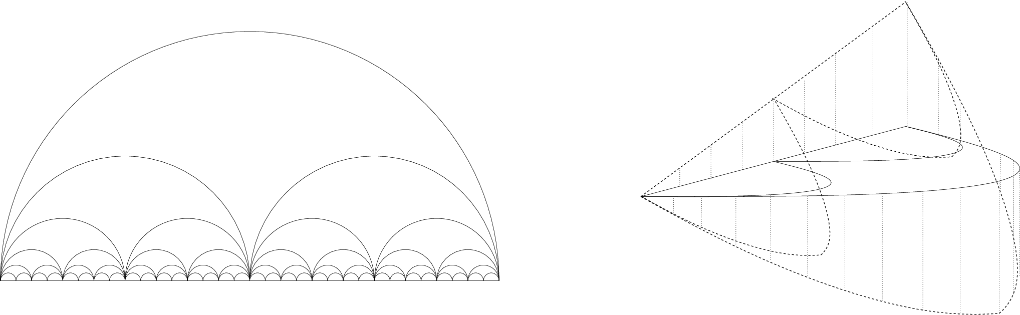
Let us now show that for all . To see this take a geodesic starting from a point . If near the point consists only of one piece of an arc the equality
is immediate. Suppose then that for every there exists a point which is in the considered geodesic and . As we have noted before, the part of that connects to must contain an arc with bounded as in (3.3) and with some . Moreover, we can take such an that . Let be the middle point of . Now , and so indeed .
On the other hand, the constant speed curve has length and is therefore an admissible test curve for the upper gradient property.
It is easy to see that the space in our previous example is not doubling and that it is extremely branching. In light of the example one could still hope many natural conjectures to be true.
Question 3.6.
Which assumptions are needed on the metric space and on the measure to ensure for any Lipschitz function that
- (i)
the equality holds at -almost every point ?
- (ii)
the function is an upper gradient of ?
Notice that if we assume that if is a doubling measure on then -a.e. in (see [1, Proposition 2.5] for the simple proof of this fact) for any Lipschitz function .
In addition, if supports a -Poincaré inequality, then we can apply Cheeger’s theory to obtain -a.e. in for any (weak) upper gradient of . Choosing yields
For the same reason, under the same doubling and Poincaré assumptions, a positive answer to question (ii) implies a positive answer to question (i): indeed, choosing one obtains
4. Mass transportation in metric spaces
Before stating and proving our main results we briefly discuss in the next subsection the basic properties of transport plans and maps in the general metric space setting. A comprehensive treatment of the theory can be found for example in [3] and [17].
4.1. Basic properties of transport plans
Let denote the set of all Borel probability measures on . The Wasserstein distance between two measures is defined as
| (4.1) |
where the infimum is taken over all transport plans between and , i.e. measures for which and . Here the mappings and denote the projections to the first and second coordinate respectively. The notation for a measure and a -measurable mapping means the push-forward measure defined as for all . Notice that in general might be infinite. We call a transport plan between two measures , for which , optimal if the infimum in (4.1) is attained at .
Since we are dealing with geodesic spaces, we can equivalently consider geodesic transport plans. We define the set of geodesic plans between and as the set of all for which , . We say that a geodesic plan is optimal, and write , if
Given an optimal geodesic plan , it is clear that is an optimal plan. Conversely, making a measurable selection of constant speed geodesics from to and considering the law of under , any optimal plan can be “lifted” to an optimal geodesic plan with the same cost.
The Kantorovich formulation of the transportation problem has also a very useful dual formulation: The minimum in (1.2) is equal to
where the supremum is taken among all pairs satisfying .
We define the -transform of a function as
A function is called -concave if for some function . This terminology (-transform, -concavity) refers to a general cost function . Here and in the sequel the cost function is given by the halved square of the distance.
Definition 4.1.
Given an optimal geodesic plan we call a Borel function a Kantorovich potential (relative to the optimal geodesic plan ) if it is -concave and
Notice that because the Kantorovich potential is -concave we have and that we make no integrability assumption on and .
A set is called cyclically monotone if
for any and permutation of .
Suppose that and . Then is supported on a cyclically monotone set and a Kantorovich potential relative to exists.
4.2. Brenier theorem in metric spaces
As a starting point we prove the following result which originates from [1, Theorem 10.3]. The difference compared to the original result is in the definition of the ascending slope, here replaced by the lower ascending slope. Also, we like to repeat the proof in our situation for the convenience of the reader.
Proposition 4.2.
Suppose that is a finite measure on a bounded space and , . Take and let be a Kantorovich potential relative to . If there exists satisfying for all and
| (4.2) |
then
Proof.
By the definition of the Kantorovich potential we have
| (4.3) |
for -a.e. . On the other hand, for any we have
| (4.4) |
Thus combining these two we get that for -a.e. it holds
Let us now prove the converse inequality in an integral form. Taking in (4.4) and combining it with (4.3) we obtain
| (4.5) |
Because is bounded, is Lipschitz and so by Proposition 3.4 the function is an upper gradient of along geodesics. Thus we have
Dividing this by and integrating over yields
From the assumption (4.2) we know that
Because is finite and is bounded, this holds also for . Therefore
∎
With the help of the Proposition 4.2 we are now able to prove a Brenier-type theorem in strongly non-branching metric spaces.
Theorem 4.3.
Assume that is a strongly non-branching geodesic metric space equipped with a doubling measure , and that , satisfy . Assume also that:
- (a)
for -almost every point the space has a non-branching tangent at ;
- (b)
there exists a transport plan such that for all sufficiently small we have and the densities satisfy
Then the optimal geodesic plan is given by a mapping , i.e. for -a.e. .
Proof.
Suppose that there is no such . If we then fix a point and consider the restricted and rescaled measures
we notice that for large enough the assumptions of the theorem are satisfied and still there exists no such . Therefore we may assume the space to be bounded.
Let be the Kantorovich potential relative to . Let be a point where the space has a non-branching tangent. Suppose that there are two geodesics so that ,
| (4.6) |
and
Let be a non-branching geodesic metric space tangent to at and a sequence so that
in the pointed Gromov-Hausdorff convergence as . Since we assumed to be doubling, the spaces are easily seen to be equi-compact. Indeed, for any we can find a maximal disjoint family of balls of radius contained in , so that the family of balls with doubled radius covers , and use the doubling inequality
(here and depend on the doubling constant only) with and to estimate the number of these balls with a constant depending only on , and . We can then apply Theorem 2.4 to obtain a compact space and isometric embeddings
so that in the Hausdorff convergence.
From (4.6) we get for every a constant speed geodesic with and a radius so that
for every for which .
Now, possibly taking a subsequence of so that , we get a sequence of points with and
| (4.7) |
Notice also that for any we have
| (4.8) |
Writing for the for which , triangle inequality and geodesic property yield
| (4.9) |
Hence, using first (4.9), then (4.8) and eventually (4.7) we have
By taking a subsequence we find points so that
In particular
and so lies on some constant speed geodesic in joining to (obtained by the concatenation of the geodesics joining to and to ).
With a similar argument we can show that lies on some constant speed geodesic in joining to , where is obtained as the limit of the points which are taken from the geodesic so that . Note that we might have to go to yet another subsequence to achieve the convergence to .
Because the space is strongly non-branching we have
and so the geodesics and contradict the assumption that is non-branching.
This means that our assumptions on the geodesics and can not be satisfied. Therefore there exists a set so that and for every there is at most one with . Using the set we can define the transport map as
∎
Remark 4.4.
One could prove Theorem 4.3 also under slightly different assumptions. Namely by weakening the definition of strongly non-branching metric space by replacing the liminf in (2.1) to limsup, and then assuming that at almost every point all the tangent spaces to are non-branching. This modified theorem is achieved by letting the sequence of radii in the blow-up be dictated by the weakened form of strong non-branching property, namely choosing in such a way that and .
Theorem 4.3 applies, for example, when the space is a finite dimensional Alexandrov space and is the corresponding volume measure on . The estimate (4.2) on the relative entropy follows in this case from the result of Petrunin [15] which shows that in Alexandrov spaces the functional
| (4.10) |
is concave along Wasserstein geodesics. Notice that a different proof for the Brenier theorem in Alexandrov spaces was already given by Bertrand in [5].
Brenier theorem has been recently established by Gigli [8] in non-branching spaces with Ricci-curvature bounded from below. This generalizes the previous result by Bertrand and it covers for example the case where the functional (4.10) is concave along geodesics in the Wasserstein space of a non-branching space . Whereas our proof of Theorem 4.3 is based on the behaviour of blow-ups and the Kantorovich potential, the proof by Gigli relies on the concavity of the functional and does not use the Kantorovich potential at all. Notice that because of the different techniques used in the proofs our geometric assumptions on the metric space differ from those assumed by Gigli and hence the two theorems cover different collection of metric spaces.
It is also important to notice that our Theorem 4.3 by no means covers all the cases where the Brenier theorem is known to hold. For example the Brenier theorem holds in the Heisenberg group [4], but it is not difficult to see that the Heisenberg group is not strongly non-branching.
We end this paper with an improvement of [1, Theorem 10.4.] in the case where the reference measure is doubling. In [1] it was shown that without the assumption that is doubling we have the conclusion
in the following theorem. Because our Proposition 4.2 was proved in the case where the space is bounded, we will make the same boundedness assumption here. As in many of the results in [1] we could remove this assumption by requiring the density of the initial measure with respect to to be uniformly bounded away from zero.
Theorem 4.5.
Let be a doubling measure on a bounded metric space and , with -a.e. in and . Let and be a Kantorovich potential relative to satisfying
| (4.11) |
Further assume that there exists such that for all we have . Then for -a.e. we have
Proof.
If the lower ascending slope along geodesics of the Kantorovich potential were continuous, the theorem would follow immediately from the fact that the lower ascending slope is an upper gradient. This is not true in general, but what we can prove using density points and cyclical monotonicity is that for -almost every geodesic the lower ascending slope is continuous along the geodesic at its starting point.
On the other hand, by Proposition 3.4 we know that is an upper gradient of along geodesics and so for all the estimate
holds for all . So, our claim follows if we can show with any that for -a.e.
| (4.12) |
when (depending on and ) is small enough.
Because , we know from (4.11) that for -a.e. there exists with and . When we combine this with the assumption , for any , we get for -a.e. a curve so that and
Hence, by Fubini’s theorem we know that for -a.e. a curve with the above properties exists for -a.e. .
Our task is now to estimate from above. Because is doubling, it is enough to prove this for for which is a Lebesgue point of . Let and take so small that for every and , where , there exists with and
| (4.13) |
Define and let . With this choice of let be as above. Notice that we may assume , as otherwise the upper bound on immediately follows. The selected curves are illustrated in Figure 2.

References
- [1] L. Ambrosio, N. Gigli and G. Savaré, Calculus and heat flow in metric measure spaces and applications to spaces with Ricci bounds from below, preprint, 2011.
- [2] L. Ambrosio, N. Gigli and G. Savaré, Metric measure spaces with Riemannian Ricci curvature bounded from below, preprint, 2011.
- [3] L. Ambrosio, N. Gigli and G. Savaré, Gradient flows in metric spaces and in the space of probability measures, Lectures in Mathematics ETH Zürich, Birkhäuser Verlag, Basel, second ed., 2008.
- [4] L. Ambrosio and S. Rigot. Optimal mass transportation in the Heisenberg group, J. Funct. Anal., 208 (2004), no. 2, 261–301.
- [5] J. Bertrand, Existence and uniqueness of optimal maps on Alexandrov spaces, Adv. Math., 219 (2008), no. 3, 838–851.
- [6] Y. Brenier, Polar factorization and monotone rearrangement of vector valued functions, Comm. Pure and Appl. Math., 64 (1991), 375–417.
- [7] J. Cheeger, Differentiability of Lipschitz functions on metric measure spaces, GAFA, 9 (1999), 428–517.
- [8] N. Gigli, Optimal maps in non branching spaces with Ricci curvature bounded from below, preprint, 2011.
- [9] L. V. Kantorovich, On the translocation of masses, C.R. (Dokl.) Acad. Sci. URSS, 37 (1942), 199–201.
- [10] L. V. Kantorovich, On a problem of Monge (in Russian), Uspekhi Mat. Nauk. 3 (1948), 225–226.
- [11] A. Käenmäki, T. Rajala and V. Suomala, Existence of doubling measures via generalised nested cubes, Proc. Amer. Math. Soc., to appear.
- [12] J. Luukkainen and E. Saksman, Every complete doubling metric space carries a doubling measure, Proc. Amer. Math. Soc., 126 (1998), no. 2, 531–534.
- [13] R. McCann, Polar factorization of maps on Riemannian manifolds, Geom. Funct. Anal., 11 (2001), 589–608.
- [14] G. Monge, Mémoire sur la théorie des déblais et remblais, Mémoire de l’académie des sciences de Paris, 1781.
- [15] A. Petrunin, Alexandrov meets Lott-Villani-Sturm, Münster J. of Math., to appear.
- [16] C. Smith and M. Knott, On the optimal transportation of distributions, J. Optim. Theory Appl., 52 (1987), 323–329.
- [17] C. Villani, Optimal transport. Old and new, vol. 338 of Grundlehren der Mathematischen Wissenschaften, Springer-Verlag, Berlin, 2009.