Measurement-Based Quantum Computing with Valence-Bond-Solids
Abstract
Measurement-based quantum computing (MBQC) is a model of quantum computing that proceeds by sequential measurements of individual spins in an entangled resource state. However, it remains a challenge to produce efficiently such resource states. Would it be possible to generate these states by simply cooling a quantum many-body system to its ground state? Cluster states, the canonical resource states for MBQC, do not occur naturally as unique ground states of physical systems. This inherent hurdle has led to a significant effort to identify alternative resource states that appear as ground states in spin lattices. Recently, some interesting candidates have been identified with various valence-bond-solid (VBS) states. In this review, we provide a pedagogical introduction to recent progress regarding MBQC with VBS states as possible resource states. This study has led to an interesting interdisciplinary research area at the interface of quantum information science and condensed matter physics.
1 Introduction
Although Richard Feynman [1] mooted the idea of a quantum computer nearly thirty years ago in 1982, serious research work into quantum computing probably only appeared about fifteen years ago when Peter Shor demonstrated that a quantum computer, if available, could perform prime number factorization exponentially faster than a conventional computer which we typically call "classical computer". A quantum computer essentially exploits inherently quantum mechanical properties like the linear superposition principle and entanglement to improve computational speed and complexity.
In Feynman’s original idea, a quantum computer, if constructed, would be also an ideal machine for simulating naturally-occurring many-body quantum problems. After all, nature is largely quantum mechanical and the ideal platform for solving problems in nature should be a quantum mechanical device. From a theoretical computer science perspective, the rigorous foundation of a quantum computing device was laid, in 1985, by David Deutsch at Oxford who cleverly formulated a theoretical model called the quantum Turing machine [2], which has been a fundamental lego block for the study of a quantum computer.
In 1989, Deutsch introduced another model of fundamental importance for quantum computation: the quantum circuit model [3]. Yao then showed in 1993 that the circuit model is actually equivalent to the quantum Turing machine in terms of their computational power [4]. As we have mentioned before, Shor published his famous algorithm for efficient prime numbers factorization on a quantum computer in 1994 [5]. Factoring is believed to be a difficult problem to solve on a classical computer and it lies at the heart of modern cryptographic technology: the Rivest-Shamir-Adleman (RSA) scheme. Shor’s theoretical insight, if realized, thus poses an immediate threat to classical cryptographic security. Equipped with quantum computers, all security systems currently in use based on the computational difficulty of large prime number factorization would be rendered useless.
The basic entity in classical computing is the bit. A bit is usually encoded in several ways, for instance, the voltage or current in a wire or the energy in a capacitor. In a quantum computer, the information can also be encoded in different ways: for instance, the polarization of a photon or the energy levels of a two-level atomic or molecular system. Unlike classical bit, the information for a two-level quantum system can be encoded in a superposition of the two levels of the system. Such encoding is called a quantum bit or a qubit. Thus, qubits form the basic building blocks for a quantum computer.
Classical computation proceeds essentially through a series of wires and gates. The quantum circuit model in which algorithms are implemented through a series of quantum gates thus remains the most promising paradigm for the large scale realization of a quantum computer. For a quantum computer, the circuit model applies a sequence of unitary operations on an initial quantum state of a system with qubits and evolves the quantum system according to the Schroedinger equation. Although each single gate usually acts non-trivially on only one or two qubits, the concatenation of these gates proves to be sufficient for producing any unitary operation on the -qubit initial state , a property known as “universal” computation. The application of this sequence of gates transforms an initial state into a final state . The final computational result is then extracted from appropriate measurements on the final state.
The realization of the quantum circuit model in various physical systems has been extensively studied. These approaches include implementation through nuclear magnetic resonance [6], the manipulations of atoms or ions in ion traps [7], the manipulation of neutral atom [8], implementation with cavity QED [9], the optical platform with linear or nonlinear optical devices [10], manipulation of electrons or atoms in the solid state [11], superconducting devices [12], and a “unique” qubit scheme [13]. Regardless of the approach in the realization of large scale quantum computing, DiVincenzo has elegantly summarized five important criteria for the physical implementation of future quantum computers [14], and each one of these criteria has been carefully examined [7, 8, 9, 10, 11, 12, 13, 14]. To date none of these systems is capable of realizing a large scale quantum computer in the foreseeable future without any glitches: each system presents uniquely its own set of challenges and problems. And indeed one important stumbling block is that many quantum gates entangling two qubits cannot be implemented with high fidelity in many of these systems [15]. To overcome some of these limitations, researchers have sought other paradigms of quantum computation. Although these alternative paradigms are equivalent to the quantum circuit model in terms of computational power, they are very different in terms of real physical realization. Among these other paradigms, some of more promising ones are measurement-based quantum computing [16], topological quantum computing [17] and adiabatic quantum computing [18].
In this review, we focus on the measurement-based quantum computing (MBQC) model, first introduced by Raussendorf and Briegel in 2001 [16]. MBQC is a model of quantum computing that is equivalent to the circuit model in terms of computational power, given that it can simulate every single-qubit gate and two-qubit gate in the circuit model in an efficient way, and it is thus universal for quantum computing. However, the physical realization of MBQC is very different from that of the circuit model. It starts from a highly entangled multi-qubit state , called a cluster state. Sequential single-qubit measurements are then performed on the cluster state to realize quantum computing. The advantage of MBQC is that once is prepared, no entangling gates are needed in process of the computation. Or one may imagine that all the entanglement needed for a quantum computation is already embodied in . MBQC thus seems very appealing for the implementation of quantum computing provided that can be efficiently prepared initially and maintained during the process of measurements.
Perhaps the most natural and simplest means of preparing an entangled quantum state is to search for a many-body system in which the unique ground state is the required entangled resource. With correct cooling techniques, one should then be able to acquire the ground state and hence the entangled resource state needed for MBQC. Unfortunately, it turns out that does not naturally occur as unique ground states of any naturally-occurring physical systems. More precisely, it was shown by Nielsen that cannot even be a unique ground state of any Hamiltonian of qubits involving at most two-particle interactions [19]. It is then highly desirable seeking for other many-body quantum states, with which MBQC can be performed in a similar manner as is performed on , where only single-particle measurements are needed to implement universal quantum computing. We call these alternative states for MBQC “resource states”. Moreover, we want these resource states to naturally occur as unique ground states of some lattice spin systems, that is, unique ground states of Hamiltonians involving only two-particle nearest-neighbor interactions on a lattice. In addition, one also wants the resource states to be stable during the process of measurements, that is, to remain as a ground state of the Hamiltonian after the particles are measured and discarded. To satisfy this condition, it is sufficient that the Hamiltonian is “frustration-free”, that is, the ground state of the Hamiltonian is also a ground state of each interaction term of the Hamiltonian. Another desired property is that the Hamiltonian is gapped, meaning that it has a constant energy gap regardless of the system size (i.e., the number of particles), so the ground state can be stable against thermal fluctuation.
In 2007, Gross and Eisert took the first step towards the construction of such realistic resource states for MBQC [20]. They introduced an interesting framework for producing resource states which is closely related to the theoretical description of valence-bond-solids (VBS). The gist of their proposal is that even if the quantum computation is actually performed on a system of qubits, the actual physical system is not just a system of particles with information encoded in two different levels. These particles could ideally possess higher spins - a feature which greatly facilitates the search for realistic lattice Hamiltonians. Their framework allows one to construct various resource states with different spin values and on different types of lattices. For resource states associated with realistic Hamiltonians, they found Hamiltonians on a spin- chain, involving only nearest-neighbor interactions, whose unique ground states are resource states for MBQC. Moreover, these systems are also frustration-free and gapped. Unfortunately, their scheme applies specifically to one-dimensional(1D) spin chains. Since a 1D spin chain can only process quantum computation of a single qubit, their framework are not universal. It was also not obvious how one could extend the scheme to find any realistic two-dimensional(2D) resource states for MBQC. In 2008, Brennen and Miyake showed that a famous one-dimensional VBS state, the Affleck-Kennedy-Lieb-Tasaki (AKLT) state on a spin- chain [21] with certain boundary condition, can act as a resource state for MBQC [22]. Although this is still a result for 1D chain, it sharpens the connection between the studies of MBQC and VBS states [23].
In 2009, Chen et al. took an important step towards the construction of 2D realistic resource states for MBQC [24]. They showed that a state of a spin- system on the honeycomb lattice, called the tri-Cluster state, is a unique ground state of a frustration-free, gapped, two-body Hamiltonian with only nearest-neighbor interactions. Although the form of the actual spin Hamiltonian appears complicated, their method does open up new possibilities for constructing other 2D realistic resource states for MBQC. In early 2010, Cai et al. then constructed a realistic resource state of a spin- system on the 2D octagonal lattice, called a quantum magnet, which is in turn based on proper coupling of spin- quasi-AKLT chains. In the same year, Chen et al. developed an interesting alternative viewpoint on the universality of VBS states for MBQC, by showing that these known resource states can be reduced to the cluster states via adaptive local measurements at a constant cost [25]. This viewpoint turns out to be particularly useful for studying the universality of VBS states for MBQC, as cluster states themselves can be viewed as VBS states that was first realized by Verstraete and Cirac in 2004 [26]. Also based on this viewpoint, Wei et al. reinterpreted the universality of the quantum magnet by reducing this resource states to a 2D cluster state [27]. Interestingly, Wei et al. and Miyake independently discovered that the 2D AKLT state on the honeycomb lattice can also be a resource state for MBQC [28, 29, 30]. Although it is still unclear if the 2D AKLT Hamiltonian on the honeycomb lattice is gapped [31], this result nicely links the study of MBQC and VBS.
The “quick reduction” from spin- to spin- systems for realistic 2D resource states for MBQC naturally gave further impetus for the search of realistic resource states in a spin- system. Unfortunately, it was recently shown by Chen et al. that this may not be possible. Chen et al. provided a no-go theorem showing that there does not exist a unique ground state for a two-body frustration-free Hamiltonian that can simultaneously be a resource state for MBQC [32] for a qubit system. It was further shown by Ji et al. that indeed for two-level systems, the structure of the ground-state space for any two-body frustration-free Hamiltonian can be fully characterized [33] and none of these states corresponds to a resource state for MBQC. These results herald bad news for the practical realization of MBQC based on VBS resource states since spin- systems appear to be the most prevalent systems in nature. One could try to overcome this situation by relaxing the requirement for “frustration-free” or “uniqueness” and resort to some other physical mechanisms, such as topological protection [34, 35] or perturbation [36, 37, 38]. Finally it is worth noting that it is still an open question whether one can find a realistic spin- VBS resource state for MBQC with a two-body Hamiltonian which is both frustration-free and gapped.
This review provides a pedagogical introduction to recent progress regarding MBQC with VBS states, which, we believe, is an interesting interdisciplinary research area at the interface of quantum information science and condensed matter physics. We assume no prior background on quantum computing of the readers, but we do assume basic knowledge of quantum physics, condensed matter physics and VBS states. For readers who are not familiar with VBS states, we would like to refer them to a recent review regarding entanglement in VBS states, which is published in the 2010 volume of this journal [23]. We will cover the following topics in this review.
- •
A brief introduction to the circuit model of quantum computing.
- •
An introduction to MBQC based on cluster states: what a cluster state is, how MBQC with cluster states simulates the quantum circuit model.
- •
A viewpoint on the universality of the resource states for MBQC introduced in [25].
- •
MBQC in 1D valence-bond chains, in particular, the universality of the 1D AKLT chain for processing a single-qubit information.
- •
The spin- tri-cluster state on the honeycomb lattice, its universality for MBQC and the properties of the corresponding tri-cluster Hamiltonian.
- •
Resource states for MBQC in spin- systems, including the quantum magnets on the 2D octagonal lattice and the 2D AKLT state on the honeycomb lattice.
- •
The no-go theorem of resource states for MBQC in spin- systems.
2 The circuit model of quantum computing
The basis for a two-level quantum system (qubit) is typically denoted by and . A quantum operation on a qubit is a unitary matrix, called a “single-qubit quantum gate”. The Pauli matrices
| (1) |
together with the identity opertator
| (2) |
form a basis for matrices. The Hadamard gate is given by
| (3) |
And other important single-qubit gates are the rotations given by
| (4) |
A basis for an -qubit system is chosen as the tensor products of s and s. For instance, for , the four basis states are
| (5) |
which are in short written as
| (6) |
Unitary operations acting on two qubits are called “two-qubit quantum gates”. The most-commonly used two-qubit quantum gate is the controlled-NOT gate, which takes to , where and is the addition . Here the first qubit is called the control qubit, which remains unchanged, and the second qubit is called the target qubit, which is flipped if the control qubit is . In the basis of Eq.(6) the matrix of a controlled-NOT gate is then given by
| (7) |
Similarly, a controlled-NOT gate with the second qubit the control qubit takes to .
Another important two-qubit gate is the controlled- gate, which transforms the basis of Eq.(6) in the following way:
| (8) |
Given that the controlled- gate is symmetric between the two qubits, it is not necessary to specify which one is the control qubit and which one is the target qubit.
In the circuit model of quantum computing, the initial -qubit state is usually chosen as the all state , which is in short written as or . Then a sequence of single- and two-qubit quantum gates are applied on to result in a final state . And finally single-qubit measurements are performed on each qubit, usually in the basis, to obtain the result of the computation.
Indeed, if one is able to implement any two-qubit quantum gate on any two qubits, then any -qubit unitary operation can be implemented by applying a sequence of two-qubit unitary gates [39]. In short, all two-qubit unitary gates together are universal for quantum computing, meaning that they can be used to implement any quantum computation. Moreover, any two-qubit unitary gate can be implemented through a sequence of single-qubit unitary gates together with the controlled-NOT (or controlled-) gate [39]. Therefore, single-qubit gates plus the controlled-NOT gate (single-qubit gates plus the controlled- gate) are also universal for quantum computing.
To implement a particular algorithm, a circuit diagram is typically used to describe a quantum circuit. An example of a circuit diagram is given in Fig. 1. Each wire represents a qubit, and the time goes from left to right. In this example, there are total three qubits involved. The very left side gives the initial state of the qubits, which is , where is a single-qubit state. The very right side gives the final state of the qubits, which is , where and is some single-qubit state whose actual value depends on and . Each quantum gate in Fig. 1 is explained in Fig. 2.


3 Measurement-based quantum computing
This section provides an introduction to MBQC based on cluster states, first introduced by Raussendorf and Briegel in 2001 [16]. First let us briefly describe the way MBQC works. Fig. 3 provides a schematic illustration of MBQC. In this figure, each circle represents a qubit, which sits on a two-dimensional square lattice. Each pair of qubits that are linked by a solid line are called neighbors. The system of qubits is prepared to an initial cluster state . Then each qubit will be measured sequentially, from the left columns to the right columns, so the information flows from left to right. The arrow in each circle illustrates the direction of the spin that is measured, and the choice of directions are dependent on the results of earlier measurements. At the end of the procedure, all the spins are measured, and the measurement results together give the result of the computation. There is another name used for MBQC in literature, namely “one-way quantum computing”, as the initial cluster state is completely destroyed after the computation.

In Sec. 3.1, we will take a closer look at the cluster state. Then in Sec. 3.2, we show how MBQC can simulate any quantum circuit in an efficient way, hence universal quantum computing can be implemented by MBQC.
3.1 The cluster state
The cluster state was first introduced by Briegel and Raussendorf shortly before they introduced the model of MBQC [40]. The term “cluster state” actually refers to a family of quantum states, which are quantum states of qubits associated with certain lattices (or just simply arbitrary graphs). For any graph of vertices, one can then define a cluster state. For examples, the graph can be the 2D square lattice discussed in Fig. 3, the 2D honeycomb lattice given in Fig. 4, or a simple graph of three vertices given in Fig. 5(a).

The creation of the cluster state associated with a given graph can be described, in terms of quantum circuit, in three steps.
- •
Initialize every qubit in the state .
- •
Apply a Hadamard gate on each of the qubits.
- •
Apply a controlled- gate on each pair of qubits who are neighbors on the graph (i.e., whose corresponding graph vertices are connected by a solid line).
As an example, a quantum circuit creates the cluster state associated with the graph of three vertices given in Fig. 5(a) is given in Fig. 5(b).

For each vertex in a given graph, denote the neighboring qubits of by . Now we show that the cluster state associated with the graph is an eigenstate of the operator with eigenvalue , where () is the Pauli () operator acting on the th (th) qubit. That is,
| (9) |
We again take the simple example given in Fig. 5. We denote the qubits from left to right as , and the controlled- gate acting on the th and th qubits by . Then the cluster state associated with the graph is given by (according to the circuit given by 5(b))
| (10) |
where is the Hadamard operator acting on the -th qubit. Now we show that Eq. (9) holds. That is,
| (11) |
To show this, observe the following identities:
| (12) |
Substituting Eq. (10) into Eq. (12) will immediate result in Eq. (11). And it is straightforward to show that Eq. (9) holds for the cluster state associated with any graph using a similar argument.
One can see that the operator has eigenvalues , and the operators corresponding to different vertices commute. For instance, and and commute with each other. Therefore, if we choose a Hamiltonian as
| (13) |
where the summation is running over all vertices of the graph, then is obviously the unique ground state of the Hamiltonian . Moreover, this Hamiltonian is obviously gapped (the entirely spectrum can be easily obtained) and frustration-free (as is the ground state of each term in the summation). Note that such a Hamiltonian is in general not a two-body nearest-neighbor Hamiltonian.
3.2 Simulation of basic quantum gates
In this subsection, we show that MBQC based on certain cluster states can simulate the quantum circuit model in an efficient way. As discussed before, to implement universal quantum computing, one only needs to realize single-qubit and controlled-NOT (or controlled-) gates. Apart from the original discussion on how MBQC simulates these gates [16], there are other alternative discussions [41, 42, 43, 44, 45, 46, 19]. Here we would like to take the one provided by Nielsen in [19], which is in turn based on the circuit given in Fig. 6(a) that is proposed in [47].

The circuit in Fig. 6(a) is known as one-bit teleportation, where . To show how it works, let . Then note
| (14) |
Measuring the first qubit in the basis gives the desired result. This circuit is then directly generalized to the one given in Fig. 6(b), as commutes with .
Now we show that MBQC associated with the simple graph of three vertices given in Fig. 7(a) simulates the circuit given in Fig. 7(b). Here in each circle of the graph label the qubits and . Then MBQC proceeds as follows: first measure qubit in the basis of , where . If is obtained, then measure qubit in the basis of , where ; if is obtained, then measure qubit in the basis of , where .

This procedure of MBQC can then be described by the quantum circuit given in Fig. 8(a), which is equivalent to the one in Fig. 8(b). Now note here the circuit in each dashed box of Fig. 8(b) is nothing but the circuit of generalized one-bit teleportation given in Fig. 6(b). It then follows that MBQC associated with the simple graph given in Fig. 7(a) simulates the circuit given in Fig. 7(b).

Note the ability to simulate the single-qubit gate of the form for any suffices to perform any single-qubit gate. This is because that and , so both and rotations of any angle can be performed. And the idea for simulating the single-qubit gates by MBQC also generalizes to two-qubit gates. For example, MBQC associated with the graph given in Fig. 9(a) simulates the circuit of Fig. 9(b). The proof proceeds exactly along the same line as the description for MBQC associated with Fig. 7(a), in which one can describe the procedure by a similar quantum circuits given in Fig. 8(a).

The ability to simulate the single-qubit gate of the form and the two-qubit gate given in Fig. 9(b) thus can implement the controlled- gate. Together with arbitrary single-qubit gates, universal quantum computing can then be simulated by MBQC.
4 Resource states for MBQC
It has been shown in Sec. 3.2 that single-qubit gates and controlled- gates can be simulated by MBQC based on cluster states associated with certain kind of graphs. Universal quantum computing can then be implemented by putting these graphs together, which requires the graph to be of certain shape. Therefore not all cluster states can be used as resource states for universal MBQC, for instance cluster states associated with tree graphs (i.e., graph without cycles) cannot be resource states for MBQC [48]. However, many of them are possible, for instance, the cluster states associated with a square lattice or the honeycomb lattice [49].
The advantage of MBQC for the implementation of quantum computing in the real world is that once the resource state is prepared, then only single-qubit measurements are needed during the procedure of computing. It then remains a challenge how to efficiently produce such a resource state. To produce the cluster state, the direct way is to use the three-step quantum circuit discussed in Sec. 3.1. However, the third step requires applying controlled- gates on pairs of qubits. This then does not avoid the difficulty of implementing entangling gates, meaning one does not gain any advantage over the quantum circuit model.
An appealing idea to overcome entangling operations is to seek physical systems in which one could obtain entangled resource states as unique ground states and the generation of these ground states is done through the cooling of quantum many-body systems. We already know that the cluster state is a unique ground state of the Hamiltonian given in Eq. (3), and that is gapped and frustration-free. However, involve many-body interactions, not just two-body interactions and such Hamiltonians are generally not easy to find in practice. Also, the associated with a 2D square lattice involves five-body interactions and the associated with the 2D honeycomb lattice involves four-body interactions. Even the associated with a 1D chain involves at least three-body interactions.
One therefore hopes that there exists a Hamiltonian with only two-body interactions that gives a particular cluster state as the unique ground state. However, this turns out to be impossible as observed by Nielsen [19]. The idea behind the proof is the following: if the Hamiltonian involves at most two-body interactions, then its ground-state energy is totally determined by the two-particle reduced density matrices of the ground states. Indeed, for any cluster state that is a resource state for MBQC, some of the eigenstates of have the same two-particle reduced density matrices as . Therefore, if the cluster state is the ground state, then some other eigenstates of are also ground states, meaning the cluster state cannot be the unique ground state of any two-body Hamiltonian.
As a result, it is then highly desirable to seek resource states beyond the cluster states that are “naturally-occurring”. We consider MBQC with a general spin- system where might be larger than , meaning we do not restrict ourselves to qubit or two-level systems. MBQC proceeds in a similar manner as in the qubit system, but now sequential single-particle measurements are performed on each spin- particle, each then with possible measurement outcomes. Of course, a spin- system is highly desirable in practice, but simply by relaxing the restriction to spin- systems provides us some new ideas in the search for these highly entangled resource states. Accordingly, an “ideal state” associated with a Hamiltonian would satisfy the following conditions:
- 1.
is universal for MBQC, i.e., is a resource state for MBQC.
- 2.
is the unique ground state of .
- 3.
is a lattice spin Hamiltonian with only nearest-neighbor two-body interactions.
- 4.
has a constant energy gap.
- 5.
is frustration-free, meaning that is the ground state of each interaction term of .
Condition can be understood easily. Condition ensures the stability of throughout the process of MBQC, that is, after some particles are measured and discarded, the state of the unmeasured particles continues to remain in the ground-state space of . Even if all five conditions are met, we would still like the value of spin to be as small as possible. At a first glance, these demands appear daunting. Each condition alone is difficult to fulfill in general. However, we now argue that there are indeed simple examples which can reasonably satisfy all the conditions given.
We begin with Condition . To discuss what kind of spin states are resource states for MBQC, one obvious way is to show that it can simulate the quantum circuit model in an efficient way. In practice this is not so easy to check. An important step was performed by Gross and Eisert in 2007 [20]. They introduced a framework for producing resource states, that is closely related to the theoretical description of valence-bond-solids (VBS) states and that allows one to construct various resource states with different spin values and on different type of lattices. Here in this review we take another viewpoint, which is also practical and readily applicable to VBS states. This main idea introduced by Chen et al. [25] is the following observation:
If a spin state can be reduced to a resource cluster state via adaptive local measurements at a constant cost, then is a resource state for MBQC.
Moreover, this obviously sufficient condition for resource states might also be necessary. As shown by Chen et al., all the known resource states do satisfy this condition. It turns out that this sufficient condition is convenient to apply for checking the universality for VBS states. To understand how this works, we would first mention another interesting observation: the cluster states can also be viewed as VBS states, which was first discussed by Verstraete and Cirac in 2004 [26].
We start from a simple example of the cluster state associated with a 1D chain graph, as shown in Fig. 10. Here each circle represents a spin, called “physical spin.” And each black dot also represents a spin, which we always choose as spin- throughout this review, hence is called “virtual qubit.” Each line connecting two virtual qubits is called bond. The state of the two virtual qubits connected by a bond is usually chosen as the singlet state which is
| (15) |

In the usual description of VBS states, there is a projection associated with the -th physical spin, that projects the state of two virtual qubits inside the circle onto a -dimensional subspace, hence the physical spin will be -dimensional. For instance, for the famous Affleck-Kennedy-Lieb-Tasaki (AKLT) state [21], each is chosen as the projection onto the symmetric subspace of the two virtual qubits, resulting physical a spin of dimension , i.e., spin-. And the quantum state of the physical spins is then given by
| (16) |
where the subscript labels the singlets.
We now show that the cluster state associated with a chain graph also possesses a VBS description, i.e., there exist projections ’s that project the state of two virtual qubits inside each circle onto a -dimensional subspace, such that the state given by Eq.( 16) is the 1D cluster state. . For convenience, we choose the bond state as
| (17) |
which is equivalent to the singlet state by changing local basis of the virtual qubits, as shown by the second equality.
Consider the projection is then chosen to be
| (18) |
which is the same for each physical qubit. Here are the basis of the physical qubit. Recall that a cluster state associated with a line of vertices is given by
| (19) |
Note that
| (20) |
where . Therefore, for the term of , each string of the type contributes a phase factor.
Now the VBS state of physical qubits with the projection given in Eq.( 18) as demonstrated in Fig. 10, starting from bonds given by Eq.( 17), is given by
| (21) |
To understand the resulted state, one can expand into a summation of terms of the form , with a phase factor either or . After the projections , only terms with the strings and will remain. Here the two qubits of the state or correspond to any two virtual qubits in a same circle, which can then be replaced by and after the projections as the states of the physical qubits. Furthermore, given the form of the bond state as in Eq.(17), each string of the type contributes a phase factor. Therefore, the resulted state is nothing but the one-dimensional cluster state .
Following a same argument, we choose the projections, instead, to be
| (22) |
which is the same for each physical qubit, then the resulted state can also be the one-dimensional cluster state after performing some local transformation which maps and .
Let us now, consider, instead, the projection
| (23) |
which is the same for each physical qubit. Note this projection actually projects each of the two virtual qubits in a same circle onto the full -dimensional Hilbert space. In other words, this projection does nothing but a relabeling of the four basis. Denote the resulted VBS state by , which is actually a state of a spin- system.
Now consider the measurement on each of the spins of , which is the projection onto either the or the subspace. Then according to the discussions above, the resulted state is a state of qubits, which can be transformed to the 1D cluster state after performing some local basis transformation dependent on each of the measurement results. In this way, reduces to a 1D cluster state via adaptive local measurements at a constant cost, where one copy of will give one copy of . Therefore, we know that is a resource state for MBQC of a single qubit.
thus provides an example of the sort of states described in [25] regarding the usefulness of a quantum state for MBQC. The advantage of using instead of for MBQC of a single qubit is that can be associated with a Hamiltonian that satisfies all the Conditions . This is obvious, as is nothing but bunch of singlets by viewing each pair of the virtual qubits in a same circle as a spin- particle, whose corresponding Hamiltonian involves only two-body nearest-neighbor interactions, with the unique ground state, and is gapped and frustration-free.
To generalize the above argument to 2D spin systems is just straightforward. For the cluster state associated with a 2D square lattice, as shown in Fig. 11, one will just choose the projection of each four virtual qubits inside a same circle as
| (24) |
Similarly, the VBS state by simply viewing each four of the virtual qubits in a same circle as a -dimensional particle is a resource state for MBQC, which can be associated with a Hamiltonian that satisfies the Conditions .

One can also consider the 2D honeycomb lattice. For the cluster state associated with the 2D honeycomb lattice, as shown in Fig. 12, one will just choose the projection of each three virtual qubits inside a same circle as
| (25) |
Similarly, the VBS state by simply viewing each three of the virtual qubits in a same circle as a -dimensional particle (i.e., spin-) is a resource state for MBQC, which can be associated with a Hamiltonian that satisfies Conditions .

We now have successfully constructed simple examples of “ideal states” which satisfy Conditions as desired. The drawback of these constructions is obvious: each spin is of dimension to perform universal MBQC. Even in the case for MBQC of a single qubit, one will need a spin- system. This is not practical for the realization of MBQC. So the most desirable thing is to reduce the spin value but still keep Conditions satisfied. Compared to the simple construction of “ideal states” provided in this section, states with smaller spins turn out to be more difficult to construct, which requires many more other techniques apart from the sufficient condition for universality discussed above. This will be the topic for the rest of this review. We will start from the 1D situation in the next section.
5 MBQC in 1D valence-bond chains
In this section we consider 1D VBS states as described in Fig. 10. For convenience we would like to choose the bond state to be
| (26) |
which is equivalent to and by changing local basis. The advantage of writing the bond state this way is the following. For each spin of the system corresponding to two virtual qubits inside the circle, let us write the projection as
| (27) |
where . We can then view as a matrix with entries . And again we assume that the projection is the same for each physical spin, which is reasonable in practice as usual physical systems do have this kind of translational symmetry. The state of the physical spins
| (28) |
where the subscript labels the bonds, will then have the following form
| (29) |
Here , and are left and write boundary conditions corresponding to the most left and most right virtual qubits in Fig. 10.
As an example, for the 1D cluster state with a projection , which is associated with the bond states , when writing in the form of Eq.( 29), one can equivalently choose the projection as
| (30) |
The state given by Eq.(29) is called a matrix product state (MPS). And it is known that all the 1D VBS states can be written in this MPS form (for more discussions on MPS, see [50]). The most famous VBS state is the Affleck-Kennedy-Lieb-Tasaki (AKLT) state, which is the state of a spin- chain [21]. The AKLT Hamiltonian of a spin- chain is
| (31) |
Here is the spin operator of the -th qubit, and is the projection onto the total spin subspace of each neighboring pair of particles.
This Hamiltonian is known to be frustration-free and gapped [21]. If we consider a finite chain of spin- particles, then the ground state is four-fold degenerate. One can pick up a unique state by appending a spin- particle to each end of the chain, and require that the total spin of the end spin- particle and its neighboring spin- particle is . Denote this state by , then the corresponding Hamiltonian of which is a unique ground state is
| (32) |
and is also known to be frustration-free and gapped [31].
The unique ground state of , i.e., the AKLT state , has a nice VBS representation [21], as is already mentioned in Sec. 4. When choosing the bond state as , the projection associated with each circle is to project onto the triplet subspace (e.g the symmetric subspace) of two qubits, spanned by
| (33) |
Associated with the bond states , the projection matrices based on the MPS representation are given by
| (34) |
As mentioned before, it is already known that the AKLT state satisfies Conditions in Sec. 4. Interestingly, it is shown by Brennen and Miyake [21] that is a resource state for MBQC of a single qubit [22]. Their approach is based on the earlier work of Gross and Eisert [20], where they developed a framework that shows how an MPS state (and its 2D generalization) can simulate single-qubit (and two-qubit) gates via single-particle measurements. This framework allows them to find families of MPS states which satisfy Conditions given in Sec. 4 and are resource states for MBQC of a single qubit. These results are very nice progress toward finding practical resource states for MBQC, which satisfy all of Conditions given in Sec. 4. In this review we adopt another approach that is discussed in Sec. 4, i.e., the sufficient condition of reducing the MPS state to a 1D cluster state via adaptive local measurements at a constant cost.
In [25], a tabular form of MPS is introduced, which is convenient for showing the reduction of other MPS states, including the AKLT state, to a 1D cluster state with matrices given by Eq.(30). In this tabular form, one writes the matrices associated with each physical spin explicitly in a table. Here each column of the table consists of the matrices of a corresponding physical spin of spin . The physical indices ’s determine a selection of the matrices from each column, whose product gives the correct amplitude together with the boundary conditions and , as given in Eq.(29). One then observes from Eq. (29) that the following properties hold [25]:
- 1.
For any two neighboring columns, multiplication of to the right of all matrices in the left column and to the left of all matrices in the right column simultaneously does not change the state. This can be directly seen from the form of Eq. (29), as
(35) - 2.
A unitary transformation in the physical space corresponds to linear combinations of entries in the column with coefficients of the unitary. This is a unitary transformation on the basis that results in a new local basis .
- 3.
The measurement in the computational basis corresponds to the deletion of column entries not consistent with the measurement outcome. This can be directly seen from the form of Eq. (29).
- 4.
Columns of a single entry can be removed by absorbing them to a neighboring column. This can also be directly seen from the form of Eq. (29).
As an example, Table 1 of Fig. 13 is a tabular form that corresponds to two physical spins of the AKLT state, which consists of two columns. Starting form this tabular form, we now show the reduction from the AKLT state to the 1D cluster state, as discussed in [25]. We proceed to Table 2 of Fig. 13, which is obtained by adding the Y’s with blue colour that represents the same state as Table 1 according to property 1 of the tabular form. Table 1 then gives the same state as Table 3 of Fig. 13, up to local unitary transformations on the corresponding physical basis, according to property 2 of the tabular form. Here in Fig. 13, refers to equality up to local unitary transformations. As a result, the AKLT state can also be represented by the matrices as in its MPS representation.
| X XY YZ Z | XY YXYY YYZY YZ | Z ZI IX X |
Starting with this form of the AKLT state, we perform two different measurements and alternatively. Here measures versus , and measures versus . That is, each measurement consists of a two-dimensional projection and a one-dimensional projection. The measurement outcomes are called success (failure) if the outcomes correspond to the two(one)-dimensional subspaces, respectively. We measure the two measurements sequentially along the AKLT chain, from left to right, and switch the measurement we use only when the previous one succeeds.
Table 1 in Fig. 14 denotes a possible result after these measurements on the AKLT state. More specifically, one first measures and succeeds. Next, the measurement is used. It fails and results in the single-dimensional space , and we perform it again and it succeeds subsequently, etc. After renaming the physical indices and absorbing the and in red color to their previous columns, we will get Table 2 in Fig. 14 by properties 4 and 2 of the tabular form. This then gives a 1D cluster state by the second line of reasoning in Fig. 14, according to property 2 of the tabular form.
| I I I IX X X Z Z Z | I I I IX Z X Z |
| I IX Z | IH HIXH HZ | H HHZ HZ |
The above analysis based on the tabular can be directly generalized to analyze other 1D resource states. For instance, the modified AKLT state introduced in [20], which is an MPS with
can be similarly shown to be a resource state for MBQC of a single qubit. And the one-parameter deformation of the AKLT model considered by Fannes, Nachtergaele and Werner in Ref. [51], whose ground state is an MPS with
can also be similarly shown to be a resource state for MBQC of a single qubit [25].
However, among all these 1D resource states for MBQC of a single qubit, the AKLT state is of course the most interesting due to its importance in the history of VBS. An experiment simulating MBQC on an AKLT state, was performed in an optical system [52]. In this experiment, an AKLT state with a single site of spin- particle and two end spin- particles were prepared, and rotations of the initial single-qubit state along any of the axis via MBQC were demonstrated.
6 A resource state in a spin- system
In Sec. 5, we discussed 1D resource states which satisfy the natural Conditions given in Sec. 4. Note that the state given by the projection of Eq.(23) is a simple example for a 1D resource state, which is a spin- state. The advantage of the states discussed in Sec. 5, including the AKLT state, is that they are spin- states.
To implement universal MBQC, we know that one will need some 2D resource states which ideally satisfy the natural Conditions given in Sec. 4. The spin- state on the honeycomb lattice discussed in Sec. 4 provides such an example, but with each physical particle of dimension . One would wish to reduce the spin dimension, but still keep Conditions satisfied. This turns out to be a hard task, as although states satisfying some of the conditions may be easy to find, it is in general hard to show that they also satisfy the others.
The first important step of reducing the dimension is taken by Chen et al. in [24]. They constructed a spin- VBS state on the 2D honeycomb lattice. This 2D honeycomb lattice is shown in Fig. 12, where each bond state is chosen as as given in Eq.(17). Note that a 2D VBS state is also called a projective entanglement pair state (PEPS) [53]. For each spin- associated with each circle (with three virtual qubits inside), the corresponding projection onto the six-dimensional subspace of the three-qubit Hilbert space is chosen as
| (36) |
and the corresponding PEPS state is called the tri-Cluster state, denoted by .
Based on the discussion in Sec. 4, is a resource state for MBQC, as it can be reduced to the cluster state associated with the honeycomb lattice via local measurements at a constant cost. More precisely, projected onto the subspace spanned by is the same as the cluster state, so are also the states given by projected onto and , up to local Pauli operations.
Now the task remains is to show that also satisfies Conditions in Sec. 4. That is, one would need to find a Hamiltonian involving only two-body nearest-neighbor interactions, which is frustration-free, gapped, and has as its unique ground state. We start to construct a frustration-free Hamiltonian involving only two-body nearest-neighbor interactions, which has as its ground state, and then further show that the ground state is unique and gapped.
To construct , we start from the reduced density matrix of for any two neighboring spins. In general, these two-particle reduced density matrices are dependent on the system size, i.e., for different total number of spins , these two-particle reduced density matrices are different. However, the range of these two-particle density matrices are independent of the system size . Here the range of a density matrix is the space spanned by all the eigenvectors corresponding to nonzero eigenvalues of . Therefore, one can find a small system to calculate the range of these two-particle density matrices. Because the system has translational invariance, we only need to consider three different kinds of neighbors, as shown in Figs. 15a, 15b, 15c.
In Fig. 15, and in the circles refer to two types of sites and . Note that on the honeycomb lattice, the sites of and are of different geometry, as one bond on site goes up and one bond on site goes down. We call the sublattice consisting of all the sites of type sublattice A and the sublattice consisting of all the sites of type sublattice B. Now denote the two-particle reduced density matrices corresponding to the two spins in Figs. 15a, 15b, 15c by , and respectively, and the corresponding ranges of , and by , and respectively. To compute , as shown in Fig. 15a, the virtual qubits 1 to 6 on those sites are only connected to virtual qubits , , , elsewhere. By tracing out to from the bonds , we get a -dimensional space for virtual qubits 1 to 6 spanned by , where . This -dimensional space is then projected by s onto qubits and respectively to give , which is still a -dimensional space. Similarly, one can compute and , which are all -dimensional spaces.


Now we choose a two-body Hamiltonian involving only nearest-neighbor interactions as the following
| (37) |
Here the summation is over sites in sublattice . And the three terms , , correspond, respectively, to the projections onto the orthogonal spaces of , and . Note the overall Hilbert space of two spin- particles is -dimensional, so , , are all projections onto -dimensional spaces. Apparently, is a ground state of as , , and . Hence is also frustration-free.
To show that is the unique ground state of , we need to verify the condition that for any region of spins in , the range of the reduced density matrix on satisfies
| (38) |
where the intersection is taken over all neighboring pairs (i.e., including all the pairs as given in Figs. 15a, 15b, 15c), and is the full Hilbert space of all spins in region except and [54]. For every possible configuration containing three or four connected sites in the condition is confirmed by direct calculation. For larger regions, this condition can be verified by induction [24], which is a directly application of Lemma 2 in [54]. Here we omit the technical parts of the results in [54] and refer the readers there for more details.
We now show that is also gapped, following the argument in [24]. Indeed, there exists a constant energy gap above the ground state. To estimate the value of , we first show that is greater than , the gap of another Hamiltonian which also has as its unique ground state, but involves four-body interactions.
Consider a Hamiltonian for a re-labeled version of , in which particles are regrouped into disjoint blocks with each containing two nearest neighbors, as shown in Fig. 16.

Note as discussed above, also has as its unique ground state, where the corresponding condition similar to Eq. (38) can be verified by induction, based on Lemma 2 in [54].
Now let , where denote two connected blocks, each containing two particles and respectively. Assuming and are connected, is then the projection onto the orthogonal space of the four-particle reduced density matrix of particles . We then have
| (39) |
Note that both and are non-negative operators with the same null space, so the second inequality holds in Eq. (39) for some positive number . Without loss of generality, one can assume that the gaps of the projectors and are both , then direct calculation gives . One then has .
We then bound the gap . To do this, one can show that for some positive constant . This is given by direct calculation of and compare it with , which finally gives . Therefore, finally one finds a lower bound on the gap of with .
7 Resource states in spin- systems
After showing that realistic resource states for MBQC could be found in spin- systems, in this section we will see that we could go further, i.e., quantum states of spin- systems are also possible to serve as realistic resource states.
7.1 The 2D AKLT state
In Sec. 5, we have shown that the 1D AKLT state can be reduced to a 1D cluster state, thus it can be a resource state of one-qubit MBQC. One would then naturally ask whether any 2D AKLT state can be a resource state for MBQC. Recently, Wei et al. and Miyake showed independently that the 2D AKLT state on the honeycomb lattice, which is a system composed of spin- particles, is a universal resource state for MBQC [30, 28].
We briefly discuss the approach by Wei et al.. Before starting the discussion, let us explain a useful concept, namely quantum encoding (see Chap 10 of [39] for more details). Remember that if a quantum system is two-dimensional, we may call it a qubit. Naturally, if a quantum system is composed of more than one qubits, the dimension of its state space will be higher. However, it is possible that sometimes only a two-dimensional subspace of the state space of this many-qubit system is involved in our consideration. In this situation, for convenience we often regard the entire system as one qubit, and we say that the many-qubit system is encoded into one encoded qubit or one logical qubit. Similarly, the corresponding Pauli matrices of the encoded qubit are called logical Pauli matrices. Furthermore, in a complicated system we might encode different subsystems in different ways, and besides, the procedure of encoding might also be iterated. As a rule, if a quantum state after encoding is a cluter state, we will call this state an encoded cluster state.
It is discussed in Sec. 5 that the 1D AKLT state of spin-’s has a VBS representation. Similarly, 2D AKLT states can also be considered in this manner [23]. Indeed, 2D AKLT states can be defined on any kind of 2D lattices, or even an arbitrary graph [23]. For instance, if one chooses the projection in Fig. 11 as the one onto the symmetric subspace of the four virtual qubits, the state will be a 2D AKLT state on a square lattice, and the corresponding particles are spin-; if the projection in Fig. 12 is also onto the symmetric subspace, but of the three virtual qubits, the state will be a 2D AKLT state on the honeycomb lattice, and the corresponding particles are spin-. Note that though similar, the two symmetric subspace is different in dimension, i.e., the former on the square lattice is of dimension (spin-), and the latter on the honeycomb lattice is of dimension (spin-).
Let us go back to the work of Wei et al. Based on the observation discussed in Sec. 4, their basic idea is to prove that the 2D AKLT state on the honeycomb lattice can be converted to an encoded cluster state on a planar lattice by adaptive local measurements. More concretely, firstly they found a generalized measurement and perform it on every spin- particle. Secondly, they showed that there exists an encoding scheme determined by the measurement outcomes such that the AKLT state on the honeycomb can be regarded an encoded cluster state on a random planar graph (i.e., a graph that can be embedded in the plane). Finally, through numerical simulation and percolation theory they demonstrated that a typical resulting graph state is universal for MBQC.

As mentioned above and indicated by Fig. 17, in every site (shown as a circle) of the AKLT state on the honeycomb lattice locates one spin- particle. Being a VBS state, every spin- of can be viewed as the four-dimensional symmetric subspace of three virtual qubits. The corresponding projection onto this subspace for site is
| (40) |
where and . Thus, the AKLT state on can be expressed as
| (41) |
where and are the sets of vertices and edges respectively, and is a singlet state defined in Eq.(15) with its qubits at the two sites connected by .
For any site , consider the following three projections,
| (42) |
where , and . It can be checked that
| (43) |
Namely, these projections form a generalized measurement on each site of the lattice. The key part of the work by Wei el al. is that they proved if one performs this generalized measurement on every site of the lattice, the resulting state will be an encoded cluster state on some random planar graph, up to local unitary operations. Suppose the set of measurement outcomes are , then the resulting state will be a function of , which is denoted by . According to Eq. (43), we have
| (44) |
Wei et al. gave a constructive proof to show that is an encoded cluster state on some random planar graph, up to local unitary operations. Firstly, as a planar graph, the lattice of spin- particles can be recast by two rules illustrated in Fig. 18(a). These two rules are: (R1) (Edge contraction): Contract all edges that connect sites with the same measurement outcomes. (R2) (Mod-2 edge deletion): In the resultant multigraph, delete all edges of even multiplicity and convert all edges of odd multiplicity into edges with multiplicity 1. If several sites of is contracted into one single site by R1, we call these sites a domain. Every domain will be an encoded qubit in the target encoded cluster state.

Let us see why a domain can encode a qubit. If the domain contains only one site, the form of the measurement suggests that the state of every domain will be in a two-dimensional subspace, which naturally means a qubit. The case that one domain contains more than one site can be illustrated by an example in Fig. 18(b), where one domain is composed by two adjacent sites and with the same measurement outcome . Considering the form of in Eq. (42), it can be known that the operators , , , and are stabilizer elements of . Here we use the framework of the stabilizer theory proposed by D. Gottsman [55]. For a quantum state and a operator , if , we say is stabilized by , and is a stabilizer element of , where is usually chosen from Pauli operators. Actually, in Sec. 3 we have met some examples, and Eq.(9) in Sec. 3 is one of them, which shows some stabilizer elements of the cluster state . Interestingly, it can be proved that the corresponding cluster state is the only state that is stabilized by all the operators of the form given by Eq.(9) [39], which demonstrates the purpose of introducing the stabilizer theory, i.e., it is possible to characterize a quantum state by its stabilizer elements. Similarly, noting that commutes with , and that is stabilized by , one can obtain that is also a stabilizer element of . In this way, the state of this domain could be expressed as
| (45) |
which therefore might serve as an encoded qubit if one chooses the basis states as and .
Using the similar idea, we could consider a general domain by the stabilizer theory. Suppose there are sites in this domain, and at present we still suppose the corresponding measurement outcome is . Then is stabilized by . Here if and only if , and otherwise (note that the 2D AKLT state on the honeycomb could be divided into part A and part B as in Fig. 17). The reason that ’s are introduced is the form of the stabilizer elements of , which has a negative sign for . As an encoded qubit, one can introduce the logical operation as , and the logical operation as . Similarly, for domains with different measurement outcomes, one can also find proper stabilizer elements and logical operations. For example, if the outcome is , one could choose the stabilizer generators as , as and as ; if the outcome is , they can be chosen as , , and respectively.
When one domain occupies more than one sites, the domain and thus the encoding can be simplified. By measurements on those redundant sites, every logical qubit can be supported by one site only. For instance, if one measures the site in the logical qubit of Fig. 18(b) in the basis , the resulting state will become .
After determining the encoding scheme, we have to show why the encoded state obtained is indeed a cluster state, which can be demonstrated by the example in Fig. 18(c), where the state is composed by four domains, and each domain contains one site only. Consider the operator , and we would like to prove that it is in stabilizer of . In fact, according to the form of , it is easy to know that for any is in stabilizer of . Besides, for any , commutes with for any . Therefore, in order to prove is stabilized by , one only need to show that this operator commutes with , which can be verified easily.
On the other hand, as logical single qubits, we have stipulated logical Pauli operators for these four domains, which include , , , and . As a result, it holds that . Up to some signs, this is exactly the key character of cluster states, as we have introduced in Sec.3 (see Eq.9).
It should be pointed out that when applying Rule (R1), multiple edges might be produced. As an instance, if there exists a -multiplicity () edge between domains and , one will find the resulting state is stabilized by , which is actually because of the fact . Therefore, one can find out that the introduction of Rule (R2) will simplify the graph while the corresponding resulting state is kept unchanged.
To prove that 2D AKLT state on the honeycomb is a universal resource state for MBQC after getting the encoded cluster states, one still needs to make sure that the connectivity properties of the resulting cluster state is good enough. In Ref. [28], Wei et al. provided convincing numerical evidences to show that this is indeed the case.
It should be pointed out that recently Darmawan et al. showed that most states in the disordered phase of a large family of Hamiltonians characterized by short-range-correlated VBS states could be reduced to cluster states that are universal for MBQC, and the 2D AKLT state on the honeycomb is just an example [56].
7.2 The Quasi-AKLT Chains and Quantum Magnets
In the subsection above, a nice result that by local operations 2D AKLT states on the honeycomb can be converted to 2D graph states is elaborated. As a realistic resource state for MBQC, however, one link is still missing for this 2D AKLT. Though widely believed, it remains unknown whether the 2D AKLT Hamiltonian on the honeycomb lattice is gapped [31]. That is, Condition given in Sec. 4 might not be satisfied. In this subsection, we discuss another work by Cai et al.. Based on a new defined system, namely 1D AKLT quasichains of mixed spin-’s and spin-’s, they constructed an ideal resource state in a spin- system for MBQC, which successfully satisfies all of Conditions given in Sec. 4 [57]. This work was later reinterpreted by Wei et al. based on the observation in given in Sec. 4 for universality and the technique of generalized measurement discussed in the above subsection [27]. For convenience and consistency, we discuss the approach of [27] to introduce the basic idea of [57].

An AKLT quasichain was defined by Cai et al. as in Fig. 19(a). A little different from the original AKLT chain, an AKLT quasichain is composed mainly by some spin- particles forming a backbone, and every spin- is attached by one or two spin-’s. As discussed before, every spin- can be explained as three virtual spin-’s followed by the projection onto the symmetric subspace, which is shown by Fig. 19(b), and the corresponding state can be expressed as
| (46) |
where is a singlet state on , and is defined as Eq. 40. The Hamiltonian of the quasichain is
| (47) |
where is the operator projecting the total spin of and onto the spin- subspace. It can be shown that a AKLT quasichain has a non-degenerate ground state with a finite energy gap [57].
To be universal for MBQC, 2D model is needed. Based on 1D AKLT quasichains, Cai et al. constructed an interesting 2D gapped system and proved that its unique ground state is universal for MBQC. This 2D model could be illustrated by Fig. 21. The key technique in the construction is to combine two spin-’s from two neighboring 1D AKLT quasichains into one spin-. The combination could be expressed as a unitary transformation ,
| (48) |
which is actually a relabeling of the basis states. Importantly, note that under this unitary transformation both unitary operations and measurements on spin-’s and are essentially corresponding operations on the spin- particle . In this way, the main part of this 2D model is spin- particles, and the only exception is the spin-’s on the boundary, which actually can also be avoided by considering periodic boundary conditions. The Hamiltonian of this 2D model can be expressed as
| (49) |
where is the Hamiltonian of the -th quasichain, and is the tensor product of all necessary merging operations given by Eq.(48). Cai et al. showed that is also gapped [57].
By the same generalized measurement given in Eq.(42) and similar encoding approach as introduced in Sec. 7.1, the ground state of the AKLT quasichain can be converted to a 1D cluster state by local operations. More precisely, one has to perform the measurement defined by Eq.(42) on every spin- particle, then the resulting state turns out to be an encoded cluster state, where as discussed before the encoding scheme is determined by the measurement outcomes. Meanwhile, a subtle point here is that some spin-’s exist. We have mentioned that these spin-’s are critical in increasing the dimension of the resulting cluster state from 1 to 2. For this 1D case, since the procedure of encoding is almost a repeat of the one in Sec. 7.1, we provide the encoding details directly.
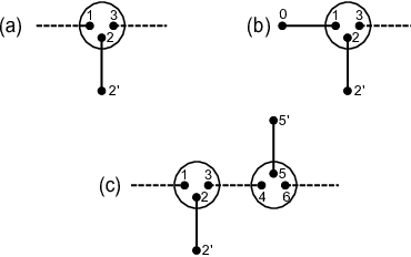
As shown in Fig. 20(a), suppose the measurement outcome on site is , then the logical basis states are and , and the logical Pauli operations could be chosen as and . Similarly, if the measurement out is , then these states and operations are , , and . The case of measurement outcome being is also similar. Note that it is possible that some spin- is connected to 2 spin-’s, as in Fig. 20(b). In this case, the encoding is the same except that the state of spin- needs to be repeated once. For instance, when the measurement outcome is , the logical becomes . The third possibility of encoding a logical qubit is that several consecutive spin- particles have the same measurement outcome, as illustrated in Fig. 20(c), where the two logical basis states could be and . Under the encoding, the ground state of every 1D AKLT quasichain can be proved to be 1D cluster state, which can be verified by the stabilizer theory as in Sec. 7.1. Furthermore, since one could simplify every logical qubit by measuring the unwanted spin-’s and spin-’s, it is reasonable to assume that every logical qubit occupies only one spin-, which has also be similarly explained in Sec. 7.1. For example, the basis state in Fig. 20(a) could be simplified from to by measuring qubit in basis .
After knowing how to obtain logical 1D cluster states, the main challenge remaining is to produce a 2D cluster state by somehow connecting them together. In order to overcome this, Cai et al. proposed the following interesting solution, as illustrated by Fig. 21.

To produce universal resource states for MBQC, for arbitrary two neighboring logical qubits and on different quasichains, one needs the capability to perform two possible operations between them: One is a logical controlled- gate defined in Eq.(8), and the other is to keep the state of every logical qubit unchanged. Cai et al. proved that both of them could be realized by operations on qubits and only, up to local operations on logical qubits and . Recall that unitary operators and measurements on qubits and are essentially corresponding operations on the spin- particle .
Without loss of generality, we assume that when producing 1D cluster states, both of the measurement outcomes on sites and are . To keep the two logical qubits unchanged, one first applies two operations on qubits and , then measures them in basis separately. If the new measurement outcomes are and , it can be checked that the effective operation is to perform and on logical qubits and respectively. Actually, this is to essentially simplify the encoding of logical qubits and by removing the unwanted spin-’s, and the resulting state might need the correction of local unitary operations.
Let us turn to the case of controlled- operation. Once more, in this case two X operations are needed on qubits and firstly, then a controlled- gate is applied on these two qubits. Up to local operations, a logical controlled- gate is implemented.
In short, we see that 1D AKLT quasichains can be connected together and then be converted to a logical 2D cluster state, which is universal for MBQC. By showing that the operations needed for related spin-’s correspond to operations on the resulting spin-’s state through the mapping in Eq.( 48), we see that that the ground state of the 2D model defined by Cai et al. can be a realistic resource state for MBQC.
8 Universal MBQC in spin- systems
In the above sections, we have seen successful examples showing the existence of spin- and spin- systems that are ideal resource states for MBQC. As the most practical quantum systems, it is natural to ask whether it is possible to find ideal resource states for MBQC from qubit systems. Unfortunately, it has been pointed out by Chen et al. that this is not the case [32].
The basic idea of Chen et al. is to show that for any two-body frustration-free qubit Hamiltonian, there always exists a ground state which is a product of single- or two-qubit states. That is to say, any entangled state cannot be the non-degenerate ground state of such a Hamiltonian, which rules out the possibility of qubit systems being ideal resource states for MBQC.
Consider an -qubit state which is genuinely entangled. That is, cannot be a product state with respect to any bipartition of these qubits. We denote the reduced density matrix of qubits and by . Consider the following Hamiltonian
| (50) |
where is the projection onto the kernel of .
It can be observed that is a two-body frustration-free qubit Hamiltonian, and is in , the ground space of . Actually, one can find that is the smallest among all the ground-state spaces of two-body frustration-free qubit Hamiltonians that contain . For a general two-body frustration-free qubit Hamiltonian , ’s might not be projections. However, we could replace them with s and the ground-state space does not change, where is the projection onto the orthogonal subspace of the ground-state space of . In this way, we only need to consider Hamiltonians composed of projections, which are of the form of Eq.(50).
Next, let us note an important point that helps with the proof. Suppose there exist nonsingular linear operators , and , where . In the language of quantum information theory, two states and can be transformed to each other via are called equivalent under stochastic local operation and classical communication (SLOCC)[58]. Note that is a ground state of if and only if is a ground state of
| (51) |
and that if one of and is product state, the other one also is. Thus, if one could show there exists a product state in the ground-state space of two-body frustration-free Hamiltonian containing , the similar situation will happen for any two-body frustration-free qubit Hamiltonian having as a ground state. Therefore, we only need to consider the SLOCC equivalent states with respect to the transformation .
We start from the simple case of three qubits. It is known that there only two different SLOCC equivalent classes for three-qubit genuinely entangled states [59], which are represented by the state
| (52) |
and the state
| (53) |
It is straightforward to check that
| (54) |
and
| (55) |
Apparently, both and contain at least one product state.
Next we proceed to the four-qubit case. Since is a genuinely entangled state, the rank of every is at most 2. We then discuss two cases: all are of rank or , or at least one is of rank .
If all are of rank or , then is actually the so-called homogenous Hamiltonian discussed in [60]. According to Lemma 2 of [60], one can always find a product of single-qubit state in the ground-state space of . We refer the readers to [60] for technical details on the discussion of homogenous Hamiltonians.
If for some pair of qubits, the rank of is . Without loss of generality, we assume to be . Now we can reduce the problem to a three-qubit case by encoding qubits and as one single qubit. Suppose is supported on two orthogonal states and . Consider the following isometry,
| (56) |
where qubits 3 and 4 are encoded by a new qubit .
Define
| (57) |
It can be seen that is also a two-body frustration-free Hamiltonian, and is still genuinely entangled. Besides, is a ground state of if and only if is a ground state of .
Since is exactly the case of three qubits we have already discussed, it follows immediately that the ground-state space of contains a product state . Let . If is product state, then is also a product state. For the case that is entangled, one can always find a product state in the range of , since this is a two-dimensional subspace of two qubits [61].
The case of qubits can just be similarly shown by induction. Thus we finally conclude that for any entangled state , there always exists a product state of single qubits which is also a ground state of . This also indicates that if we do not require that being genuinely entangled, then the ground-state space of always contains a state which is a product of single- or two-qubit states.
Therefore, we can conclude that any genuinely entangled -qubit state cannot be a unique ground state of a two-body frustration-free Hamiltonian. Because that a resource state for MBQC must be genuinely entangled, Conditions given in Sec. 4 cannot be simultaneously satisfied for any qubit system. In other words, there does not exist any idea resource state for MBQC in spin- systems.
It should be pointed out that the above discussion regarding the ground-state space properties of two-body frustration-free Hamiltonians of qubits can be strengthened further. In fact, it is shown by Ji et al. that the structure of the ground-state space of this kind of Hamiltonians can be characterized completely [33]. That is, such a ground-state space is a span of tree tensor network states of the same tree structure, which is illustrated in Fig. 22 (we refer the readers to [48] for detailed discussion tree tensor network states). Here we briefly discuss the structure given by Fig. 22 as follows. For any two-body frustration-free Hamiltonian of qubits, one can produce a corresponding special Hamiltonian , called the simplified homogenous Hamiltonian (again, we refer the readers to [60] for technical details on the discussion of simplified homogenous Hamiltonians). It can be shown that the ground-state spaces of these simplified homogenous Hamiltonians are actually spanned by (not necessarily orthogonal) product states of single qubits. In Fig. 22, every blue triangle stands for an isometry defined in Eq. 56. The very left side of the tree structure is the input, and it is the set of the product states that span the ground-state space of the corresponding simplified homogenous Hamiltonian . Then every product state solution goes through the tree structure from the left to the right, and after being operated by the meeting blue triangles, each of them becomes a solution of the original Hamiltonian . Finally, the entire ground-state space of is then spanned by these tree tensor network states.
9 Future directions
We have reviewed the recent results toward finding practical resource states for MBQC. Starting from Verstraete and Cirac’s formulation in 2004 [26] relating cluster states to VBS states, we discuss a general method for producing VBS resource states for MBQC by Gross and Eisert [20]. There has been good progress made to identify practical resource states for MBQC with VBS states. One-dimensional resource states that are useful for single-qubit MBQC are identified for spin- systems, as well as two-dimensional resource states for spin- and then later spin- systems.
Down the road there are still many interesting open threads. The no-go result by Chen et al. discussed in Sec. 8 rules out the existence of any spin- system as a practical resource state for realizing MBQC, satisfying all of Conditions given in Sec. 4. As the resource states satisfying all of Conditions are identified in Sec. 7 only for spin- systems, this naturally leaves a gap on whether a resource state satisfying all of Conditions can be identified in a spin- system. In other words, it is still unknown whether there exists a spin- state on some two-dimensional lattice which could be universal for MBQC, and at the same time is the unique ground state of some frustration-free and gapped Hamiltonian involving only two-body nearest-neighbor interactions. So far such a state has only been found for one-dimensional lattices, which does not rule out the existence of such a state on a two-dimensional lattice.
Given that the spin- systems are the most commonly found systems in nature, one would also like to seek for some relaxation of the ideal Conditions for the systems. For instance, one may try to relax the “frustration-free” condition (Condition ) or the “uniqueness” condition (Condition ) requirement by resorting to some other physical mechanisms, such as topological protection as discussed in [34, 35] or perturbation as discussed in [36, 37, 38].
In a more general theoretical framework, each one of Conditions lacks a deeper understanding. That is why the construction of each resource state discussed in this review turns out be somewhat “ad hoc”, apart from the fact that they are all VBS states.
For Condition , we would like a general understanding concerning which kinds of states could be universal for MBQC. In particular, whether the observation discussed in Sec. 4, that is, if a spin state can be reduced to a resource cluster state via adaptive local measurements at a constant cost, then is a resource state for MBQC, is in general a necessary condition for all resource states. So far, all the examples of resource states discussed in this review satisfy this condition, and indeed we use this condition to prove the universality property for MBQC for all these states. It then remains open whether a state which can be used for universal MBQC, but does not satisfy this condition, can be identified.
For Conditions and , we would like a general understanding that which kinds of quantum states can be unique ground states of two-body Hamiltonians of certain interaction patterns (for instance, two-body nearest-neighbor interactions on some kind of lattices). Recently, this problem has been linked to the certain kind of correlations of quantum states by Chen et al. in [62]. The work along the line of Chen et al. raises a general question of the so-called “from ground states to local Hamiltonians”. That is, to develop general understanding and method to find some desired local Hamiltonians to have a given quantum state as its unique ground state.
However, these local Hamiltonians constructed by Chen et al. in [62] are in general frustrated, and their discussion is restricted to finite systems (i.e., systems composed of finite particles), so whether these Hamiltonians are gapped, which is Condition , needs further discussion. It remains a general challenge to determine whether a two-body Hamiltonian is gapped, and one would like to obtain concrete examples showing whether the 2D AKLT state on the honeycomb lattice is gapped, as mentioned in Sec. 7.1.
Finally, we would like to mention that Condition , i.e., the study of ground states of frustration-free Hamiltonians, is closely related to computer science. Indeed, some of the techniques used in Sec. 8, have been used to deal with some quantum version of a computer science problem in [60]. This problem, called the quantum -satisfiability (2-SAT) problem, is of vital importance in the study of the theory of quantum computational complexity. Indeed, the characterization of the general structure of the ground-state spaces of two-body frustration-free qubit Hamiltonians shown by Fig. 22 has an immediate and interesting corollary regarding quantum computational complexity theory, i.e., the corresponding counting problem of quantum 2-SAT is equal to its classical counterpart in computational complexity, which answers an open problem raised in [63]. More details can be found in [33].
We therefore believe that these recently progresses related to MBQC with VBS states discussed in this review will not only push the effort of realizing large scale quantum computers, but also open up new directions that can further enhance the research in both quantum information science and condensed matter physics.
Acknowlegement
We thank Xie Chen and Zhengfeng Ji for helpful discussions. This work was supported in part by National Research Foundation & Ministry of Education, Singapore (L.-C. K. and Z.W.). Z.W. would also like to acknowledge the WBS grant under contract no. R-710-000-007-271. B.Z. is supported by NSERC and CIFAR.
References
- [1] R. P. Feynman. Simulating Physics with Computers. International Journal of Theoretical Physics, 21:467–488, June 1982.
- [2] D. Deutsch. Quantum theory, the Church-Turing principle and the universal quantum computer. Royal Society of London Proceedings Series A, 400:97–117, July 1985.
- [3] D. Deutsch. Quantum Computational Networks. Royal Society of London Proceedings Series A, 425:73–90, September 1989.
- [4] A. C. Yao. Quantum Circuit Complexity. Proceedings., 34th Annual Symposium on Foundations of Computer Science, pages 352 – 361, 1993.
- [5] P. W. Shor. Algorithms for Quantum Computation: Discrete Logarithms and Factoring. Proceedings., 35th Annual Symposium on Foundations of Computer Science, pages 124 – 134, 1994.
- [6] D. Cory and T. Heinrichs. Nuclear magnetic resonance approaches to quantum information processing and quantum computing. A Quantum Information Science and Technology Roadmap, v2.0, April 2004. http://quist.lanl.gov.
- [7] D. Wineland and T. Heinrichs. Ion trap approaches to quantum information processing and quantum computing. A Quantum Information Science and Technology Roadmap, v2.0, April 2004. http://quist.lanl.gov.
- [8] C. Caves and T. Heinrichs. Neutral atom approaches to quantum information processing and quantum computing. A Quantum Information Science and Technology Roadmap, v2.0, April 2004. http://quist.lanl.gov.
- [9] M. Chapman and T. Heinrichs. Cavity qed approaches to quantum information processing and quantum computing. A Quantum Information Science and Technology Roadmap, v2.0, April 2004. http://quist.lanl.gov.
- [10] P. Kwiat, G. Milburn, and T. Heinrichs. Optical approaches to quantum information processing and quantum computing. A Quantum Information Science and Technology Roadmap, v2.0, April 2004. http://quist.lanl.gov.
- [11] R. Clark D. Awschalom, D. DiVincenzo, P. C. Hammel, D. Steel, K. Birgitta Whaley, and T. Heinrichs. Solid state approaches to quantum information processing and quantum computing. A Quantum Information Science and Technology Roadmap, v2.0, April 2004. http://quist.lanl.gov.
- [12] T. Orlando and T. Heinrichs. Superconducting approaches to quantum information processing and quantum computing. A Quantum Information Science and Technology Roadmap, v2.0, April 2004. http://quist.lanl.gov.
- [13] S. Lloyd, P. C. Hammel, and T. Heinrichs. “unique” qubit approaches to quantum information processing and quantum computing. A Quantum Information Science and Technology Roadmap, v2.0, April 2004. http://quist.lanl.gov.
- [14] D. P. Divincenzo. The Physical Implementation of Quantum Computation. Fortschritte der Physik, 48:771–783, 2000.
- [15] Los Alamos National Security. A quantum information science and technology roadmap, v2.0, April 2004. http://quist.lanl.gov.
- [16] Robert Raussendorf and Hans J. Briegel. A one-way quantum computer. Phys. Rev. Lett., 86(22):5188–5191, May 2001.
- [17] A. Kitaev and C. Laumann. Topological phases and quantum computation. arXiv:0904.2771, April 2009.
- [18] E. Farhi, J. Goldstone, S. Gutmann, and M. Sipser. Quantum Computation by Adiabatic Evolution. arXiv:quant-ph/0001106, January 2000.
- [19] Michael A. Nielsen. Cluster-state quantum computation. Reports on Mathematical Physics, 57(1):147–161, 2006.
- [20] D. Gross and J. Eisert. Novel schemes for measurement-based quantum computation. Physical Review Letters, 98(22):220503, 2007.
- [21] Ian Affleck, Tom Kennedy, Elliott H. Lieb, and Hal Tasaki. Rigorous results on valence-bond ground states in antiferromagnets. Physical Review Letters, 59(7):799–802, 1987.
- [22] Gavin K. Brennen and Akimasa Miyake. Measurement-based quantum computer in the gapped ground state of a two-body hamiltonian. Physical Review Letters, 101(1):010502, 2008.
- [23] V. E. Korepin and Y. Xu. Entanglement in Valence-Bond States. International Journal of Modern Physics B, 24:1361–1440, 2010.
- [24] Xie Chen, Bei Zeng, Zheng-Cheng Gu, Beni Yoshida, and Isaac L. Chuang. Gapped two-body hamiltonian whose unique ground state is universal for one-way quantum computation. Physical Review Letters, 102(22):220501, 2009.
- [25] X. Chen, R. Duan, Z. Ji, and B. Zeng. Quantum State Reduction for Universal Measurement Based Computation. Physical Review Letters, 105(2):020502, July 2010.
- [26] F. Verstraete and J. I. Cirac. Valence-bond states for quantum computation. Physical Review A, 70(6):060302, December 2004.
- [27] T.-C. Wei, R. Raussendorf, and L. C. Kwek. Quantum computational universality of the Cai-Miyake-Dür-Briegel 2D quantum state from Affleck-Kennedy-Lieb-Tasaki quasichains. arXiv:1105.5635, May 2011.
- [28] T.-C. Wei, I. Affleck, and R. Raussendorf. Affleck-Kennedy-Lieb-Tasaki State on a Honeycomb Lattice is a Universal Quantum Computational Resource. Physical Review Letters, 106(7):070501, February 2011.
- [29] T.-C. Wei, I. Affleck, and R. Raussendorf. The 2D AKLT state is a universal quantum computational resource. arXiv:1009.2840, September 2010.
- [30] A. Miyake. Quantum computational capability of a 2D valence bond solid phase. Annals of Physics, 326:1656–1671, July 2011.
- [31] Ian Affleck, Tom Kennedy, Elliott H. Lieb, and Hal Tasaki. Valence bond ground states in isotropic quantum antiferromagnets. Communications in Mathematical Physics, 115:477–528, 1988.
- [32] J. Chen, X. Chen, R. Duan, Z. Ji, and B. Zeng. No-go theorem for one-way quantum computing on naturally occurring two-level systems. Physical Review A, 83(5):050301, May 2011.
- [33] Z. Ji, Z. Wei, and B. Zeng. Complete Characterization of the Ground Space Structure of Two-Body Frustration-Free Hamiltonians for Qubits. Physical Review A, 84(4):042338, October 2011.
- [34] A. Miyake. Quantum Computation on the Edge of a Symmetry-Protected Topological Order. Physical Review Letters, 105(4):040501, July 2010.
- [35] S. D. Bartlett, G. K. Brennen, A. Miyake, and J. M. Renes. Quantum Computational Renormalization in the Haldane Phase. Physical Review Letters, 105(11):110502, September 2010.
- [36] M. van den Nest, K. Luttmer, W. Dür, and H. J. Briegel. Graph states as ground states of many-body spin- 1/2 Hamiltonians. Physical Review A, 77(1):012301, January 2008.
- [37] S. D. Bartlett and T. Rudolph. Simple nearest-neighbor two-body Hamiltonian system for which the ground state is a universal resource for quantum computation. Physical Review A, 74(4):040302, October 2006.
- [38] S. S. Bullock and D. P. O’Leary. Bounds on Effective Hamiltonians for Stabilizer Codes. arXiv:0802.0626, February 2008.
- [39] M. Nielsen and I. Chuang. Quantum computation and quantum information. Cambridge University Press, Cambridge, England, 2000.
- [40] H. J. Briegel and R. Raussendorf. Persistent Entanglement in Arrays of Interacting Particles. Physical Review Letters, 86:910–913, January 2001.
- [41] M. A. Nielsen. Quantum computation by measurement and quantum memory. Physics Letters A, 308:96–100, February 2003.
- [42] D. W. Leung. Two-qubit Projective Measurements are Universal for Quantum Computation. arXiv:quant-ph/0111122, November 2001.
- [43] D. W. Leung. Quantum computation by measurements. arXiv:quant-ph/0310189, October 2003.
- [44] P. Aliferis and D. W. Leung. Computation by measurements: A unifying picture. Physical Review A, 70(6):062314, December 2004.
- [45] A. M. Childs, D. W. Leung, and M. A. Nielsen. Unified derivations of measurement-based schemes for quantum computation. Physical Review A, 71(3):032318, March 2005.
- [46] P. Jorrand and S. Perdrix. Unifying quantum computation with projective measurements only and one-way quantum computation. In Y. I. Ozhigov, editor, Society of Photo-Optical Instrumentation Engineers (SPIE) Conference Series, volume 5833 of Society of Photo-Optical Instrumentation Engineers (SPIE) Conference Series, pages 44–51, June 2005.
- [47] X. Zhou, D. W. Leung, and I. L. Chuang. Methodology for quantum logic gate construction. Physical Review A, 62(5):052316, November 2000.
- [48] Y.-Y. Shi, L.-M. Duan, and G. Vidal. Classical simulation of quantum many-body systems with a tree tensor network. Physical Review A, 74(2):022320, August 2006.
- [49] M. van den Nest, A. Miyake, W. D’́ur, and H. J. Briegel. Universal Resources for Measurement-Based Quantum Computation. Physical Review Letters, 97(15):150504, October 2006.
- [50] D. Perez-Garcia, F. Verstraete, M. M. Wolf, and J. I. Cirac. Matrix Product State Representations. Quantum Information Computation, 7:401, 2007.
- [51] M. Fannes, B. Nachtergaele, and R. F. Werner. Finitely correlated states on quantum spin chains. Communications in Mathematical Physics, 144:443–490, March 1992.
- [52] R. Kaltenbaek, J. Lavoie, B. Zeng, S. D. Bartlett, and K. J. Resch. Optical one-way quantum computing with a simulated valence-bond solid. Nature Physics, 6:850–854, November 2010.
- [53] F. Verstraete, M. M. Wolf, D. Perez-Garcia, and J. I. Cirac. Criticality, the Area Law, and the Computational Power of Projected Entangled Pair States. Physical Review Letters, 96(22):220601, June 2006.
- [54] D. Perez-Garcia, F. Verstraete, J. I. Cirac, and M. M. Wolf. PEPS as unique ground states of local Hamiltonians. Quantum Information Computation, 8:0650, 2008.
- [55] D. Gottesman. Stabilizer codes and quantum error correction. Ph.D. thesis, Caltech, 2004.
- [56] A. S. Darmawan, G. K. Brennen, and S. D. Bartlett. Measurement-based quantum computation in a 2D phase of matter. arXiv:1108.4741, August 2011.
- [57] J. Cai, A. Miyake, W. Dür, and H. J. Briegel. Universal quantum computer from a quantum magnet. Physical Review A, 82(5):052309, November 2010.
- [58] Charles H. Bennett, Sandu Popescu, Daniel Rohrlich, John A. Smolin, and Ashish V. Thapliyal. Exact and asymptotic measures of multipartite pure-state entanglement. Phys. Rev. A, 63(1):012307, Dec 2000.
- [59] W. Dür, G. Vidal, and J. I. Cirac. Three qubits can be entangled in two inequivalent ways. Phys. Rev. A, 62(6):062314, Nov 2000.
- [60] S. Bravyi. Efficient algorithm for a quantum analogue of 2-SAT. arXiv:quant-ph/0602108, February 2006.
- [61] K. R. Parthasarathy. On the maximal dimension of a completely entangled subspace for finite level quantum systems. arXiv:quant-ph/0405077, May 2004.
- [62] J. Chen, Z. Ji, B. Zeng, and D. Zhou. From ground states to local Hamiltonians. arXiv:1110.6583, November 2011.
- [63] S. Bravyi, C. Moore, and A. Russell. Bounds on the quantum satisfibility threshold. arXiv:0907.1297, July 2009.