An Investigation of Sloan Digital Sky Survey Imaging Data and Multi-Band Scaling Relations of Spiral Galaxies (with Dynamical Information)Note: Submitted to MNRAS 2011, not for distribution
Abstract
We have compiled a sample of 3041 spiral galaxies with multi-band imaging from the Sloan Digital Sky Survey (SDSS) Data Release 7 and available galaxy rotational velocities, , derived from HI line widths. We compare the data products provided through the SDSS imaging pipeline with our own photometry of the SDSS images, and use the velocities, , as an independent metric to determine ideal galaxy sizes () and luminosities (). Our radial and luminosity parameters improve upon the SDSS DR7 Petrosian radii and luminosities through the use of isophotal fits to the galaxy images. This improvement is gauged via and relations whose respective scatters are reduced by 8% and 30% compared to similar relations built with SDSS parameters. The tightest relations are obtained with the -band radius, , measured at 23.5 mag arcsec-2, and the luminosity , measured within . Our scaling relations compare well, both in scatter and slope, with similar studies (such comparisons however depend sensitively on the nature and size of the compared samples). The typical slopes, , and observed scatters, , of the -band , and relations are , , , and , , . Similar results for the SDSS and bands are also provided. Smaller scatters may be achieved for more pruned samples. We also compute scaling relations in terms of the baryonic mass (stars + gas), , ranging from to . Our baryonic velocity-mass () relation has slope and a measured scatter dex. While the observed and relations have comparable scatter, the stellar and baryonic relations may be intrinsically tighter, and thus potentially more fundamental, than other relations of spiral galaxies.
Keywords:
galaxies: dynamics —galaxies: formation —galaxies: kinematics —galaxies: spirals —galaxies: structure —dark matterI Introduction
Fundamental scaling relations for spiral galaxies are known to emerge from the combination of observed galaxy rotation velocity, , total luminosity , and size, . For instance, the relation, also known as the Tully-Fisher relation (Tully & Fisher 1997), probably defines the fundamental plane of spiral galaxies. That is, the scatter of the relation cannot be reduced by considering any other third parameter (e.g., Courteau & Rix 1999, hereafter CR99; Courteau et al. 2007, hereafter C07; Dutton et al. 2007, hereafter D07; Pizagno et al. 2007). The study of galaxy scaling relations also enables a direct comparison with theoretical models of galaxy formation (e.g., Pizagno et al. 2005; D07; Avila-Reese et al. 2008, hereafter AR08; Dutton & van den Bosch 2009; Dutton et al. 2011, hereafter D11). These and other studies suggest that the simultaneous matching of the and relations, whilst matching the observed galaxy luminosity function and reproducing the shape of galaxy surface brightness profiles is a challenging task. For example, for standard disk galaxy models (e.g., Mo, Mao & White 1998; D07) with standard stellar initial mass functions (i.e., Kroupa 2001/Chabrier 2003) to match basic galaxy scaling relations, D07 and D11 showed that halo expansion is required. This may be realized through dynamical friction on baryonic clumps and/or supernova driven mass outflows (e.g., Navarro, Eke, & Frenk 1996; El-Zant, Shlosman, & Hoffman 2001; Mo & Mao 2004; Governato et al. 2010; Cole, Dehnen & Wilkinson 2011).
It has also been stated that the luminosity of a spiral galaxy is a poorer tracer of its circular velocity than baryonic mass, (McGaugh et al. 2000; McGaugh 2005). The latter is defined as the sum of the luminous mass, , and the gas mass, . is usually obtained by multiplying the total extrapolated luminosity, measured in a specific wave band, by a suitable stellar mass-to-light () ratio. is measured directly from the HI flux, using a correction factor of 1.4 to account for the mass fraction of helium. At low total galaxy mass, can be a significant fraction of , thus raising the question whether , or is a better match to . The latter, which is also known as the “baryonic Tully-Fisher” or “BTF”, may also have a different slope than the standard relation (Bell & de Jong 2001; Verheijen 2001; McGaugh 2005; Gurovich et al. 2010). The samples that have been used for BTF studies have typically included fewer than galaxies based largely on multiple, heterogeneous samples. For their sample of 243 galaxies, McGaugh et al. (2000) found that the BTF relation is more “fundamental” than the relation; deviations from the BTF relation may however exist (McGaugh & Wolf 2010). However, a BTF relation based on a large, statistical sample of galaxies is still lacking. The discrepancies between published BTF slopes and scatters also motivate a new study with as large a galaxy sample with accurate rotation velocities and HI fluxes as possible.
Interest in galaxy scaling relations also stems from wanting accurate distance estimators, which in turn is obtained via the suitable pairing of a distance-dependent and distance-independent galaxy parameters such as size, luminosity or colour with circular velocity. The infrared relation has typical distance errors of (e.g., Aaronson et al. 1979; Pierce & Tully 1988; Gavazzi et al. 1999; Masters et al. 2006; hereafter M06; Saintonge & Spekkens 2011; hereafter SS11). Very large data samples and carefully measured galaxy parameters can reduce sampling error in these studies. The Sloan Digital Sky Survey (Abazajian et al. 2009; hereafter SDSS) is currently the largest data base of galaxy structural parameters11 1 The NYU Value-Added Galaxy Catalogue by Blanton et al. (2005) also offers a cross-matched collection of galaxy catalogs, using the SDSS library as a core.. It is thus relevant to ask if the SDSS library of galaxy scaling parameters yields the tightest possible scaling relations.
A main goal of this paper is indeed to investigate the quality of galaxy scaling relations based on size, luminosity, and colour derived from SDSS data products. The intent is to compare SDSS pipeline data products with similar measurements extracted from SDSS images but using independent data reduction methods.
We develop our analysis of relations through two specific channels: i) we first compare the multi-band data products from the SDSS DR7 with our own galaxy structural parameters extracted from SDSS FITS galaxy images, and ii) we determine which of the parameters yield the tightest luminous and baryonic scaling relations. Limitations of the SDSS data products will be addressed along the way (see also Masjedi et al. 2006; Lauer et al. 2007; Fathi et al. 2010).
To set the foundations of the relation, we follow Courteau et al. (2007, hereafter C07) whose sample comprised 1300 late-type galaxies. The sample that we present here, having more than galaxies, is a two-fold increase over C07. We follow most, though not all, of the reduction methods and parameter corrections from C07. For instance, C07 used photometry and rotational velocities from four separate sources (Mathewson et al. 1992; Tully et al. 1996; Dale et al. 1999; Courteau et al. 2000). A significant improvement of this study over C07 is our use of strictly homogeneous data for both the multi-band photometry (SDSS) and line widths (S05/S07). C07 also used disk scale lengths as a measure of galaxy size in order to facilitate comparisons with galaxy formation models (D07). We consider disk scale lengths here as well, but will also extract other radial metrics that yield tighter relations (see also SS11).
The available SDSS parameters that are of interest to us, namely the galaxy size, , and luminosity, , are both distance-dependent. Thus, in order to test which of our measurements or the SDSS parameters yield the tightest scaling relations, we must compare each value against an independent metric which we take here as the distance-independent galaxy velocity.
Our study benefits from the availability of rotational velocities, , from spatially-unresolved neutral hydrogen (HI) 21 cm spectral line widths, for nearly 9000 spiral galaxies (Springob et al. 2005; hereafter S05; Springob et al. 2007, hereafter S07). Cross-correlation of the S05 and S07 line width catalogs with the SDSS will define our target sample.
Our paper is organised as follows: In Section II, we cross-correlate the S05 and S07 HI line width catalogs with the SDSS DR7; this yields a sample of 3041 disk galaxies with accurate photometry and line widths. We discuss the extraction of radial and luminous parameters from SDSS images in Section III. Final galaxy parameter corrections are applied in Section IV and the data table of galaxy structural parameters is presented in Section V. In Section VI, we compare the SDSS and our galaxy parameters against an independent foil, here chosen to be the (distance-independent) rotational velocity, , from S05/S07. We determine the “best” scaling parameters with which to build the tightest relation in Section VII and present, in Section VIII, the largest baryonic Tully-Fisher sample to date. A summary of our results is presented in Section IX.
II Data Sample
In order to simultaneously test the reliability of SDSS data products and establish the most comprehensive scaling relations to date, we seek not only the largest but the most homogeneous compilation of galaxy structural parameters to date. This can be done through the cross-correlation of the large compilation of 9000 galaxies within km s-1with HI line widths by S05 and S07 with the multi-band photometry provided by the SDSS.
The SDSS archive query with S05/S07 targets yielded FITS images for 4260 galaxies. That sample was examined visually to eliminate galaxy pairs, interacting galaxies and images with bright foreground stars, and any galaxy whose light profile could not be extracted (e.g., very faint targets). Due to the survey nature of the SDSS, target galaxies may often appear close to the edge of the CCD image frame and subsequently compromise the photometric analysis. A large fraction ( 40%) of the more luminous galaxies in our sample which suffer from these “edge effects” had to be discarded.
We were left with a final sample of 3041 galaxies for which both S05/S07 rotational velocities and acceptable SDSS FITS images are available. We have subdivided this large sample, dubbed “Sample A”, into three subsets (Samples B, C, D) to investigate the effects of distance uncertainties and inclination on galaxy scaling parameters.
The main sample and subsets include the following systems:
- (A)
Full Sample - 3041 galaxies from S05/S07 found in SDSS DR7 with imaging suitable for surface photometry;
- (B)
Best Inclinations - 1725 galaxies from Sample A with moderate inclinations . This removes the nearly face-on galaxies that would suffer from large uncertainties in their deprojected rotational velocity, as well as the more inclined galaxies () whose disk may be significantly obscured by line-of-sight dust and whose surface area for isophotal photometry is barely visible;
- (C)
Best Distances - 1076 galaxies in Sample A with the best distance determinations from high quality spectroscopic data of S07 (referred to as “SFI++” by S07);
- (D)
Best Inclinations and Distances - 652 galaxies from the intersection of Samples B and C. Sample D is thus our “Best Sample”.
III Light Profile Extraction
III.1 SDSS FITS Image Photometry
We extract light profiles from the SDSS images of all the Sample A galaxies using the surface brightness profile extraction methods presented in Courteau (1996) and adapted to SDSS images by McDonald et al. (2009; 2011). Given the lower signal-to-noise of the SDSS and bands (Blanton et al. 2001), our analysis will rely strictly on the bands.
The image processing software XVISTA22 2 see http://ganymede.nmsu.edu/holtz/xvista/ is the backbone of our surface brightness profile calculations. The XVISTA command PROFILE was used to fit azimuthally-medianed elliptical isophotes through the galaxy 2D light distribution. The position angle and ellipticity of each isophote could vary while the centre was kept fixed. The ellipticity which best defines the stable outer disk was visually determined and the isophotal solution was extended to faint light levels using that ellipticity to extract the deepest profile possible. The surface brightness was calculated from the median sky-subtracted flux level over an elliptical contour. Intervening stars were masked and isophotal twists due to bright spiral arms were also smoothed out by hand.
The higher signal-to-noise of the -band SDSS images, and the lesser sensitivity of galactic dust at redder wavelengths, make the -band the filter of choice for galaxian surface photometry. The profile templates (position angle and ellipticity) for each galaxy is based on the -band image and then applied to both and images. This ensures that galaxy colour profiles are extracted over the same physical regions of a galaxy. The surface brightness levels at each pixel were computed in each band and scaled using the photometric zero-point, airmass and extinction coefficients supplied in the SDSS-drObj photometric calibration files. The surface brightness profiles for the 3041 galaxies in Sample A were all inspected individually for quality control.
III.2 SDSS Sky Measurements
The galaxy light profiles were all sky-subtracted; this operation being clearly the largest source of error in surface brightness extraction. The SDSS image headers already include an estimate of the sky background level. However, the sky backgrounds for bright extended galaxies in the SDSS DR1 - DR7 are known to be systematically over-estimated resulting in the under-estimation of galaxy fluxes and sizes by as much as 20-30% (Masjedi et al. 2006; Lauer et al. 2007; Abazajian et al. 2009; McDonald et al. 2011). Conversely, for fainter systems such as LSB galaxies, West et al. (2010) report an over-subtraction of the sky level in the SDSS photometric pipeline. We now present our investigation of sky subtraction uncertainties based on DR7 SDSS -band galaxy images33 3 Note that background subtraction improvements in DR8 have resulted in more reliable photometry of large galaxies (Blanton et al. 2011). The treatment about sky uncertainties presented in our paper is still relevant for smaller galaxies, whether in DR7 or DR8..
The SDSS sky background level, , is measured from an initial estimate of the median pixel value of every fourth pixel in the image clipped at 2.3 , where is the rms noise of the image. The brightest stars, but not necessarily their wings, are thus removed from the image and the sky level is recomputed to provide a final background estimate. The different sky levels as provided by SDSS for Sample A galaxies are shown in Figure 1 for the three SDSS bands.
To investigate the deviations in sky measurements, we compute two other sky measurements from the SDSS -band FITS images: i) , is the median pixel value over the full image frame and, ii) is the median sky background level from five boxes placed interactively away from the galaxy image. The latter was computed for a sample of 30 galaxies with the largest and smallest angular sizes. In principle, provides the most realistic estimate of the sky background.
We measure the difference sky in -band sky levels with respect to as,
| (1) |
Figure 2 shows the results for and for our subsample of 30 selected galaxies. First, we note that the largest deviations in both panels are for galaxies whose angular diameter exceeds 75. Fortunately, most of our galaxies have much smaller sizes.
The top panel of Figure 2 confirms that the SDSS sky levels are overestimated with respect to our “best” estimates, . The percent difference for most small galaxies is however less than 0.2%. The offset between the “Full Sky” estimate and our best sky measurement (bottom panel) is surprisingly comparable to that with the SDSS sky level (top panel). In most cases, the deviations are less than %.
The effect of over- and under-subtracted skies on a typical light profile is shown in Figure 3 for sky background errors at the 0.2% (light blue points), 0.5% (dashed line) and 1.0% (dark solid line) levels on the -band surface brightness profile of UGC 5651 (an intermediate-size Sc galaxy centered on the image frame). The dashed black line marks the mag arcsec-2 level and it can be seen that most isophotal measurements above the mag arcsec-2 level are largely free of normal sky subtraction errors. We will compute in Section VI.2 the effect of sky subtraction errors on measured sizes and fluxes.
Based on these tests, we have adopted the SDSS sky levels, , for the sky background subtraction of our surface brightness profiles. Caution must still be taken when utilizing SDSS sky background estimates, especially for large galaxies.
Figure 4 shows the median surface brightness errors versus median surface brightness in the bands for all the galaxies in Sample A. Our sky-subtracted galaxy light profiles are quite stable and reliable down to surface brightnesses of mag arcsec-2, where surface brightness errors typically do not exceed 0.4 mag arcsec-2.
III.3 Structural Parameter Extraction
We now present the measurements of structural parameters in the bands for the 3041 galaxies in Sample A. We seek isophotal, effective and physical size and luminosity parameters for the construction of relations.
Isophotal parameters are measured at a specific surface brightness level, effective parameters are measured at a radius which encloses half of the total light, and physical sizes can refer to a disk scale length or an exact radius in kpc.
The total luminosity of a galaxy can be estimated by extrapolating its light profile to infinity assuming an extended exponential disk. Given that the SDSS photometry is already fairly deep (Figure 4), the profile extrapolation adds only a few percent of the light to the total. The exponential disk model is given by
| (2) |
where is the extrapolated central surface brightness in counts and is the scale length of the exponential disk. In magnitude units, Equation (2) becomes
| (3) |
where the units of are mag arcsec-2. The disk light, , in counts, is the cumulative surface brightness under the exponential fit from to infinity,
| (4) |
Disk extrapolation fits are highly susceptible to the fit baseline and the presence of spiral arms. Indeed, disk scale lengths () and central surface brightnesses () may vary by as much as 20% from author to author (Knapen & van der Kruit 1991; Courteau 1996; Courteau et al. 2011). Here we adopt the interactive “marking the disk” technique to fit an exponential function to the disk surface brightness profile (Giovanelli et al. 1999; C07). The inner and outer radii for the fit baseline encompass the region of the SB profile that is dominated by the disk. Full 2D bulge-disk model decompositions of the SDSS images will be reported elsewhere; for our current purposes, the “marking the disk” technique is fully adequate.
Besides the measurement of a disk scale length and disk central surface brightness, we can also compute from these fits the isophotal radius, , and apparent magnitude, m23.5, within the 23.5 mag arcsec-2 isophote. This straightforward measurement does not depend on any disk fitting or parameterisation. Other isophotal radii can be measured but can be shown to yield smallest scatter of the RL relation (e.g., Courteau 1996; Section VI.2).
We also compute the half-light (or effective) radius containing 50% of the total extrapolated light. The effective surface brightness is defined as . We also define other parameters: mext is the total magnitude of the extrapolated light profile and m2.2 the magnitude integrated within the radius . The latter corresponds to the peak of the rotation curve of an idealized pure exponential disk (e.g., Freeman 1970; Binney & Tremaine 1987).
We now have various sets of radii and apparent magnitudes based upon our extrapolated light profiles for 3041 galaxies in , and -bands. Colours can also be computed from various magnitude combinations. In Section VI we quantify the robustness of these structural parameters in the context of the scaling relations.
Our analysis benefits from the independent reduction of 211 galaxy light profiles by two of us (MH and YZ). The light profiles for nine of these galaxies are presented in Figure 5 as blue (reduced by MH) and red (reduced by YZ) profiles. Comparing these profiles shows that differences between MH and YZ, if any, are small and purely random, despite slightly different treatments in the few interactive aspects of the SB profile extraction. These two treatments differ only in the smoothing of isophotal twists and luminosity extrapolation of the outer disk (see Section III.2). MH extracted the light profiles for all 3041 galaxies in Sample A and we adopt her final catalog. The extensive comparisons with YZ reinforce the reliability of our sample.
IV Final Data Corrections
We now correct the extracted structural parameters (e.g., sizes, luminosities, surface brightnesses) following the prescription of C07 but now accounting for the SDSS filter system. The velocities derived from the HI line profiles are corrected according to the prescriptions of S05 and S07. The inclination of each galaxy is measured from the ellipticity of the outer disk isophotes of the SDSS -band image and corrected for projection effects using Holmberg’s oblate spheroid description,
| (5) |
where the ellipticity, , is the axial ratio of a galaxy viewed edge-on, and are the disk major and minor axes, and is the polar axis.
In order to determine the variation of projected ellipticity with colour or morphological type, we have used the Galaxy Zoo classification (Lintott et al. 2008). We selected all of our galaxies classified as edge-on by % of all the Galaxy Zoo survey participants (and eliminated all those classified as ellipticals or merger by % of them) yielding a sample of 1377 candidate edge-on galaxies. We then visually inspected the SDSS images for all these galaxies and eliminated a further 506 systems deemed not perfectly edge-on. For each of the remaining 871 edge-on galaxies, an ellipticity was computed using the adaptive second moments, and , provided by the SDSS pipeline. From these moments, the adaptive ellipticity was computed following Kautsch (2009). Finally, this ellipticity was converted to an axial ratio ().
Figure 6 shows the variation of SDSS-derived axial ratios in the -band versus mean galaxy colour, computed at the effective radius, for 871 edge-on galaxies each depicted as a black dot. The morphological correspondance (top axis) was derived from SDSS colours tabulated in McDonald et al. (2011). The red dots are median averages per given morphological bin. The trend of naturally increases with redder, progressively bulge-dominated galaxies. The distribution is relatively flat for blue (late-type) galaxies, with an upturn at , corresponding to Sa/S0a galaxies. Several S0 galaxies have , reminiscent of the Sombrero galaxy. The few late-type systems with are likely a failure in the adaptive moment pipeline. Note that similar distributions are obtained for the and bands.
Based on Figure 6, we adopt as the minimum axial ratio, and thus intrinsic thickness, of spiral galaxies. This value agrees with a similar study by Giovanelli et al. (1994), though a value as high as 0.2, as reported by Lambas et al. (1992), is also realistic considering the intrinsic errors on galaxy radii. For their study of the baryonic Tully-Fisher relation (see Section VIII), Stark et al. (2009) adopted . The effect of using or 0.2 is inconsequential for our study.
The apparent (-band) magnitudes have been homogeneously corrected for internal extinction , external galactic extinction and -correction according to
| (6) |
The inclination-dependent internal extinction correction in magnitudes is given by
| (7) |
where is interpolated in the , and bands from the corrections of Tully et al. (1998) given the corrected line widths from S05,
| (8) | |||
| (9) | |||
| (10) |
The Galactic extinction, , from Schlegel et al. (1998) is provided by the SDSS. The cosmological -correction, , is calculated from the template of Blanton & Roweis (2007) for each SDSS filter.
The absolute magnitudes, , are calculated in their respective band as
| (11) |
where the Hubble constant km sec Mpc (Komatsu et al. 2011) and is the distance in kpc derived from the velocities in the rest frame of the cosmic microwave background, , as compiled by S05 and S07. For calibration to solar units, we use =5.12, =4.68 and =4.57 (York et al. 2000); we use in the conversion from apparent to absolute quantities.
We correct both effective () and central () surface brightnesses for internal and external extinction following C07:
| (12) | |||
| (13) |
These are reported in a data table (Table 1 as presented Section V) but not used for further analysis in this paper, except in Figure 22. Radii measurements may be corrected following Giovanelli et al. (1995), as also reported in C07. However, we shall find in Section VII.2 that such corrections do not yield a reduction of the and relations scatter. In view of the uncertain nature of most radial scale corrections, our analysis relies on uncorrected radii.
IV.1 Parameter Uncertainties
We follow M06, C07, AR08, SS11 and many other studies of galaxy scaling relations in estimating the uncertainties for each scaling relation parameters , and . Uncertainties in assume 10-15% errors for each of the parameters , , , and in Equation (6). That is,
| (14) |
where is the statistical error in the raw magnitude measurement. A more complete assessment of parameter errors is found in SS11. Our results are however practically the same.
Typical measurement errors on amount to 20%, or dlog. This value is also obtained by M06 and SS11 for their measurements of the absolute luminosity, , in the -band. The uncertainties on the rotational velocities as compiled by S05/S07 amount to 5%, or dlog (SS11 use dlog). We also assume a 15% uncertainty, or dlog on disk scale lengths (e.g., MacArthur et al. 2003; Courteau et al. 2011) and a 7% error, or dlog=0.03, on isophotal radii (same as SS11).
In the fits that follow (Section VII), the quantities dlog and dlog are computed independently for each galaxy while dlog for various radii measurements (, , ) is set to the mean values above for each galaxy. Using this method or assigning a constant error to each parameter plays no role in the final scaling relations.
V Data Table
We now present our extensive compilation of galaxy structural parameters. The recessional and rotational velocities, HI flux, and morphological classification are from S05/S07. All other structural parameters have been derived by us from SDSS images as described in Section III.3. The distribution of several of these parameters is shown in Figure 7 for the full Sample A in red and for our Sample D with best constrained distances and inclinations in blue. Figure 7 shows a broad parameter coverage, though none of which can be deemed complete. The parameter distributions are roughly (log-)normal with an emphasis on Sb/Sc morphological types.
Table 1 gives a list of structural parameters for all the Sample A galaxies. The first few entries of the catalog are shown here; please see the electronic version for the full list. The entries are arranged as follows:
- Col. (1):
-
UGC or AGC galaxy name;
- Col. (2):
-
, the corrected galaxy inclination in degrees using in Equation (5);
- Col. (3):
-
, the recession velocity of the galaxy relative to the cosmic microwave background frame in km s-1 as calculated by S05 and S07. The S07 estimates of supersede S05 in the case of multiple measurements;
- Col. (4):
-
, the corrected rotational velocity in km s-1 from the HI line width profiles measured at 50% of total flux by S05 & S07 (). S05/S07 line widths are corrected for instrumental effects and redshift broadening. is corrected for the inclination of the disk and distance but not for turbulent motion in the HI gas. Sample D uses only rotational velocities from S07;
- Col. (5):
-
T, the RC3 morphological type as listed by S05 & S07;
- Col. (6):
-
, the half-light radius based on the total extrapolated -band luminosity of the galaxy in arc seconds;
- Col. (7):
-
, the radius at the -band 23.5 mag arcsec-2 isophote in arc seconds;
- Col. (8):
-
, the disk scale length of the galaxy in arc seconds;
- Col. (9):
-
m, the total apparent magnitude of the galaxy including the extra light from the disk extrapolation to infinity;
- Col. (10):
-
m, the apparent magnitude within the -band 23.5 mag arcsec-2 isophote;
- Col. (11):
-
m, the apparent magnitude within 2.2 of the surface brightness profile. Non-entries in this column are due to a failed disk extrapolation, described in Section VI.3;
- Col. (12):
-
, the corrected central surface brightness in mag arcsec-2;
- Col. (13):
-
, the corrected effective surface brightness measured in mag arcsec-2;
- Col. (14):
-
, the colour of the galaxy calculated from the difference in and extrapolated magnitudes ;
- Col. (15):
-
, the colour of the galaxy from the and bands as above;
- Col. (16):
-
, the galaxy light concentration, , where and enclose 20% and 80% of the extrapolated -band light, respectively;
- Col. (17):
-
, the neutral hydrogen gas mass in derived by S05 from the corrected HI line flux measurements;
- Col. (18):
-
, the stellar mass of the galaxy in units of from the extrapolated -band luminosity times the stellar mass-to-light ratio prescription of Bell et al. (2003) with a Chabrier (2003) IMF;
- Col. (19):
-
, the baryonic mass of the galaxy in units of . Section VIII discusses the sum of the stellar, HI and gas masses to make up the total baryonic mass, ;
- Col. (20):
-
, the total mass of the galaxy computed at according to where is the radius in kpc and is the observed rotation velocity in km s-1.
VI SDSS Comparisons
Below, we compare our detailed structural parameters extracted from SDSS galaxy images with SDSS pipeline data products for the same galaxies.
VI.1 The SDSS Data Products
The SDSS measurements of interest to us are the , , and band Petrosian parameters. The Petrosian radius, , is the radius at which ratio of the local surface brightness averaged over the annulus is equal to 0.2 times the mean surface brightness within as measured by the automated SDSS pipeline (Blanton et al. 2001; Strauss et al. 2002; Yasuda et al. 2001). The Petrosian magnitude, mp, is measured within the aperture of radius 2. The Petrosian radii and encompass 50% and 90% of the total light measured within 44 4 The online SDSS archive tags are petroRad, petroR50, petroRpn and petroMag..
We first find that the SDSS data products are burdened by the mis-identification of galaxy objects in the SDSS SQL query method, leading to erroneous measurements of radius and light for numerous objects. Some of the faulty measurements are due to the “shredding” caused by the deblending algorithm in the SDSS reduction pipeline. Overlapping objects are deblended to separate underlying components and extract proper measurements. Occasionally large galaxies may be interpreted as multiple systems and are thus “shredded” by the algorithm. The 1% “shredding” occurrence in the SDSS DR1 reported by Blanton et al. (2001) is also found in DR7. We confirmed this “shredding” effect in the SDSS DR7; we found object-type mis-identifications for objects classified as galaxies that are either star-forming regions or foreground stars, both of which are more concentrated than a typical galaxy.
To identify the deviant SDSS pipeline data, we plot in Figure 8 the logarithmic difference between the 90% and 50% light radii, , in the -band against both the magnitude mp in the upper panel (a) and the logarithmic Petrosian radius, , in the lower panel (b). The clear separation at , shown as a dashed vertical line, is the clear distinction between correctly identified galaxies and the mis-identified compact objects. Objects located left of this line were discarded.
We also examined the -band Petrosian radii and their associated errors. Faulty computations of the Petrosian radius or magnitude are given a default -1000 error; those are shown as red crosses in Figure 8. Many failed calculation of Petrosian radius are given a SDSS default value of 3 arc seconds; hence the horizontal array of crosses near in panel (b). These faulty measurements apply mostly to faint galaxies whose flux is below a nominal threshold within the Petrosian aperture.
Thus, we weed out SDSS data based on the following criteria: i) mis-identified non-galaxian objects with , and ii) failed computation of the Petrosian radius with errors of arc seconds in the -band. This eliminates 14% of the SDSS pipeline data products; we are left with a “clean” SDSS sample of 2605 galaxies.
The computation of SDSS data products within a circular aperture compared to our structural parameters extracted from isophotal ellipse fitting is an additional source of confusion in the comparison of our data. Circular and isophotal apertures clearly measure different portions of the galaxy. Projection effects for a galaxy bulge and disk within a circular or elliptical aperture yield very different luminosity profiles (e.g., Bailin & Harris 2009).
Such inclination effects between the SDSS Petrosian half-light radius, , and the half-light radius, , measured from isophotal fitting are explored in Figure 9. The Petrosian radius is systematically smaller than . More importantly, this offset increases with inclination, from red crosses ( to blue circles () in Figure 9, as the Petrosian aperture progressively samples less light (compared to the isophotal aperture) at higher tilt. Slight curvature may also be detected in each inclination distribution but overall, there exists a direct mapping between and as a function of inclination. The scatter between a Petrosian radius and an isophotal radius is entirely dominated by inclination.
VI.2 Comparison of Radial Measurements
We now compare the “clean” -band SDSS Petrosian radii for 2605 galaxies with our suite of radial parameters, namely , and computed for Sample A (Section III). Figure 10 shows the raw Petrosian radial measures , and from the SDSS pipeline against two of our own radial measurements and , extracted from our -band light profiles. The red dashed lines have slope unity.
We first observe that inclination drives the scatter in all the correlations between Petrosian (i.e. circular) and isophotal (i.e. elliptical) radii although that effect is strongest for . Of course, no such dependence is seen for versus as both measures are derived from isophotal fits. There is also no one-to-one correlation between our radial measures and the SDSS Petrosian radii. Therefore, any scaling relation based on SDSS or isophotal sizes ought to yield different parameters (slope, zero-point, scatter).
The Petrosian radius correlates well with the two other Petrosian radii and , as one might expect since the latter two derive from . The bright end of the diagrams involving Petrosian radii could be slightly skewed to smaller values due to the reported over-sky subtraction errors for large objects (see Section III.2). The effect of an over-subtracted sky on the measured isophotal radii, and fluxes, was demonstrated in Figure 3 for the sample galaxy UGC 5651.
Table 2 presents the propagated error in radius and as well as the magnitude differences m23.5 and mext due to sky uncertainty. A 0.2% sky error typically yields 1-2% radial scale variations or magnitude differences less than 0.03 mag. These small values are representative of our data; 1% sky errors would be dramatic but they are, fortunately, unrealistic. As observed earlier (Section III.2), the isophotal parameters, and m23.5 are least affected by typical sky background errors.
Figure 10 highlights the comparison and differences between radii derived from circular and isophotal apertures. However, to decide which of these measurements yields the tightest galaxy relations requires an objective comparison against an uncorrelated variable, here chosen to be the deprojected rotational velocity, . Figure 11 shows the distribution of data for each -band radial parameter; Sample A (all the available data) is shown with gray points overplotted whereas Sample D (best inclination and distance data) is in black. The top panels show scaling relations with isophotal radii and the disk scale length; similarly for the bottom panels with Petrosian radii for the clean SDSS sample. The red dashed line in each panel is an orthogonal linear fit, with bootstrap re-sampling (see C07), of the relations for Sample D.
We evaluate the tightness of each fit with both the one- standard deviation about the best orthogonal fit and the Pearson coefficient. The listed values of and are those for Sample D.
The tightest relation is clearly that which involves , in agreement with Saintonge et al. (2008) and SS11. We discuss their results in Section VII. Of the Petrosian radii, , yields the tightest relations.
Figure 12 shows the variation of for the three radii shown in green, yellow and red colours respectively. The four sub-samples are plotted as A (circles), B (triangles), C (squares) and D (stars). The vertical dashed line separates our radial measurements from the SDSS Petrosian radii.
Overall, Sample C and D yield comparably tight relations indicating that the inclination cuts in Sample D do not improve the trends for the relation significantly. Other relations with , and the Petrosian radii are however improved when high and low inclinations are weeded out. Still, the biggest effect in obtaining a tighter relation results from eliminating galaxies with uncertain distances.
Parameters derived from the extrapolated light profiles, such as and , are especially sensitive to the vagaries of the “disk-like” exponential region in such profiles. Indeed both and show a poorer scatter in Figure 12. is also affected by projection effects, internal extinction by dust and stellar populations. For instance, there is a real dust extinction gradient from center (opaque) to edge (transparent) in galaxy disks. The measured scale lengths are larger, and central surface brightnesses are smaller than their intrinsic dust-free values. Empirical corrections (Giovanelli et al. 1995; Masters et al. 2003; Graham & Worley 2008) or corrections based on radiative transfer models (Popescu et al. 2005; Driver et al. 2007; Gadotti et al. 2010) for extinction effects on as a function of inclination have been proposed, but these remain grossly uncertain.
The isophotal radius is the clear winner with this test, for all bands and all samples. The SDSS Petrosian radius, , also fares well though the unreliable object identification and deprojection effects for tilted galaxies (Section VI.1) make the interpretation of this parameter less simple than .
In seeking a direct match with galaxy formation models (e.g., Mo, Mao, & White 1998; D07; D11), numerous scaling relation studies have relied on as the fiducial galaxy size (e.g., C07 and references therein). This is because the scale length indicates the change of surface density with radius for any galaxy; as a global tracer of galaxy structure, is a straightforward prediction of galaxy formation models. Different stellar populations however have different scale lengths. The space density of a given stellar population in a disk is mostly controlled by the angular momentum evolution of that disk (Foyle et al. 2008; Rov skar et al. 2008; Dutton 2009). , which measures the local surface density of a disk, is also sensitive to the local stellar populations (see Figure 13). The local space density is more sensitive to local star formation conditions than those averaged at .
Whether or is preferred for either the tightest relation that it yields or for a more direct connection with theory, the interpretation of the relation relies on a full understanding of the biases that each method entails.
VI.3 Comparison of Luminosity Measurements
In order to determine the best luminosity measure from circular (Petrosian) or elliptical apertures, we compare the clean SDSS Petrosian apparent magnitudes, mp, against our suite of derived apparent magnitudes m23.5, mext, md and m2.2. Figure 14 shows these five -band measurements against each other; the red dashed line has slope unity.
The top row in Figure 14 shows that the best match with the Petrosian magnitude, mp, is obtained with . The top panels all show a departure from the one-to-one line at the bright end. This is still due to the “shredding” effect (see Section VI.1) for large galaxies. For non-shredded systems, the Petrosian flux accounts for 98% of the total flux of a galaxy (see Shen et al. 2003).
The disk magnitude md shows the largest scatter with other luminosity measurements, as it is tied to the uncertain disk scale length via Equation (2) and does not account for the bulge luminosity. A superb correlation between and exists; however yields noisier correlations.
In Figure 15 we examine which -band luminosity parameter yields the tightest scaling relation. The dashed red line is the orthogonal bootstrap fit through Sample D, shown with black points. The full Sample A is shown in gray. The extrapolated luminosity, , and the isophotal luminosity, , yield mathematically tightest relations; however, the Petrosian radius, , and are practically as good.
Figure 16 shows the 1 standard deviation for the fits in each band and for each galaxy sub-sample A-D. Sample D at -band yields tightest relations, as does the use of .
Overall, all the luminosity metrics, with the exception of the disk luminosity, , yield comparably tight relations. Technically the total extrapolated luminosity of the galaxy and yield slightly tighter relations than our other tested luminosities. Luminosity measurements are rather stable due to their (cumulative), rather than local, nature.
We have seen in Table 2 the effect of a % and % sky uncertainty on the radial and apparent magnitude measurements for the galaxy UGC 5651. The luminosity within 2.2 disk scale lengths, m2.2, is mostly affected by uncertain disk scale lengths. Extrapolated magnitudes are less sensitive with mag uncertainty for a typical 0.2% sky error. Despite small luminosity errors, we stress the importance of well-measured sky levels, and caution against SDSS luminosity estimates for the brightest and biggest galaxies in our sample.
VII VRL Relation
We now use the best galaxy structural parameters, , , and as determined in Section VI, and the corrected galaxy rotational velocity (hereafter ) for a detailed analysis of scaling relations.
We construct various scaling relations , and which we refer to collectively as the relation. We also adopt orthogonal linear fits to model our scaling relations. Fit differences result from different modeling techniques; e.g., bisector fits yield a steeper slope than orthogonal fits. Given that the scaling parameters are not fully independent (e.g., correlated via inclination and distance), neither a forward or inverse fit would work. Bisector fits, which average the forward and inverse fits, are therefore also incorrect by construction. Indeed, the bisector fit of a perfectly uncorrelated distribution of two variables has an absolute slope of one (C07; Hogg et al. 2010). Lacking an accurate covariance matrix, we adopt the orthogonal fit, as did C07 and SS11, as the least biased of the suite of numerical fitting methods. The parameter errors discussed in Section IV.1 are used for, but play little role in, our orthogonal fits.
Figure 18 shows the logarithmic form of the relation, using the scaling parameters , and , for our moderate inclination, best determined distance Sample D in black. The full Sample A is shown in gray. The red line is the orthogonal fit to Sample D’s parameter distribution and the 2- bootstrap errors are shown as dotted lines. See C07 for details about the fitting procedure. The direction and magnitude of a 20% distance error are shown with an arrow in each panel’s corner (see Section VII.4).
Tables 3 - 8 present the fit slopes and zero points, as well as the forward and inverse 1- deviations and overall Pearson coefficients of the -band relations. The and standard deviations are presented to facilitate comparisons with other authors and/or theoretical models (D07; D11). Any observational limit (e.g., magnitude cut) will bias the estimate of against . The and sigmas also differ in proportion to the slope of each scaling relation.
To compare our standard deviations with those of other authors, let us write the slope and scatter transformations for systems relying on magnitude or luminosity. Ignoring zero-points, the relation () is directly related to the relation () via or . Similarly, the scatter .
Given that previous scaling relation studies (e.g., C07; AR08; D07; SS11) have used both and as radial metrics, the various scaling rleations that we present in Tables 3 - 8 will showcase those two radii where relevant.
VII.1 The V-L (Tully-Fisher) Relation
The relations from Section VI.3 are modeled as . We tabulate in Table 3 our best fit values for and in the -band as a function of luminosity (whether or ). For our best -band Sample D with 652 galaxies, we find
| (15) |
The slopes and scatters for the multi-band relations are tabulated in Table 4. The tightest relation is indeed obtained in the -band, and slopes are slightly shallower from to band.
These -band slopes are identical to those reported by M06, C07 and SS11 (among others). The consistency of the slopes from these and other studies based on rather different samples attests to the robustness of the relation and its independence to numerous “third parameters” (e.g., Courteau & Rix 1999; D07). The scatters reported in the literature may differ more significantly as a result of various selection and/or “modeler” biases. Since we compare our scatters with those of M06, C07 and SS11 below, a brief reminder about each sample is warranted here:
C07 studied the scaling relation of 1300 late-type galaxies with a mixture and luminosities and H and HI rotation curve velocities. M06 used a subset of 807 so-called “template” cluster galaxies from the S07 catalog. They extracted their own -band total magnitudes truncated at 8 and corrected for Galactic and internal extinction and k-cosmological term. These magnitudes were also corrected for morphology55 5 While appropriate for distance scale studies, a morphological correction to galaxy magnitudes removes all astrophysical signatures of morphology on scaling relations. as well as incompleteness bias. SS11 used the entire S07 catalog (template and non-template galaxies). Like C07, they did not correct for morphological type and incompleteness bias, but unlike C07, their final fits invoked outlier clipping. The HI line widths for M06, SS11 and the current study all come from the same source (S07).
In order to compare scaling relation scatters obtained from orthogonal fits, we were fortunate to use the original data files from M06 (publicly available; 807 galaxies) and SS11 (A. Saintonge, private comm.; restricted set of 665 template galaxies).
For our sample, we find (Table 3). Meanwhile, our orthogonal fits to the M06 and SS11 linewidths and -band magnitudes of their template galaxies yield in both cases. Considering the similar samples, we attribute most of the scatter difference with M06 to their morphological correction and with SS11 to their outlier clipping procedure. Our tests have also revealed scatter differences of 0.02 dex between our respective orthogonal fitting engines (i.e., same data, different software).
C07 found an even smaller observed scatter of . Note that C07 did not correct for morphological differences or for incompleteness bias, or sigma-clip their scaling relations. We speculate that the scatter difference is here due to the morphological make-up between the S05/S07 samples and the ones collected in C07. The former is morphologically broader than C07. For instance, restricting our sample to only Sc galaxies reduces the scatter by 0.005 dex. Tailoring one’s data set according to specific criteria will obviously affect the final scaling relations and complicate comparisons amongst even similar studies.
Other related results are also found in the literature. Kannappan et al. (2002) obtained a -band slope of and scatter of for 68 spiral galaxies. AR08 found a -band slope of and an intrinsic scatter of for 76 disk galaxies. The TF study of 162 disk galaxies with H rotation curves and SDSS imaging by Pizagno et al. (2007; hereafter P07) allows a more direct comparison with our SDSS based results. Their derived bivariate fit slopes are , and , all steeper than ours (Table 4). The scatter in each relation , and , is also smaller than ours, partly due to their steeper slopes, different fitting methods (bisector vs orthogonal), and their more careful sample selection.
While many of the studies above either seem to agree or differ slightly, we stress that the comparison of scaling relation parameters depends highly on the selection and manipulation of each data sample.
VII.2 The R-L (Size-Luminosity) Relation
Much like the relation, the size-luminosity relation is a fundamental constraint to galaxy formation models (P07, AR08, D07, D11). We compute the relation for the combinations of our radial parameters , and with the luminosity parameters , , and . The 1- scatter of each relation is shown in Figure 17, where each subsample A-D is separated by point type and each band by colour (see caption). Of our three radial measurements, the isophotal radius yields the tightest relation.
We present the four combinations of the relation with , , and in Table 5. We have also computed fits using the corrected radii and , as decribed in Section IV; however, these corrections provide no gain in scatter reduction. In view of their uncertain nature, we use uncorrected radii in what follows. We express our results as for our best -band Sample D of galaxies with uncorrected radii,
| (16) | |||||
| (17) |
As both radii and luminosities depend on the distance estimate (Section IV), distance errors contribute weakly to the scatter in the relation over all subsamples A-D. We show in Figure 18 and in Section VII.4 that distance errors scatter along the direction of the relation, thus introducing minimal spread to the relation. The larger Sample B (moderate inclination galaxies only) is thus often just as tight as the smaller, distance-pruned, Sample D of galaxies.
The measured slopes in Equation (17) are in broad agreement with previously reported values (e.g., de Jong & Lacey 2000; Shen et al. 2003; C07; SS11). The band dependence of the relation is shown in Table 6. As in the relation, the relation slope decreases from bluer to redder bands. Bandpass effects are least dominant for the combination of and and largest for the pair and .
Use of scale lengths to construct the relation yields weak correlations with a Pearson coefficient compared to for isophotal radii. The larger scatter of the scaling relations based on partially stems from the larger uncertainty in the measurement of the disk scale length itself (Section VI.2). SS11 found a similar result; their isophotal radii measurements yield an while C07’s relation based on disk scale lengths has . Our use of is thus an improvement over C07 and a confirmation of SS11’s results (see also C96).
The different scatters for our relations are listed in Table 5, with the tightest value, , obtained for the combination of and . The scatter reported by SS11 for their isophotal relation is tighter than our or any other previous similar assessment (e.g., Shen et al. 2003; Pizagno et al. 2005; C07; AR08; see Fig. 3 of SS11). Eliminating SS11’s outlier clipping procedure increases their reported scatter to , in closer agreement with our value.
VII.3 The R-V (Size-Velocity) Relation
The third scaling relation combines the galaxy size, , and velocity, . Table 7 shows our orthogonal fit parameters for the relation. For instance, the -band slopes for Sample D are:
| (18) |
The observed log scatter of the relation is 0.154 dex. Table 8 gives the slopes and scatter for Sample D in all three bands.
We can compare the -band parameters with those of S08 and SS11. S08’s bivariate fit to a sub-sample of 699 S07 galaxies yielded and a scatter . In order to compare directly with S08, we compute bivariate fits for the relation of our Sample D yielding: and . Our and S08’s results are significantly different. Comparison with SS11’s similar, yet larger, dataset yields somewhat different results: and a scatter . SS11’s slope is statistically equivalent to ours; the smaller scatter results again from outlier clipping.
Due to the larger scatter in their relation, C07 derived their slope by combining the and relations and requiring that if and then . The C07 relation had a (log) slope of dex. Our relations listed in Table 7 are all steeper and obey intrinsically the rule (with ). It this sense, this study supercedes C07.
remains the ideal radial metric for the tightest correlation with but, of the three scaling relation combinations (, and ), the relation is broadest. This weakens its appeal for cosmological (e.g., distance-measuring) applications.
VII.4 Distance Dependence of the Relation
We calculate the effect of a percent distance error in the , and planes as,
| (19) | |||||
| (20) |
We show the % distance uncertainty in the bottom right corner of each Figure 18 plot. Note that the propagated radial uncertainty is twice as large as the uncertainty in luminosity and that distance uncertainties in the relation move points along a slope of 1/2. Since the slope of the relation is (Table 5), distance uncertainties play no role in the relation scatter.
Recall that the distances used to calculate luminosity and physical radius of our galaxies are derived from the CMB redshift velocities listed by S05 and S07 (see Equation (11)). S05 and S07 also present “peculiar velocity corrected” distances (in Equation (11), ); these were computed to minimize the scatter in the Tully-Fisher (VL) relation for each galaxy cluster in their sample. The peculiar velocity estimates can thus be very large and even unrealistic as they absorb all possible sources of scatter. We therefore caution against the use of such velocities in scaling relation studies.
Figure 19 shows the relation computed with both distance data (black points and lines) and peculiar velocity data (red points and lines). Standard statistics are shown. The data in black are the same as in Figure 18. Note the significant difference in slopes due to an over-interpretation of the scatter as being due solely by peculiar velocities.
VII.5 Dependence on Morphology, Colour and Surface Brightness
Much effort has been invested in the study of the relation scatter, with particular emphasis on the Tully-Fisher relation. The search for the “third” parameter has included, among others, morphology, colour, mass-to-light ratios and surface brightness (Zwaan et al. 1995; CR99; Verheijen 2001; Kannappan et al. 2002; C07; SS11 to cite a few). In this section we highlight the dependence as a function of morphology, colour and surface brightness. The full quantitative dependence analysis will be presented elsewhere.
Figure 20 presents the morphological dependence of the relation for Sample A; the RL and RV relations on the left and right figures use and , respectively. The slope are expected to become shallower from early to late-type galaxies (Shen et al. 2003), as we see for . The isophotal RL relation is however free from such a trend. Fitting different relations for different morphologies is beyond the scope of this work; however we do confirm the same trends as measured by C07.
Galaxy colour has been examined as a possible agent in the scatter, with larger variations in bluer bands due to star formation (see Kannappan et al. 2002; C07; P07). We show the colour dependence of the relation in Figure 21 for Sample D only for clarity. We observe a slightly larger scatter of the relation for bluer galaxies. Clearly the full Sample A (shown in Figure 20) shows the largest scatter in the redder, early-type galaxies.
Overall this confirms that redder, brighter galaxies are faster rotators and that the largest galaxies are the brightest and reddest late-type galaxies.
Figure 22 shows the dependence of the relations on surface brightness. The effective surface brightness, , is colour-coded with red for highest surface brightness (HSB) galaxies and blue for low surface brightness (LSB) galaxies. The relation illuminates the conjunction of high concentration galaxies (small , large ) with HSBs and low concentrations with LSBs. One might naively expect that HSBs are faster rotators than more extended LSB galaxies for a given luminosity, though no dependence of the relation on surface brightness has ever been found (e.g., Sprayberry et al. 1995; Zwaan et al. 1995; CR99; D07; SS11). Note that if the velocity were measured at relatively small radii, a surface brightness dependence of the relation would be expected (e.g., Catinella et al. 2007). and residuals are only weakly correlated indicating that for a given luminosity, the disk size does not affect the rotation speed. The intrinsic scatter in the relation may then be attributed to scatter in the dark matter fraction and stellar mass-to-light ratio (D07).
The non-correlation of in the residuals has often been interpreted as proof for a correlation of surface brightness with dark matter content. The latter is however difficult to assess given large uncertainties in stellar population and galaxy formation models. Various factors contributing to the scatter include star formation, the initial mass function of stars, halo and disk spin parameters, feedback, adiabatic contraction of the halo, correlation of halo parameters and more (Navarro & Steinmetz 2000; Firmani & Avila-Reese 2000; D07; AR08; S11, D11). A detailed, quantitative model analysis of these data will be presented elsewhere.
VIII The Baryonic Tully-Fisher Relation
The Baryonic Tully-Fisher relation (BTF) relates the total baryonic (stellar + gaseous) mass of a spiral galaxy to its rotational velocity. For their intermediate-size samples (a few hundred galaxies), McGaugh et al. (2000), Trachternach et al. (2008), and Stark et al. (2009) found that the BTF is a more “fundamental” relation than the luminous (Tully-Fisher) or stellar mass Tully-Fisher (STF) relation.
We can test these postulates with S05’s larger compilation since it includes gas masses for thousands of galaxies. We can indeed sum the stellar masses, computed from SDSS luminosities and stellar population models (e.g., Bell & de Jong 2001), with the S05 gas masses to obtain a baryonic mass for each galaxy.
McGaugh et al. (2000) also noted a kink in the luminous TF relation of the low-mass galaxies with km s-1; those would have systematically lower luminosities than predicted by the TF fit at higher mass. By considering the total baryonic mass instead, they showed that this effect disappears and galaxies of both low and high baryonic assume the same BTF relation. This result is not confirmed by Geha et al. (2006) who do not see a deviation from the luminous high mass TF relation for a sample of 101 very low-mass dwarf galaxies all with km s-1. Our sample does not permit a critical assessment of the McGaugh versus Geha dilemma as it includes too few galaxies with km s-1 and 66 6 Note that the tension with Geha et al. (2006) is reduced if the improved data base of Stark et al. (2009) is used instead of McGaugh et al. (2000).. However, it is worth computing the scatter and slope of the BTF down to those velocities. To our knowledge, ours is the largest BTF sample to date.
For the computation of our galaxies’ STF and BTF relations, we use as the fiducial luminosity parameter our extrapolated light measurement (Section VI.3) which provides the tightest correlation with rotational velocity (Section VII). We convert our galaxy colours into an -band stellar mass-to-light ratios, , using the prescription of Bell et al. (2003) with a -0.10 offset to reproduce the Chabrier (2003) IMF.
The neutral gas mass is calculated from the corrected HI line flux measurement, , in S05 following Haynes & Giovanelli (1984):
| (21) |
where is the distance of the galaxy in kpc (see Equation (11)). The contribution from helium and other metals to the gas mass is approximated as in McGaugh et al. (2000);
| (22) |
The baryonic mass is the sum of the stellar and gas contributions,
| (23) |
The baryonic sample contains 5% fewer galaxies than the STF and TF sample, given the limited availability of HI flux measurements. Figure 23 shows the STF (top left) and BTF (top right) relations, respectively; the orthogonal fit results are tabulated in Table 9 for our galaxy Sample D. We show in the left and right bottom panels of Figure 23 and in the last two entries of Table 9 the gas contributions to the total stellar and baryonic masses expressed as , the logarithmic ratio of gas to stellar mass. For our best Sample D, the STF and BTF relations are fit as:
| (24) |
with measured scatters and , respectively.
These scatters are comparable to those of the basic relation (Section VII.1), which is remarkable given the greater number structural parameters involved. Given the uncertainty in assessing the assumed errors on , , one would be hard-pressed to identify any differences between the STF and BTF scatters; they are both comparable. However, while the observed scatters of the TF, STF and BTF relations are comparable, both the STF and the BTF relations may have intrinsically smaller scatter than the relation and might thus be more fundamental.
Figure 24 shows the dependence of the STF and BTF relations of the colour, as well as their gas contributions, for sample D. The bottom panels show that the ratio of gas to stellar and baryonic mass is well-defined by colour: larger more massive (luminous) galaxies have a smaller gas fraction than smaller, bluer galaxies. The gradient in gas mass fraction, from the least to most massive galaxies, causes most of the steepening of the BTF relation compared to the STF.
The Pearson correlation coefficient suggests a mildly tighter STF relation (versus the BTF). This may be partially attributed to the distance-dependence of the HI gas mass calculated in Equation (21) which introduces additional scatter into the BTF. It is also interesting to note that for their semi-analytic model, Dutton, van den Bosch, & Dekel (2010) showed that galaxy star formation rates (SFR) are more tightly correlated with stellar mass than baryonic mass (see their Fig. 15). However, to determine which of the STF or BTF relation is more fundamental will require far more accurate measurement errors for the stellar and gas masses. For instance, our gas mass estimates include a correction for helium and heavier elements but do not include molecular hydrogen or the warm ionized gas which could increase the baryonic fraction and steepen the BTF slope slightly (see Fukugita & Peebles 2004; Bregman 2009; McGaugh et al. 2010). A discussion of these effects is beyond the scope of the present study, but should be addressed elsewhere soon.
The uncertainty in the stellar mass-to-light ratio, , propagates through both STF and BTF relations and different calibrations will therefore yield different slopes and scatters. McGaugh et al. (2005) explored three variants of and their effect on the scatter of the resulting BTF. Their first assumed a maximum disk hypothesis. The second method used the colour prescription of Bell et al. (2003), and the third estimate was based on modified Newtonian dynamics (MOND). McGaugh et al. (2005) concluded that the MOND ’s yield the tightest () BTF with a slope of . However, a relation with slope 0.25 and zero scatter is intrinsic to MOND, and its recovery via MOND ’s should not be surprising. Furthemore, the MOND prediction applies for McGaugh’s velocity measure (McGaugh 2000), whereas our BTF relation relies on HI line widths, . In dwarf galaxies, is likely to under-estimate , while in massive spirals is likely to over-estimate (Verheijen 2001). The BTF slope based on HI line widths should thus be steeper than that based on measurements, as observed. McGaugh (2005) certainly found a range of BTF slopes from 0.25 to 0.33 depending on the velocity estimator.
Our computation of the BTF relation used the sub-maximal values of Bell et al. (2003). Adopting a maximal disk decreases the BTF slope from to ; the effect is thus negligible. Bell & de Jong (2001) find the same slope of 0.29 for the BTF derived with maximal ’s in the , , and bands.
AR08 also studied 76 disk galaxies with masses derived from re-scaled ’s from Bell & de Jong (2001) and obtained a STF slope of 0.2740.012 and a BTF slope of 0.3060.012, in good agreement with our own results. A shallower slope is however found by Gurovich et al. (2010) who fit a bivariate BTF for a small sample of 21 galaxies with HI line widths and the - and -band luminosities to find a BTF slope . Here is a case where the use of line widths does not yield a shallow BTF slope; the small size and bivariate fitting method however complicate the interpretation of this different result. To our knowledge, use of the velocity measure always yields shallower BTF relations.
A more extensive census of BTF relation slopes is presented in Gurovich et al. Overall, BTF studies report slopes in the range 0.25-0.33. However, care in comparing BTF relations from different authors, using different definitions of (e.g., whether Vmax, , , etc.) and different fitting methods (e.g., bivariate vs orthogonal fits) must always be taken.
IX Conclusion
We have compiled a catalog of 3041 spiral galaxies within km s-1 with multiband photometric parameters extracted from SDSS images and corrected HI velocity widths and distances taken from Springob et al. (2005, 2007). We have extracted and -band surface brightness profiles from SDSS images and derived well-calibrated radial and luminous measurements from each galaxy. Our main findings are as follows:
- 1.
Our radial and luminosity parameters extracted from isophotal fits of SDSS images yield a scatter improvement of the and relations of and compared to similar relations constructed with SDSS DR7 Petrosian parameters.
- 2.
We find that the -band isophotal radius correlates best with the galaxian rotational velocity,. While is a more robust measurement than the scale length , for instance in terms of the relation scatter, holds greater significance for comparisons with galaxy formation models.
- 3.
Both the extrapolated and isophotal -band luminosities provide the tightest correlations with galaxian rotational velocity. The luminosity within 2.2 stellar disk scale lengths (peak of the baryonic rotation curve) is a poorer tracer of .
- 4.
We construct the relation in the bands finding general agreement with the slopes and scatters reported elsewhere. Our main scaling relations in the -band are summarized as:
(25) (26) (27) We find little correlation of the scatters with morphology, colour or surface brightness. Scaling relations for the SDSS and bands are provided in the text.
- 5.
We have transformed our galaxy colours into stellar masses and added these to the gas mass from the available HI fluxes. These masses yield the largest stellar Tully-Fisher (STF) and baryonic TF relations (BTF) to date. For the STF and BTF, we find
(29) both with high Pearson correlation coefficients of 0.9.
The observed scatters of the TF, STF and BTF relations are all comparable. To decide which of the STF or the BTF relation is more fundamental requires a detailed error investigation which is beyond the scope of the present paper. Our reported BTF slope (0.29) matches that of previous similar investigations based on HI or H line widths. Use of the velocity measure would yield a shallower BTF relation slope of 0.25.
We would like to thank Kristine Spekkens and Amélie Saintonge for valuable discussions about the comparison of our respective results and Karen Masters for useful advice about the Galaxy Zoo pipeline. We also acknowledge enlightening discussions with Stacy McGaugh about BTF relations.
SC acknowledges the support of a Discovery grant from the Natural Sciences and Engineering Research Council of Canada and AAD was supported by a CITA National Fellowship. MM was supported by NASA through SAO Award Number 2834-MIT-SAO-4018, issued by the Chandra X-ray Observatory Center on behalf of NASA (#NAS8-03060)
Funding for the SDSS has been provided by the Alfred P. Sloan Foundation, the Participating Institutions, the National Science Foundation, the US Department of Energy, the National Aeronautics and Space Administration, the Japanese Monbukagakusho, the Max Planck Society, and the Higher Education Funding Council for England. The SDSS Web Site is http://www.sdss.org/. The SDSS is managed by the Astrophysical Research Consortium for the Participating Institutions. The Participating Institutions are the American Museum of Natural History, Astrophysical Institute Potsdam, University of Basel, Cambridge University, Case Western Reserve University, University of Chicago, Drexel University, Fermilab, the Institute for Advanced Study, the Japan Participation Group, The Johns Hopkins University, the Joint Institute for Nuclear Astrophysics, the Kavli Institute for Particle Astrophysics and Cosmology, the Korean Scientist Group, the Chinese Academy of Sciences (LAMOST), Los Alamos National Laboratory, the Max-Planck-Institute for Astronomy, the Max-Planck-Institute for Astrophysics, New Mexico State University, The Ohio State University, University of Pittsburgh, University of Portsmouth, Princeton University, the United States Naval Observatory, and the University of Washington.
References
- [1] Aaronson, M., Huchra, J., & Mould, J. 1979, ApJ, 229, 1
- [2] Aaronson, M., & Mould, J. 1983, ApJ, 265, 1
- [3] Abazajian, K. N., et al. 2009, ApJS, 182, 543 [SDSS]
- [4] Akritas, M. G., & Bershady, M. A. 1996, ApJ, 470, 706
- [5] Avila-Reese, V., Zavala, J., Firmani, C., & Hernández-Toledo, H. M. 2008, AJ, 136, 1340 [AR08]
- [6] Bailin, J., & Harris, W. E. 2008, MNRAS, 385, 1835
- [7] Bell, E. F., & de Jong, R. S. 2001, ApJ, 550, 212
- [8] Bell, E. F., McIntosh, D. H., Katz, N., & Weinberg, M. D. 2003, ApJS, 149, 289
- [9] Binney, J., & Tremaine, S. 1987, Princeton, NJ, Princeton University Press, 1987, 747 p.,
- [10] Blanton, M. R., Kazin, E., Muna, D., Weaver, B. A., & Price-Whelan, A. 2011, AJ, 142, 31
- [11] Blanton, M. R., & Moustakas, J. 2009, ARA&A, 47, 159
- [12] Blanton, M. R., Schlegel, D. J., Strauss, M. A., et al. 2005, AJ, 129, 2562
- [13] Blanton, M. R., & Roweis, S. 2007, AJ, 133, 734
- [14] Bregman, J. N., et al. 2009, astro2010: The Astronomy and Astrophysics Decadal Survey, 2010, 24
- [15] Catinella, B., Haynes, M. P., & Giovanelli, R. 2007, AJ, 134, 334
- [16] Chabrier, G. 2003, PASP, 115, 763
- [17] Cole, S., Lacey, C. G., Baugh, C. M., & Frenk, C. S. 2000, MNRAS, 319, 168
- [18] Cole, D., Dehnen, W., & Wilkinson, M. 2011, preprint (arXiv:1105.4050)
- [19] Courteau, S., Widrow, L. M., McDonald, M., et al. 2011, ApJ, 739, 20
- [20] Courteau, S., Dutton, A. A., van den Bosch, F. C., MacArthur, L. A., Dekel, A., McIntosh, D. H., & Dale, D. A. 2007, ApJ, 671, 203 [C07]
- [21] Courteau, S., Willick, J. A., Strauss, M. A., Schlegel, D., & Postman, M. 2000, ApJ, 544, 636
- [22] Courteau, S., & van den Bergh, S. 1999, AJ, 118, 337
- [23] Courteau, S., & Rix, H.-W. 1999, ApJ, 513, 561 [CR99]
- [24] Courteau, S., de Jong, R. S., & Broeils, A. H. 1996, ApJ, 457, L73
- [25] Courteau, S. 1996, ApJS, 103, 363
- [26] Dale, D. A., Giovanelli, R., Haynes, M. P., Campusano, L. E., & Hardy, E. 1999, AJ, 118, 1489
- [27] de Jong, R. S., & Lacey, C. 2000, ApJ, 545, 781
- [28] Driver, S. P., Popescu, C. C., Tuffs, R. J., Liske, J., Graham, A. W., Allen, P. D., & de Propris, R. 2007, MNRAS, 379, 1022
- [29] Dutton, A. A. 2009, MNRAS, 396, 121
- [30] Dutton, A. A., & van den Bosch, F. C. 2009, MNRAS, 396, 141
- [31] Dutton, A. A., van den Bosch, F. C., Dekel, A., & Courteau, S. 2007, ApJ, 654, 27 [D07]
- [32] Dutton, A. A., van den Bosch, F. C., & Dekel, A. 2010, MNRAS, 405, 1690
- [33] Dutton, A. A., Conroy, C., van den Bosch, F. C. et al. 2011, MNRAS, 1045 [D11]
- [34] El-Zant, A., Shlosman, I., & Hoffman, Y. 2001, ApJ, 560, 636
- [35] Fall, S. M., & Efstathiou, G. 1980, MNRAS, 193, 189
- [36] Fathi, K., Allen, M., Boch, T., Hatziminaoglou, E., & Peletier, R. F. 2010, MNRAS, 406, 1595
- [37] Firmani, C., & Avila-Reese, V. 2000, MNRAS, 315, 457
- [38] Foyle, K., Courteau, S., & Thacker, R. J. 2008, MNRAS, 386, 1821
- [39] Freeman, K. C. 1970, ApJ, 160, 811
- [40] Fukugita, M., & Peebles, P. J. E. 2004, ApJ, 616, 643
- [41] Gadotti, D. A., Baes, M., & Falony, S. 2010, MNRAS, 403, 2053
- [42] Gavazzi, G., Boselli, A., Scodeggio, M., Pierini, D., & Belsole, E. 1999, MNRAS, 304, 595
- [43] Geha, M., Blanton, M. R., Masjedi, M., & West, A. A. 2006, ApJ, 653, 240
- [44] Giovanelli, R., Haynes, M. P., Herter, T., Vogt, N. P., da Costa, L. N., Freudling, W., Salzer, J. J., & Wegner, G. 1997, AJ, 113, 53
- [45] Giovanelli, R., Haynes, M. P., Salzer, J. J., Wegner, G., da Costa, L. N., & Freudling, W. 1994, AJ, 107, 2036
- [46] Giovanelli, R., Haynes, M. P., Salzer, J. J., Wegner, G., da Costa, L. N., & Freudling, W. 1995, AJ, 110, 1059
- [47] Giovanelli, R., et al. 2005, AJ, 130, 2598
- [48] Governato, F., et al. 2010, Nature, 463, 203
- [49] Graham, A. W., & Worley, C. C. 2008, MNRAS, 388, 1708
- [50] Gurovich, S., Freeman, K., Jerjen, H., Staveley-Smith, L., & Puerari, I. 2010, AJ, 140, 663
- [51] Haynes, M. P., & Giovanelli, R. 1984, AJ, 89, 758
- [52] Hogg, D. W., Bovy, J., & Lang, D. 2010, arXiv:1008.4686
- [53] Kannappan, S. J., Fabricant, D. G., & Franx, M. 2002, AJ, 123, 2358
- [54] Kautsch, S. J. 2009, Astronomische Nachrichten, 330, 100
- [55] Komatsu, E., et al. 2011, ApJS, 192, 18
- [56] Lambas, D. G., Maddox, S. J., & Loveday, J. 1992, MNRAS, 258, 404
- [57] Lauer, T. R., et al. 2007, ApJ, 662, 808
- [58] Lintott, C. J., et al. 2008, MNRAS, 389, 1179
- [59] MacArthur, L. A., Courteau, S., & Holtzman, J. A. 2003, ApJ, 582, 689
- [60] Masjedi, M., et al. 2006, ApJ, 644, 54
- [61] Masters, K. L., Giovanelli, R., & Haynes, M. P. 2003, AJ, 126, 158
- [62] Masters, K. L., Springob, C. M., Haynes, M. P., & Giovanelli, R. 2006, ApJ, 653, 861
- [63] Mathewson, D. S., Ford, V. L., & Buchhorn, M. 1992, ApJS, 81, 413
- [64] McDonald, M., Courteau, S., Tully, R. B., & Roediger, J. 2011, MNRAS, 414, 2055
- [65] McDonald, M., Courteau, S., & Tully, R. B. 2009, MNRAS, 394, 2022
- [66] McGaugh, S. S. 2005, ApJ, 632, 859
- [67] McGaugh, S. S., Schombert, J. M., Bothun, G. D., & de Blok, W. J. G. 2000, ApJ, 533, L99
- [68] McGaugh, S. S., Schombert, J. M., de Blok, W. J. G., & Zagursky, M. J. 2010, ApJ, 708, L14
- [69] McGaugh, S. S., & Wolf, J. 2010, ApJ, 722, 248
- [70] Mo, H. J., Mao, S., & White, S. D. M. 1998, MNRAS, 295, 319
- [71] Mo, H. J., & Mao, S. 2004, MNRAS, 353, 829
- [72] Möllenhoff, C., Popescu, C. C., & Tuffs, R. J. 2006, A&A, 456, 941
- [73] Navarro, J. F., Eke, V. R., & Frenk, C. S. 1996, MNRAS, 283, L72
- [74] Navarro, J. F., & Steinmetz, M. 2000, ApJ, 538, 477
- [75] Pierce, M. J., & Tully, R. B. 1988, ApJ, 330, 579
- [76] Pizagno, J., et al. 2005, ApJ, 633, 844
- [77] Pizagno, J., et al. 2007, AJ, 134, 945
- [78] Popescu, C. C., et al. 2005, ApJ, 619, L75
- [79] Roberts, M. S. 1978, AJ, 83, 1026
- [80] Roškar, R., Debattista, V. P., Quinn, T. R., Stinson, G. S., & Wadsley, J. 2008, ApJ, 684, L79
- [81] Sackett, P. D. 1997, ApJ, 483, 103
- [82] Saintonge, A., Masters, K. L., Marinoni, C., Spekkens, K., Giovanelli, R., & Haynes, M. P. 2008, A&A, 478, 57 [S08]
- [83] Saintonge, A., & Spekkens, K. 2011, ApJ, 726, 77 [SS11]
- [84] Schlegel, D. J., Finkbeiner, D. P., & Davis, M. 1998, ApJ, 500, 525
- [85] Shen, S., Mo, H. J., White, S. D. M., Blanton, M. R., Kauffmann, G., Voges, W., Brinkmann, J., & Csabai, I. 2003, MNRAS, 343, 978
- [86] Sprayberry, D., Bernstein, G. M., Impey, C. D., & Bothun, G. D. 1995, ApJ, 438, 72
- [87] Springob, C. M., Haynes, M. P., Giovanelli, R., & Kent, B. R. 2005, ApJS, 160, 149
- [88] Springob, C. M., Masters, K. L., Haynes, M. P., Giovanelli, R., & Marinoni, C. 2007, ApJS, 172, 599
- [89] Springob, C. M., Masters, K. L., Haynes, M. P., Giovanelli, R., & Marinoni, C. 2009, ApJS, 182, 474
- [90] Stark, D. V., McGaugh, S. S., & Swaters, R. A. 2009, AJ, 138, 392
- [91] Strauss, M. A., et al. 2002, AJ, 124, 1810
- [92] Trachternach, C., de Blok, W. J. G., McGaugh, S. S., van der Hulst, J. M., & Dettmar, R.-J. 2009, A&A, 505, 577
- [93] Tully, R. B., & Fisher, J. R. 1977, A&A, 54, 661
- [94] Tully, R. B., Verheijen, M. A. W., Pierce, M. J., Huang, J.-S., & Wainscoat, R. J. 1996, AJ, 112, 2471
- [95] Verheijen, M. A. W. 2001, ApJ, 563, 694
- [96] West, A. A., Garcia-Appadoo, D. A., Dalcanton, J. J., et al. 2010, AJ, 139, 315
- [97] Yasuda, N., et al. 2001, AJ, 122, 1104
- [98] York, D. G., et al. 2000, AJ, 120, 1579
- [99] Zwaan, M. A., van der Hulst, J. M., de Blok, W. J. G., & McGaugh, S. S. 1995, MNRAS, 273, L35
| A/UGC | T | m | m | m | |||||||||||||||
|---|---|---|---|---|---|---|---|---|---|---|---|---|---|---|---|---|---|---|---|
| (1) | (2) | (3) | (4) | (5) | (6) | (7) | (8) | (9) | (10) | (11) | (12) | (13) | (14) | (15) | (16) | (17) | (18) | (19) | (20) |
| 100002 | 71.6 | 5178. | 148.9 | 3. | 12.57 | 31.81 | 6.41 | 14.04 | 14.13 | 14.69 | 18.48 | 20.59 | 0.71 | 1.02 | 3.86 | 9.36 | 10.46 | 10.50 | 11.21 |
| 100006 | 33.3 | 4621. | 91.2 | 5. | 18.06 | 23.37 | 4.76 | 13.97 | 14.11 | 15.19 | 17.86 | 21.73 | 0.47 | 0.80 | 2.64 | 9.19 | 10.01 | 10.09 | 10.65 |
| 100018 | 69.4 | 11680. | 216.8 | 3. | 6.27 | 24.32 | 6.62 | 14.26 | 14.35 | 14.60 | 19.41 | 20.84 | 0.50 | 0.76 | 4.49 | 9.98 | 10.93 | 11.00 | 11.42 |
| 100020 | 55.0 | 6058. | 157.4 | 3. | 5.65 | 14.52 | 5.56 | 14.59 | 14.78 | 14.85 | 20.02 | 20.29 | 0.38 | 0.64 | 3.51 | 9.71 | 9.98 | 10.22 | 10.92 |
| 100025 | 18.7 | 7245. | 318.1 | 3. | 8.88 | 18.00 | 4.08 | 13.87 | 13.95 | 14.64 | 18.41 | 20.90 | 0.52 | 0.84 | 2.51 | 9.47 | 10.47 | 10.53 | 11.62 |
| Radius (%) | +0.2% | -0.2% | +1.0% | -1.0% | m (mag) | +0.2% | -0.2% | +1.0% | -1.0% |
|---|---|---|---|---|---|---|---|---|---|
| -1.70 | 1.88 | -5.62 | 21.00 | 0.03 | -0.03 | 0.15 | -0.16 | ||
| -0.69 | 1.00 | -3.93 | 5.14 | m23.5 | 0.01 | -0.01 | 0.07 | -0.08 | |
| -9.65 | 6.19 | -24.26 | 27.16 | md | -0.03 | 0.00 | -0.04 | -0.09 | |
| m2.2 | 0.08 | -0.05 | 0.21 | -0.20 |
| Sample | Pearson | |||||
|---|---|---|---|---|---|---|
| A | 3041 | -0.688 0.060 | 0.279 0.006 | 0.141 | 0.504 | 0.711 |
| B | 1725 | -0.829 0.079 | 0.292 0.008 | 0.136 | 0.467 | 0.729 |
| C | 1076 | -0.670 0.054 | 0.279 0.005 | 0.075 | 0.269 | 0.885 |
| D | 652 | -0.761 0.086 | 0.287 0.008 | 0.075 | 0.261 | 0.872 |
| A | 3041 | -0.503 0.056 | 0.263 0.005 | 0.139 | 0.529 | 0.718 |
| B | 1725 | -0.619 0.074 | 0.274 0.007 | 0.134 | 0.491 | 0.737 |
| C | 1076 | -0.525 0.050 | 0.266 0.005 | 0.074 | 0.278 | 0.888 |
| D | 652 | -0.595 0.079 | 0.273 0.008 | 0.074 | 0.269 | 0.877 |
| Band | N | Pearson | ||||
|---|---|---|---|---|---|---|
| g | 652 | -0.995 0.108 | 0.312 0.010 | 0.083 | 0.266 | 0.844 |
| r | 652 | -0.808 0.092 | 0.294 0.009 | 0.077 | 0.264 | 0.864 |
| i | 652 | -0.761 0.086 | 0.287 0.008 | 0.075 | 0.261 | 0.872 |
| g | 652 | -0.691 0.095 | 0.286 0.009 | 0.082 | 0.287 | 0.848 |
| r | 652 | -0.624 0.083 | 0.278 0.008 | 0.075 | 0.271 | 0.871 |
| i | 652 | -0.595 0.079 | 0.273 0.008 | 0.074 | 0.269 | 0.877 |
| Sample | N | Pearson | ||||
|---|---|---|---|---|---|---|
| A | 3041 | -3.312 0.075 | 0.377 0.007 | 0.171 | 0.454 | 0.743 |
| B | 1725 | -3.531 0.104 | 0.396 0.010 | 0.165 | 0.417 | 0.763 |
| C | 1076 | -3.028 0.118 | 0.349 0.011 | 0.153 | 0.440 | 0.744 |
| D | 652 | -3.454 0.179 | 0.387 0.017 | 0.151 | 0.392 | 0.751 |
| A | 3041 | -2.821 0.083 | 0.332 0.008 | 0.185 | 0.557 | 0.689 |
| B | 1725 | -2.974 0.120 | 0.345 0.012 | 0.182 | 0.527 | 0.702 |
| C | 1076 | -2.677 0.121 | 0.317 0.012 | 0.162 | 0.513 | 0.704 |
| D | 652 | -2.996 0.193 | 0.345 0.019 | 0.163 | 0.475 | 0.700 |
| A | 3041 | -3.251 0.041 | 0.419 0.004 | 0.096 | 0.230 | 0.918 |
| B | 1725 | -3.500 0.041 | 0.441 0.004 | 0.073 | 0.166 | 0.953 |
| C | 1076 | -2.925 0.060 | 0.390 0.006 | 0.089 | 0.228 | 0.914 |
| D | 652 | -3.345 0.067 | 0.427 0.006 | 0.071 | 0.165 | 0.944 |
| A | 3041 | -2.948 0.039 | 0.393 0.004 | 0.098 | 0.249 | 0.915 |
| B | 1725 | -3.147 0.044 | 0.410 0.004 | 0.079 | 0.191 | 0.946 |
| C | 1076 | -2.692 0.058 | 0.370 0.006 | 0.091 | 0.247 | 0.908 |
| D | 652 | -3.052 0.075 | 0.402 0.007 | 0.076 | 0.189 | 0.935 |
| Band | N | Pearson | ||||
|---|---|---|---|---|---|---|
| g | 652 | -3.831 0.183 | 0.424 0.018 | 0.145 | 0.343 | 0.763 |
| r | 652 | -3.476 0.169 | 0.389 0.016 | 0.144 | 0.371 | 0.761 |
| i | 652 | -3.454 0.179 | 0.387 0.017 | 0.151 | 0.392 | 0.751 |
| g | 652 | -3.037 0.191 | 0.351 0.019 | 0.165 | 0.470 | 0.674 |
| r | 652 | -2.963 0.177 | 0.342 0.017 | 0.158 | 0.464 | 0.701 |
| i | 652 | -2.996 0.193 | 0.345 0.019 | 0.163 | 0.475 | 0.700 |
| g | 652 | -3.917 0.072 | 0.474 0.007 | 0.071 | 0.150 | 0.945 |
| r | 652 | -3.471 0.066 | 0.438 0.006 | 0.069 | 0.157 | 0.947 |
| i | 652 | -3.345 0.067 | 0.427 0.006 | 0.071 | 0.165 | 0.944 |
| g | 652 | -3.446 0.078 | 0.434 0.008 | 0.073 | 0.167 | 0.942 |
| r | 652 | -3.143 0.073 | 0.410 0.007 | 0.074 | 0.181 | 0.937 |
| i | 652 | -3.052 0.075 | 0.402 0.007 | 0.076 | 0.189 | 0.935 |
| Sample | N | Pearson | ||||
|---|---|---|---|---|---|---|
| A | 3041 | -2.944 0.161 | 1.606 0.073 | 0.312 | 0.194 | 0.428 |
| B | 1725 | -2.972 0.212 | 1.614 0.096 | 0.310 | 0.192 | 0.437 |
| C | 1076 | -3.087 0.196 | 1.661 0.089 | 0.226 | 0.136 | 0.592 |
| D | 652 | -3.484 0.315 | 1.821 0.141 | 0.240 | 0.132 | 0.563 |
| A | 3041 | -1.901 0.094 | 1.356 0.042 | 0.227 | 0.168 | 0.610 |
| B | 1725 | -1.871 0.109 | 1.339 0.049 | 0.212 | 0.158 | 0.655 |
| C | 1076 | -2.151 0.106 | 1.475 0.048 | 0.158 | 0.107 | 0.761 |
| D | 652 | -2.287 0.149 | 1.519 0.066 | 0.154 | 0.101 | 0.762 |
| Band | N | Pearson | ||||
|---|---|---|---|---|---|---|
| g | 652 | -3.303 0.310 | 1.733 0.139 | 0.229 | 0.133 | 0.565 |
| r | 652 | -3.303 0.293 | 1.732 0.132 | 0.230 | 0.133 | 0.563 |
| i | 652 | -3.484 0.315 | 1.821 0.141 | 0.240 | 0.132 | 0.563 |
| g | 652 | -2.439 0.155 | 1.539 0.069 | 0.162 | 0.105 | 0.742 |
| r | 652 | -2.313 0.148 | 1.514 0.066 | 0.155 | 0.102 | 0.758 |
| i | 652 | -2.287 0.149 | 1.519 0.066 | 0.154 | 0.101 | 0.762 |
| Sample D | N | Pearson | ||||
|---|---|---|---|---|---|---|
| 652 | 0.072 | 0.292 | 0.882 | |||
| 562 | 0.076 | 0.267 | 0.863 | |||
| 562 | 0.374 | 0.474 | -0.652 | |||
| 562 | 0.455 | 0.450 | -0.515 |
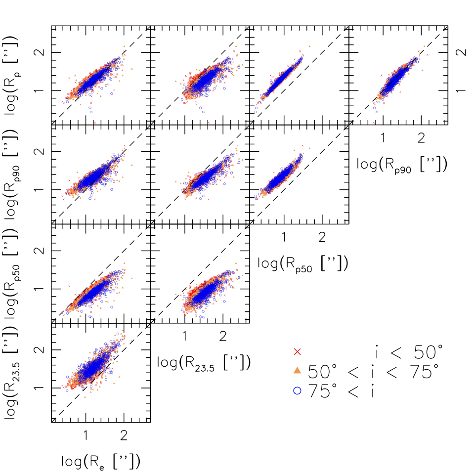


.
