An analysis of mixing angles in presence of New Physics
and an update of
Abstract
We discuss a simple approach to measure the weak mixing angles and of the and systems in the presence of New Physics. We present a new expression that allows one to measure directly if New Physics contributes significantly to the mixing only. We apply the method to specific penguin-mediated , and modes. We provide a very stringent and simple bound on the direct CP asymmetries of all these modes, the violation of which is a signal of New Physics in decay. Within the same theoretical framework, an updated prediction for the branching ratio of is presented, which can be compared with a recent LHCb analysis.
pacs
13.25.Hw, 11.30.Er, 11.30.HvIn our quest for New Physics (NP) in flavour processes, the weak angles involved in the mixing of () and () mesons have been studied with a great attention recently, since they have shown interesting discrepancies with respect to the Standard Model [1, 2]. On the one hand, there is a tension in the SM fit between the measurement of and the branching ratio of (see also Refs. [3, 4] where the discrepancies with respect to other inputs are discussed, e.g., inclusive or exclusive semileptonic decays, or mixing-dependent observables). On the other hand, the most recent angular analyses of by CDF, DØ and LHCb [5, 6, 7] seem to reduce substantially the space for New Physics in . Finally, there still remains an important discrepancy with the Standard Model through the dimuon asymmetry measured at DØ [8, 9].
In this context, it is useful to devise alternative methods to extract the mixing angle of both () and () systems from experiment. In this paper we will take the point of view of assuming that New Physics contributes significantly only to the mixing phases whereas the formalism of the CKM matrix can still be used to analyse decay amplitudes. Under this assumption we present a clean method to extract the NP contribution to the weak mixing phase from selected and decays.
Some time ago [10], we proposed a test on the value of in the SM by measuring certain longitudinal branching ratios and CP asymmetries of mesons decaying into vectors, for modes mediated by penguin diagrams – we focused on the potential of the decay at that time. The method has advantages both from the theoretical and experimental points of view. On the theoretical side, it reduces the required theoretical input mainly to a single hadronic quantity , defined as the difference between “tree” and “penguin” contributions. More precisely, for a meson decaying through a penguin-mediated process, the decomposition
| (1) |
with the CKM factors , can be used to define as the difference of the hadronic matrix elements that are multiplied by and respectively, i.e.,
| (2) |
In the case of penguin-mediated decays, the evaluation of this quantity using QCD factorisation (QCDF) is expected to be particularly robust, as it was built specifically to cancel the infrared divergences coming from spectator-quark and annihilation contributions up to next-to-leading order 11 1 Notice that this cancellation is ensured at NLO in the strong coupling constant, but it has to be proven that this feature remains at higher orders. [11]. On the experimental side, this test of weak mixing angles within the Standard Model can be performed simply by measuring a CP-averaged branching ratio and an untagged rate. This allows us to avoid tagging, although a time-dependent analysis is still required.
In the present article, we extend this approach beyond the simple SM test on the weak mixing angles and presented in Ref. [10]. Indeed, we show that we can also use penguin-mediated decays to measure the size of NP contributions to neutral-meson mixing, assuming that its contribution to decays is negligible. We also update our predictions for the branching ratio of which has been recently measured. The paper is organized in the following way. In Section I, we present a formula to pin down the NP contribution to and , obtained from transitions, under the assumption that NP provides significant contributions only to the meson-mixing phases. In Section II we discuss the main theoretical input in this method. In Section III we consider three different examples of the method, corresponding to and decays. We update our prediction in Ref. [10] for in Section IV, and compare it with its recent measurement by the LHCb collaboration [12]. In Appendix A we provide a dictionary between the experimental measurements [13, 14] and the theoretical quantities [10] defined for longitudinal observables in decays. In Appendix B, we discuss differences in the determination of the branching ratio for neutral mesons for tagged or untagged analyses, highlighting the role played by the width difference (a problem particularly relevant for mesons).
I Formulae for NP mixing angles
Using the unitarity relation , we can write Eq. (1) in terms of and
| (3) |
The weak phase in is the angle , defined as
| (4) |
whereas is real to a very good approximation for both . Following the definitions in Appendix A, we introduce the observables: a branching ratio (where is the phase space factor) and three CP asymmetries , and
| (5) |
defined in terms of and its CP-conjugate , as well as the meson-mixing phase ( is the CP parity of the final state).
These four observables can be written, using Eq. (3), in terms of , , and . One can then eliminate the hadronic parameter to obtain a relationship between these observables
| (6) | |||||
with defined as
| (7) |
being the new physics contribution to the mixing angle of the system: . In deriving Eq. (6) we have assumed that New Physics could alter only the mixing phase of the neutral meson, but not the CKM matrix elements involved in the decay process. Eq. (6) is a generalization of similar formulae developed in Refs. [11, 10] in the context of the SM. This relation is the starting point of our analysis.
Collecting all terms on the left-hand side in Eq. (6), and defining
| (8) |
we can solve Eq. (6) for :
| (9) |
Here, , and , with the relation:
| (10) |
There is a two-fold ambiguity in Eq. (9). In practice, we will see that (or equivalently ), so that the two solutions are very close and they can be considered as one single solution within current theoretical and experimental uncertainties. Notice also that , which provides a very strong and interesting constraint on the size of :
| (11) |
In general, a pair of values for and imply an upper bound on [10, 15] which is much tighter than the experimental value for . A violation of this bound would be an indication of NP in decay. In the following we will take in the numerical analyses. For example, in the case of we have , which implies .
If there is no New Physics and if the process considered is such that , one recovers and , as can be checked from Eq. (7). In this case, Eq. (6) reduces to the simple relation:
| (12) |
This compact equation can be easily rewritten as a SM test of the angles of the unitarity triangle and corresponds to Eqs. (33)-(36) of Ref. [10].
II Theoretical Input
The theoretical input in this formalism is limited to the quantity defined in Eq. (2). As discussed in Refs. [10, 11], this quantity can be computed safely within QCD factorisation for penguin mediated decays because of the cancellation of long-distance contributions. As a consequence of this cancellation, only penguin contractions contribute to , as can be seen by inspection of the formulae in Ref. [16]. The general form of for a decay is [10, 11]:
| (13) |
where picks up the spectator quark of the meson. The normalisation involves the decay constant and a form factor:
| (14) |
is the relevant Wilson coefficient of the effective Hamiltonian at a scale of order . is the penguin function with a or a quark running in the loop and the sign depends on whether is a pseudoscalar or a vector meson (see [16, 17] for the precise definition of the quantities entering ). For identical particles in the final state (for instance ) an extra factor of must be included in .
In the case in which both and are vector mesons, there is a different for each of the three transversity amplitudes. As discussed in Ref. [17], only longitudinal amplitudes can be handled safely within QCD factorisation, so we shall focus on longitudinal polarisations for vector-vector modes, in the spirit of Ref. [10] (see also Ref. [18] for a discussion of transverse amplitudes in QCDF). This requires the definition of suitable longitudinal observables, together with a procedure to extract them from the observables that are actually measured, as discussed in more detail in the appendices of the present article.
In Table 1 we present the values of for penguin-mediated decay channels, with (where stands for longitudinally polarised vectors), using the same hadronic inputs as in Ref. [10].
| Channel | ||
|---|---|---|
III Neutral-meson mixing angles from and
In this section we illustrate the determination of the NP contributions to both weak mixing angles and using Eqs. (6) and (9). We consider channels of three different types: (), (), and (). We will see that in the case of and , all the required observables are already measured, which allows us to perform a complete analysis to extract . There is no experimental data for , so we will only be able to present a case study, which can be exploited immediately as soon as data is available.
Besides the theory input and the measured branching ratio, we need additional inputs for the SM CKM parameters. Since we are assuming that meson mixing could be affected by NP, we must use values of the CKM elements extracted using modes insensitive to mixing. The fit in Table 11 of Ref. [1] satisfies this requirement, as the mixing-related observables included in this fit are used essentially to determine the size of NP in meson mixing and have a very small impact on the CKM parameter themselves, which are thus determined from tree-dominated quantities. Indeed we checked that a fit limited to the tree dominated inputs of Ref. [1] yields almost identical results for the CKM parameters. From Ref. [1] we obtain, upon symmetrizing errors:
| (15) | |||||
which will be used in the following studies.
III.1 First example:
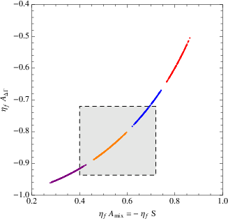
We first consider . Using the formulae in Eq. (9), together with and in Table 1, and the experimental numbers and [19] (the product of intrinsic parities is ), we find the two solutions for the NP contribution to the mixing angle:
| (16) |
from which we can give an averaged result:
| (17) |
This result is (marginally) compatible with the SM value . However the error on is almost completely dominated by the experimental uncertainty in : any improvement on the latter would impact our knowledge of and its agreement with SM expectations.
In Figure 1 we show the regions in the - plane corresponding to different values of , the NP contribution to the mixing angle. The easiest way to understand this plot is through the two constraints on and : Eq. (6) is a linear equation at fixed , whereas
yields a radial constraint. For a fixed , the solution for and is thus given by the intersection of a line with the unit circle. If this line is tangent, the solution is limited to one point, and our determination is perfectly precise. The opposite situation occurs if the line goes through the origin. It turns out that the distance of this line from the origin is given exactly by , so measures the precision with which we can determine :
The smaller the value of , the more precisely we can pin down the value of .
The SM solution is shown explicitly in Fig. 1, and the gray box indicates the current experimental situation. One can see there is marginal agreement, in line with the result in Eq. (17). We stress that these results include all known hadronic uncertainties, and the errors are relatively small because the chosen theoretical input is robust. A more precise value for the angle would achieve a substantial reduction of the regions of fixed in Fig. 1.
It should be mentioned that, since we have no way of determining the sign of , there is a second box in Fig. 1 that has not been drawn, corresponding to . We have discarded this possibility because it leads to a very large New Physics mixing angle.
III.2 Second example:
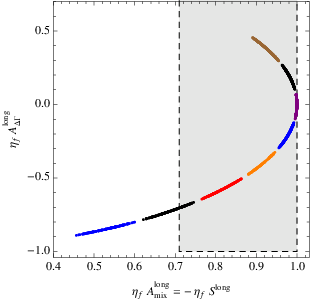
An angular analysis of the decay is available from both Babar and Belle collaborations [13, 14], with an additional time-dependent analysis for the former experiment. The averaged results read [19, 13]
| (18) |
Using equations (50)-(53) in Appendix A (and noting that ), we obtain the longitudinal observables:
| (19) | |||||
Compared to the case of , the uncertainty on is so large that one cannot distinguish, among the two solutions, which one is disfavored by too large a value of the NP mixing angle. For illustration we focus on the negative solution of .
For this decay, Eq. (11) yields the following range for the direct asymmetry:
| (20) |
which is more precise than the experimental value in Eq. (19), and which is used in the following. Equation (9) then yields the two solutions:
| (21) |
which can be averaged as
| (22) |
This result is compatible with the SM (), and also with the result obtained from (Eq. (17)), within large uncertainties.
In Fig. 2, we show the regions in the - plane corresponding to different values of the NP contribution to the mixing angle. The SM solution is shown explicitly, and the gray box indicates the current experimental situation. From this plot we see that a more accurate knowledge of or would be very useful to test the SM hypothesis.
III.3 Third example:
There is currently no information on this mode. However, the U-spin related decay has the measured branching ratio [19]:
| (23) |
As explained in Ref. [11], if there is no NP affecting the decay , one can predict the SM branching ratio for the decay quite precisely. This prediction is not affected by a possible NP contribution to (see Section 3 of Ref. [10]), and since we are assuming that there is no NP affecting processes, it is a good option to take this prediction as an input for our analysis [11]:
| (24) |
The present analysis of this decay should be considered as a case study, waiting for data to be available.
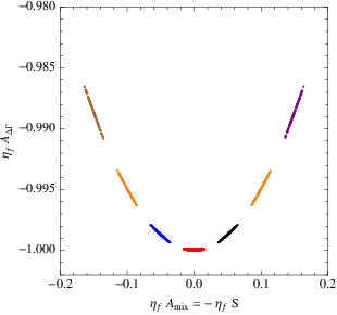
Without further experimental information on CP asymmetries, we cannot use Eq. (9) to extract , the NP contribution to the mixing angle. But it is still possible to determine the regions in the - plane that correspond to each value of , similarly to Figs. 1 and 2. Notice that in the present case we have simply , since here. The case is shown in Figure 3. Whenever the branching ratio for this mode is measured, this plot can be remade, although we do not expect it to change in an appreciable way. A precise measurement of the time-dependent CP asymmetry will then provide an accurate determination of .
One may wonder why we did not consider the decay at a first stage, since its branching ratio is known. However, the prospects for this particular decay are not very alluring. The mixing angle involved in the expression for (Eq. (8)) is , and the branching ratio is not particularly large, so that the value of is small but not tiny (). As mentioned above, the value of determines the potential accuracy of our procedure, which turns out to be rather poor in the present case. This is true in general for all transitions in our list (see Table 1); however, the situation may change if the branching ratio of some of the modes is found to be large enough, as it might be for .
IV The Branching ratios within the SM
In this section, we present a prediction for in the SM using our approach. This prediction can be easily turned, as shown later on, into a prediction for the total branching ratio, once , and are measured (see Appendix A for details). This section is an update of results presented in Ref. [10].
The two decays , with , are related by U-spin symmetry. The symmetry-breaking effects can be separated into a factorizable and a non-factorizable part. This translates into the following relations involving the hadronic parameters and
| (25) |
with the factorisable factor
| (26) |
and account for the non-factorizable symmetry breaking effects. There is no theoretically clean way to compute these quantities. Here we use QCD-factorisation to estimate an upper bound on this corrections. We get , and keep its phase as a free parameter (even though QCD factorisation would predict it to be small). It is very easy to show that the quantity is related to through
| (27) |
Observables related to the decay can be obtained if the ones for are known. An important result discussed in Ref. [10] is that the ratio
| (28) |
is almost a constant if , even in the presence of NP in mixing. Indeed, when the two branching ratios in Eq. (28) are reexpressed in terms of and (as computed in Table 1), it becomes clear that the ratio is completely dominated by the penguin contributions and for large enough , and thus determined by and essentially. This behaviour is confirmed in Table 2 for several values of the branching ratio.
Our result, combining all the error sources, is
| (29) |
which updates Table IV in Ref. [10]. The improvement on the uncertainty comes in particular from Eq. (27) which was not used in this reference. We have added the superscript “DMV” to distinguish our determination from other ones that we will describe now.
Indeed this number can be compared with the value obtained within the QCDF framework taking the usual model for -suppressed corrections described in Ref. [17]. The corresponding predictions are for the decay mode: and , and for the corresponding decay mode: and . We write in terms of total branching ratios and polarisation fractions, as described in Appendix A
| (30) |
where we introduce the correcting factor
| (31) |
In Ref. [17], the predictions within QCDF are and . Since the QCDF predictions are dominated by longitudinal polarisation, we assume and to be of the same size, leading to a factor ranging from 0.98 to 1, and to the QCDF prediction
| (32) |
Alternatively, if data on is used to control annihilation rather than the usual model for these -suppressed corrections, the predictions become [17]: , , and . In this case the prediction is practically the same but with smaller errors:
| (33) |
which is consistent with our result because of the large error bars, even though the central value is a bit low compared to ours.
The most recent experimental values [19] for and are consistent with the QCDF prediction, although both are on the high range. The LHCb collaboration has measured the mode very recently, reporting the following numbers [12]: and .
Following the discussion in Appendix B, we can express the ratio in terms of experimentally measured quantities:
| (34) |
where we define . In both cases, it was assumed in the experimental analysis that there is no -violation in decay, and therefore we do not include the corrections associated with the direct asymmetries. We take [19], and the SM value of . These results imply a quite low value for :
| (35) |
The measured value of is unexpectedly low with respect to the polarisation fraction for the -spin related channel: . If , we would obtain a ratio in better agreement with Eq. (29), although would fit better.
An alternative determination of this branching ratio using data from yields the result [20] in fair agreement with the previous result:
| (36) |
A similar exercise with yields , once again in better agreement with our expectations.
Finally, one can invert these relations and get a prediction for the total , as measured at a hadronic machine (thereby the subscript ‘LHCb’):
which can be trivially updated if the longitudinal polarisation of the mode changes.
We remind the reader that, as opposed to the rest of the paper, all the predictions in this section have been obtained within the SM. A detailed analysis of the impact of NP on these observables is certainly worthwhile, but lies beyond the scope of the present article.
CONCLUSIONS
We have shown how to exploit and penguin-mediated decays in order to obtain the New Physics contribution to the weak mixing phase of both and systems, under the assumption of no significant New Physics contribution to the decay amplitudes. The main theoretical input consists of the infrared-safe quantity , which can be evaluated within QCD factorisation with a good theoretical control. It is interesting that the experimental knowledge of the branching ratio by itself yields a stringent bound on the direct CP asymmetry, Eq. (11). As a consequence, the knowledge of BR and is sufficient to determine the New Physics contribution to the weak mixing angles. Different examples are discussed and the corresponding values for presented; however, more precise data is required before a clear conclusion can be reached.
These results should be compared with the one obtained from charmonium modes, where one is also sensitive to the NP mixing angle. Time-dependent analyses of give the average [1, 19]: . Using the value quoted in Eq. (15) for the SM contribution leads to the estimate
| (38) |
In Ref. [1], the analysis of NP contributions to both and mixings (so-called scenario I) including the experimental information available at that time led to the following value for the NP mixing phase in the sector
| (39) |
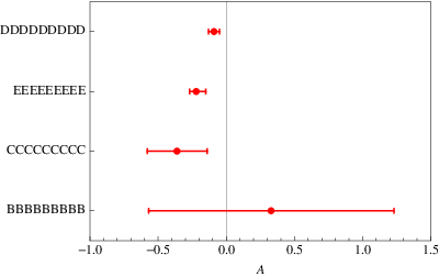
The main ingredient for this value is the discrepancy between and in the SM, and thus it will only be marginally affected by the CDF, DØ and LHCb updates concerning the sector. The comparison of these numbers with the ones obtained in Section III is shown in Fig. 4.
Finally, an updated result for the longitudinal observables of the decay mode has been presented. For the ratio of to longitudinal branching ratios, defined in Eq. (28), we find:
| (40) |
This result can be compared with recent experimental analyses, and with similar theoretical predictions obtained with alternative approaches:
- 1.
Our result is compatible with the QCDF prediction (see Eq. (32)), although our error is about four times smaller. If the QCDF is supplemented with data to fix -suppressed corrections of phenomenological relevance, the error decreases, but still is twice as large as ours.
- 2.
Our result is compatible with the recent LHCb measurement, Eq (35), although the experimental number seems rather low. We tentatively identify this anomaly with the surprisingly low value for the longitudinal polarisation fraction : a value of , similar to the one measured for the -spin related mode, would lead to a , more in agreement with our prediction. If the LHCb measurement of is confirmed, its interpretation would constitute a theoretical challenge, as it would require a type of NP that violates the flavour symmetry relating and decays very significantly.
We hope that these results will trigger more precise experimental analyses of penguin-mediated decays both in and sectors, considering the potential of these channels to identify New Physics in meson mixing.
Acknowledgements.
We would like to thank B. Adeva for discussions and comments. J.V. is supported in part by ICREA-Academia funds. J.M. acknowledges financial support from FPA2008-01430, SGR2009-00894.Appendix A Dictionary for longitudinal observables in decays
In the case of two-body decays into vector mesons and , there are three different configurations of helicity available . This is described by three transversity amplitudes corresponding to linearly polarised states, with definite CP properties ( correspond to a -parity , whereas has ). As discussed extensively in Ref. [18, 17], the transversal amplitudes are suppressed by powers of compared to the longitudinal amplitude , leading to an expected longitudinal polarisation close to 1. In turn, this implies that predictions based on the heavy-quark limit, such as those from QCD factorisation or SCET, are much more reliable for longitunal observables than for parallel and perpendicular ones, where only rough estimates can be derived.
This theoretical situation explains why we considered only longitudinal observables for modes in Ref. [10] as well as in the present article. We defined longitudinal observables as the CP observables constructed by considering as final CP eigenstate the two-meson state with longitudinal polarisations, i.e., the CP-averaged branching ratio and the CP-asymmetries
| (41) | |||||
| (42) | |||||
| (43) |
with the phase space factor relating an amplitude to the corresponding branching ratio
| (44) |
represents the longitudinal decay amplitude for , its CP conjugate, and the meson-mixing angle.
In principle, these quantities can be obtained from the angular analysis of the differential decay width (with respect to the usual angular variables [17])
| (45) |
If the initial meson is charged, or if we neglect the difference of lifetimes between neutral mesons (), the coefficients and the transversity amplitudes can be identified up to a global normalisation factor, and the quantities (41)-(43) are easy to obtain from an angular analysis of the decay, as explained in the following.
For the moment, the only available detailed time-dependent analyses for modes of interest to us concerns [13, 14], providing CP-averaged parameters and CP-asymmetries for the 3 transversity amplitudes (these analyses for the meson set ). Using a superscript for observables and a superscript for observables, one has values for the branching ratios
| (46) | |||||
| (47) |
and for the polarisation fractions
| (48) |
We have therefore the relationships
| (49) |
and we can easily define the longitudinal observables in terms of these observables
| (50) | |||
| (51) | |||
| (52) | |||
| (53) |
where the relative phase between and is defined following the notation of Ref. [13]
| (54) |
In this analysis, the mixing angle was assumed to have its Standard Model value rad, which we used to translate the measured quantities into the longitudinal observables and . In the experimental analysis of Ref. [13], there is only sensitivity to , which means that there is a sign ambiguity in , as seen in Eq. (19).
Appendix B Neutral-meson observables with a finite width difference
Since we consider the meson in the present article, we have to discuss the modifications induced by a finite lifetime difference, before distinguishing its impact on flavour-tagged and flavour-untagged analyses for the longitudinal observables of interest. We will see that we must include different corrections in each case to connect the measured quantities and the observables (41)-(43). As will become clear in the following, most of this discussion applies not only to two-body vector modes but more generally to any decay of a neutral meson into a eigenstate.
B.1 Branching ratios in presence of meson mixing
The - systems can be described in terms of CP-conjugate flavour states and (). The time evolution of an isolated neutral meson of a given flavour at and decaying at a later time into a CP eigenstate is given as [22, 21]
| (55) | |||
| (56) |
where the Hamitonian eigenvalues define . Also, and . is a time-independent, but state-dependent normalisation factor, corresponding to the integration over phase space. The mixing ratio is assumed to be a pure phase in the present article (as suggested by the very small values of the flavour specific asymmetries both for and [19]).
The normalisation factor comes from
| (57) |
Let us notice that this “definition” is rather ambiguous, as one generally considers initial and final states that are asymptotic (mass eigen)states, which is not. However, one can still determine this factor by going back to the derivation of Fermi’s golden rule. This is generally done for an initial mass eigenstate of the unperturbed Hamiltonian but can be easily adapted to the superposition of two mass eigenstates , provided that the difference of energy between the two transitions is small. In that case, the normalisation corresponds to the phase space available, computed for the mass eigenstates of the unperturbed Hamiltonian. We obtain therefore the same normalisation as in the case of charged -decays
| (58) |
where is given by the phase space with an incoming meson of mass .
Since there is no unambiguous definition of the CP-averaged branching ratio for neutral mesons as the states involved ( and ) are not mass eigenstates, we should define what we call the CP-averaged branching ratio for decays. We opt for the simple definition, inspired by the charged meson case, and corresponding to the value that we would obtain through a measurement at (i.e., before neutral -meson mixing could take place)
| (59) |
We will show later that this definition coincides exactly with time-integrated CP-averaged decay widths in the limit , but that the relationship is corrected by terms of order . This correction depends on the experimental setting, because each one has a different sensitivity to the time evolution of the neutral -meson. This correction factor can thus be seen as a correction for the temporal acceptance of the considered experiment.
Let us now come to decays, and let us assume that all the direct asymmetries vanish, whereas and , where . As discussed in Ref. [21], we can obtain the time-dependent decay width from Eq. (45), upon the identification
| (60) | |||
| (61) | |||
| (62) | |||
with , and and the relative strong phases of and with respect to . There is a common normalisation factor for all amplitudes. The CP-conjugate expression can be obtained by the replacement and by multiplying by the two imaginary parts involving in Eq. (62).
B.2 Tagged analysis
Flavour-tagged analyses are particularly easy to perform in -factories as they produce intricated pairs [13], and they allow one to study separately the time-dependence of and samples as well as to extract the modulus and relative phases of the three transversity amplitudes through an angular analysis. The probability of the process depends on the decay times and of both mesons (the one decaying into a tagging state and the one actually studied for CP-violation and decaying into ). After integrating over the sum , one obtains for a structure similar to that for untagged decays provided that the exponential is replaced by and that is allowed to run from to . Indeed, from Ch. 1 in Ref. [23], we have the joint decay amplitude which can be integrated over time to yield
| (63) | |||
where the first factor comes from the angular integral describing the transition, and we have defined as the integrand of Eq. (63).
In the case of a non-vanishing width difference, and assuming the normalisation Eq. (59), we can determine the CP-averaged branching ratio by considering
| (64) | |||||
We have therefore a correction of the time-integrated branching ratio with respect to the branching ratio in absence of mixing. This correction is due to the difference of the widths between the two neutral states. This is typically a small correction: if we define , we can write [19]
| (65) |
B.3 Untagged analysis
In the case of hadronic machines, such as CDF, D0 and LHCb, we encounter a rather different situation with no flavour tags available and an integral over time being performed. Since there is no information on the second -meson being produced, one must consider Eqs. (55) and (56) for . The CP-averaged branching ratio can then be determined through
| (66) | |||||
Compared to the tagged case, we see that there is a further term coming from . The resulting correction for the branching ratio is larger than the one for B-factories, since it is linear in the small quantity , and not quadratic.
For vector-vector channels, assuming that the production rate for and is the same and that there is no CP-violation in decay, yields an angular structure identical to Eq. (45), with the replacement
| (67) | |||||
| (68) | |||||
| (69) | |||||
where the terms are the remnants of . After integration over the angles, we obtain the CP-averaged width
| (70) |
which is expressed in terms of the longitudinal and transverse CP-averaged branching ratios.
In the case of the LHCb analysis for (), an angular analysis was performed to extract the total branching ratio as well as the longitudinal polarisation. The expression in Ref. [7] for the latter quantity was given in the SM case with a vanishing mixing angle . However, the angular analysis performed does not rely on this assumption, so that we can just identify the coefficients with the same angular dependence in the differential decay width, leading to: . We can thus derive the relation, valid in the absence of CP-violation in decay
| (71) |
We see that even in the SM case where is tiny, there is a small contribution from to the relationship between the polarisation measured at LHCb and .
References
- [1] A. Lenz, U. Nierste, J. Charles, S. Descotes-Genon, A. Jantsch, C. Kaufhold, H. Lacker, S. Monteil et al., Phys. Rev. D83, 036004 (2011).
- [2] J. Charles, O. Deschamps, S. Descotes-Genon, R. Itoh, H. Lacker, A. Menzel, S. Monteil, V. Niess et al., Phys. Rev. D84 (2011) 033005.
- [3] E. Lunghi, A. Soni, Phys. Lett. B697, 323-328 (2011).
- [4] R. Barbieri, P. Campli, G. Isidori, F. Sala, D. M. Straub, [arXiv:1108.5125 [hep-ph]].
- [5] CDF Collaboration, CDF Note 10206, November 2, 2010, http://www-cdf.fnal.gov/ physics/new/bottom/100513. blessed-BsJpsiPhi 5.2fb/cdf10206 sin2betas.pdf
- [6] S. Burdin [D0 Collaboration], “Measurements of CP violation in the Bs system at D0”, talk given at the Europhysics Conference on High-Energy Physics 2011, July 21 2011. http://indico.in2p3.fr/getFile.py/access?con tribId=1005&sessionId=2&resId=0&materialId=slides& confId=5116
- [7] LHCb Collaboration, LHCb-CONF-2011-049.
- [8] V. M. Abazov et al. [D0 Collaboration], Phys. Rev. D82, 032001 (2010).
- [9] V. M. Abazov et al. [D0 Collaboration], Phys. Rev. Lett. 105, 081801 (2010).
- [10] S. Descotes-Genon, J. Matias and J. Virto, Phys. Rev. D 76 (2007) 074005.
- [11] S. Descotes-Genon, J. Matias and J. Virto, Phys. Rev. Lett. 97, 061801 (2006).
- [12] R. Aaij et al. [LHCb Collaboration], arXiv:1111.4183.
- [13] B. Aubert et al. [BABAR Collaboration], Phys. Rev. D 78, 092008 (2008).
- [14] K. F. Chen et al. [BELLE Collaboration], Phys. Rev. Lett. 94, 221804 (2005).
- [15] J. Virto, AIP Conf. Proc. 964, 90-94 (2007).
- [16] M. Beneke and M. Neubert, Nucl.Phys.B 675 (2003) 333.
- [17] M. Beneke, J. Rohrer and D. Yang, Nucl. Phys. B774, 64-101 (2007).
- [18] A. L. Kagan, Phys. Lett. B601, 151-163 (2004).
- [19] Heavy Flavor Averaging Group (HFAG), http://www. slac.stanford.edu/xorg/hfag/.
- [20] LHCb Collaboration, note LHCb-CONF-2011-019.
- [21] I. Dunietz, R. Fleischer and U. Nierste, Phys. Rev. D 63 (2001) 114015.
- [22] I. Dunietz, J. L. Rosner, Phys. Rev. D 34 (1986) 1404.
- [23] P. F. Harrison and H. R. Quinn Eds. “The BABAR physics book: Physics at an asymmetric B-factory”.