Toward Spin Squeezing with Trapped Ions

Exploitation of coherent quantum phenomena represents a new frontier in the field of metrology, that study which aims to achieve measurements of physical phenomena with ever increasing precision. Probably the prototypical quantum metrology experiment is the simple Ramsey interferometry measurement used in atomic clocks, which for decades has been the basis for the calibration of time and frequency standards. Modern quantum metrology experiments, however, often entail sophisticated manipulation of several quantum degrees of freedom to achieve a single measurement outcome. As an example consider the quantum-logic spectroscopy clock measurements in which the state of an internal clock transition of one atom is transferred to a detectable transition in an auxiliary atom using the quantum mechanical motion of the atoms as a bus [1].

A natural limit in precision of a measurement carried out on an ensemble of $N$ uncorrelated particles is the standard quantum limit, in which the measurement precision scales with $\sim 1/\sqrt{N}$. This scaling is a direct consequence of the Poissonnian statistics resulting from the lack of correlation between the measurement outcomes of the individual particles. On the other hand, the intrinsic limit of a quantum measurement is governed by Heisenberg’s uncertainty principle and allows the precision to scale as $\sim 1/N$, the Heisenberg limit [2]. Any quantum state that allows a measurement precision surpassing the standard quantum limit is said to be “squeezed”. This proceedings reviews the mathematical description of squeezing in pseudo-spin systems and current progress toward implementing squeezing in trapped ion systems.

Several strategies to achieve spin squeezing exist, and a number have been implemented experimentally. One method is through the use of quantum non-demolition measurements. A typical implementation relies on the coupling between the Stokes vector of a probe beam of light and the spin state of an ensemble of cold atoms. This coupling induces a spin-dependent polarization rotation of the probe beam, which can be measured with a polarimeter down-stream of the atoms. The outcome of such a measurement allows one to improve one’s prediction for the outcome of a subsequent measurement, which constitutes a reduction in spin noise, i.e. squeezing of the spin uncertainty. Although this measurement conveys information regarding the spin-state it is non-projective and hence is labelled as a non-demolition measurement. Oftentimes the amount of squeezing is characterized by comparing the ratio of the variances of the measured spin component of the squeezed versus unsqueezed states:

$$\mathcal{S}=10\log{\left(\frac{\sigma^{2}_{squeeze}}{\sigma^{2}_{unsqueeze}}\right)}.$$

(1)

This approach has been used by Appel et al. [3] as well as Takano et al. [4] to produce respectively $\mathcal{S}=-3.4$ dB and $\mathcal{S}=-1.8$ dB of squeezing.

An alternative approach to squeezing is through engineering of a phase shift that depends nonlinearly on the spin-state of the particles. In cold, neutral atomic gases one way to realize such a nonlinearity is via the mean-field interaction resulting from interparticle s-wave scattering. This interaction is ever-present, so the technical challenge is to turn it on, or off, controllably. This ability was recently demonstrated by two groups. Riedel et al. [5] studied a two-component Bose-Einstein condensate formed by atoms in different hyperfine states. They controlled the nonlinearity by employing a trap which can indepently manipulate the trapping potential of the two components. Since the mean-field interaction depends on the overlap of the wavefunctions of the two components, which their trap allowed them to vary, they were able to controllably squeeze and achieve a reduction in spin noise of $\mathcal{S}=-3.7$ dB. Gross and co-workers [6] achieved the same goal by instead tuning the s-wave scattering length using a narrow Feschbach resonance, obtaining $\mathcal{S}=-8.2$ dB of squeezing.

A nonlinearity can also be engineered by placing an ensemble of atoms in an optical cavity. The presence of light circulating in such a cavity induces an ac Stark shift on the hyperfine groundstate levels close to resonance with the cavity mode. The atoms in turn modify the index of refraction in the cavity which shifts the cavity resonance frequency. As a result, the light shift on each atom depends on the presence of all other atoms in the cavity leading to the nonlinear phase shift required for squeezing. Leroux and others [7] achieved $\mathcal{S}=-5.6$dB of squeezing using this approach. Recently, using a similar approach Thompson and co-workers achieved $\mathcal{S}=-3.4$ dB of squeezing on nearly $10^{6}$ Rb atoms [8].

The aim of this proceedings is to give a pedagogic overview of the formalism needed to describe squeezing in an ensemble of two-level systems, as well as the quantum optics relevant to a particular implementation using trapped ions in a Penning trap that depends on creation of a nonlinear phase shift. The rest of this manuscript is organized as follows: in the next section we summarize the mathematical language required to describe the squeezing effect in an ensemble of two-level particles. We then consider the spin squeezing interaction first discussed in detail by Kitagawa and Ueda [9]. This is followed by a description of how the squeezing interaction can be engineered in a trapped ion system, which builds on the first squeezing demonstrations with two trapped ions in a radio-frequency Paul trap [10]. The particulars of the Penning ion trap experiment are then discussed before the final section looks at some of the technical challenges faced in successfully implementing the experiment.

In this section we develop a convenient mathematical description for an ensemble of $N$ two-level systems of which the two levels are coupled by an oscillating electric or magnetic field. Assuming each particle can be in either of the states $|\!\downarrow\rangle$, $|\!\uparrow\rangle$, the many particle Hamiltonian coupling the two states can be expressed in a frame rotating at the transition frequency between the levels as

$$H=\sum\limits_{i=1}^{N}\frac{\hbar}{2}\delta\sigma^{z}_{i}+\hbar\Omega_{R}\sum\limits_{i=1}^{N}\left(\sigma_{i}^{-}+\sigma_{i}^{+}\right),$$

(2)

where the index $i$ labels the $i$’th particle. Here $\delta=\omega_{0}-\omega$ is the detuning between the transition frequency $\omega_{0}$ and drive field frequency $\omega$, $\sigma^{z}_{i}$ is the Pauli operator, obeying the usual spin angular momentum commutation relation $\left[\sigma^{x}_{i},\sigma^{y}_{i}\right]=2i\varepsilon_{xyz}\sigma^{z}_{i}$, while the raising and lowering operators are defined via $\sigma_{i}^{+}=\frac{1}{2}(\sigma_{i}^{x}+i\sigma_{i}^{y})$, $\sigma_{i}^{-}=\frac{1}{2}(\sigma_{i}^{x}-i\sigma_{i}^{y})$ and have the effects: $\sigma^{+}_{i}|\!\downarrow\rangle=|\!\uparrow\rangle$, $\sigma^{-}_{i}|\!\uparrow\rangle=|\!\downarrow\rangle$. It is convenient to introduce the following pseudo-spin operators

$$J_{z}=\sum\limits_{i}\frac{1}{2}\sigma^{z}_{i},\hskip 28.45274ptJ_{+}=\sum\limits_{i}\sigma^{+}_{i},\hskip 28.45274ptJ_{-}=\sum\limits_{i}\sigma^{-}_{i}.$$

(3)

This transformation preserves the spin commutator relation $\left[J_{x},J_{y}\right]=2i\varepsilon_{xyz}J_{z}$ and allows the the Hamiltonian to be written concisely as

$$H=\hbar\delta J^{z}+\hbar\Omega_{R}\left(J^{-}+J^{+}\right).$$

(4)

As typical experiments are initiated with all particles optically pumped to a specific state, we consider the action of the lowering operator on that initial state with all particles in $|\!\uparrow\rangle$, i.e. $|J=N/2,M_{J}=N/2\rangle=|N/2,N/2\rangle=|\uparrow\uparrow\uparrow...\uparrow\uparrow\rangle$. The choice of labelling in the left-hand ket in the latter will become clear presently. Operating consecutively with the lowering operator we get (the normalization factors in what follows are explicitly calculated in Appendix A):

	$\displaystyle\hskip-34.14322pt|N/2,N/2-1\rangle=\frac{1}{\sqrt{N}}J_{-}|\uparrow\uparrow\uparrow...\uparrow\uparrow\rangle=\sum\limits_{j}\frac{\sigma^{-}_{j}}{\sqrt{N}}|\uparrow\uparrow\uparrow...\uparrow\uparrow\rangle=\frac{1}{\sqrt{N}}\sum\limits_{j}|\uparrow\uparrow...\downarrow_{j}...\uparrow\uparrow\rangle$		(5)
	$\displaystyle\hskip-34.14322pt|N/2,N/2-2\rangle=\frac{1}{\sqrt{2!N(N-1)}}J_{-}^{2}|\uparrow\uparrow\uparrow...\uparrow\uparrow\rangle$		(6)
	$\displaystyle\hskip 39.83368pt=\frac{1}{\sqrt{2!N(N-1)}}\sum\limits_{j_{1},j_{2}}\sigma^{-}_{j_{1}}\sigma^{-}_{j_{2}}|\uparrow\uparrow\uparrow...\uparrow\uparrow\rangle$		(7)
	$\displaystyle\hskip 39.83368pt=\frac{\sqrt{2!}}{\sqrt{N(N-1)}}\sum\limits_{j_{1}<j_{2}}|\uparrow\uparrow...\downarrow_{j_{1}}...\downarrow_{j_{2}}\uparrow\rangle$		(8)

The state on the right hand side in (8) is therefore a symmetric superposition of all number states for which two particles are in the down state and all other particles in the up state. Likewise after applying $J_{-}$ for $N/2$ times, one gets

	$\displaystyle|N/2,0\rangle\!\!\!\!\!$	$\displaystyle=$	$\displaystyle\!\!\!\!\!\frac{1}{\sqrt{N!}}J_{-}^{N/2}|\uparrow\uparrow\uparrow...\uparrow\uparrow\rangle$		(9)
		$\displaystyle=$	$\displaystyle\!\!\!\!\!\frac{1}{\sqrt{N!}}\sum\limits_{j_{1},j_{2},...j_{N/2}}\sigma^{-}_{j_{1}}\sigma^{-}_{j_{2}}...\sigma^{-}_{j_{N/2}}|\uparrow\uparrow\uparrow...\uparrow\uparrow\rangle$		(10)
		$\displaystyle=$	$\displaystyle\!\!\!\!\!\frac{(N/2)!}{\sqrt{N!}}\sum\limits_{j_{1}<j_{2}<...<j_{N/2}}|\uparrow...\downarrow_{j_{1}}..\downarrow_{j_{2}}...\downarrow_{j_{N/2}}..\uparrow\rangle,$		(11)

and $N$ times

$$|N/2,-N/2\rangle=J_{-}^{N}|\uparrow\uparrow\uparrow...\uparrow\uparrow\rangle=|\downarrow\downarrow\downarrow...\downarrow\downarrow\rangle.$$

(12)

Or in general

$$|N/2,N/2-q\rangle=\frac{\sqrt{q!(N-q)!}}{\sqrt{N!}}\sum\limits_{j_{1}<j_{2}<...<j_{q}}|\uparrow...\downarrow_{j_{1}}..\downarrow_{j_{2}}...\downarrow_{j_{q}}..\uparrow\rangle.$$

(13)

It is now apparent that the second index in our labelling of the left-hand kets indicates one-half of the difference between the number of particles in the state $|\!\uparrow\rangle$ versus $|\!\downarrow\rangle$. That number is exactly the eigenvalue of the $J_{z}$ operator, as is clear from the following examples:

	$\displaystyle\hskip-22.76228ptJ_{z}|\uparrow\uparrow\uparrow...\uparrow\uparrow\rangle=\sum\limits_{i}\frac{1}{2}\sigma^{z}_{i}|\uparrow\uparrow\uparrow...\uparrow\uparrow\rangle=\frac{N}{2}|\uparrow\uparrow\uparrow...\uparrow\uparrow\rangle$		(14)
	$\displaystyle\hskip-22.76228ptJ_{z}(\frac{1}{\sqrt{N}}J_{-}|\uparrow\uparrow\uparrow...\uparrow\uparrow\rangle)=\frac{1}{\sqrt{N}}\sum\limits_{i,j}\frac{1}{2}\sigma^{z}_{i}|\uparrow\uparrow...\downarrow_{j}..\uparrow\uparrow\rangle$		(15)
	$\displaystyle\hskip-22.76228pt\hskip 110.96556pt=(\frac{N}{2}-1)\frac{1}{\sqrt{N}}\sum\limits_{i}|\uparrow\uparrow..\downarrow_{i}...\uparrow\uparrow\rangle$		(16)
	$\displaystyle\hskip-22.76228ptJ_{z}\frac{1}{\sqrt{2!N(N-1)}}J_{-}^{2}|\uparrow\uparrow...\uparrow\uparrow\rangle=(\frac{N}{2}-2)\frac{1}{\sqrt{2!N(N-1)}}\sum\limits_{j_{1}\neq j_{2}}|\uparrow...\downarrow_{j_{1}}...\downarrow_{j_{2}}\uparrow\rangle.$		(17)

We have thus constructed a set of basis states that are eigenstates of the $J_{z}$ operator, i.e. $J_{z}|N/2,N/2-m\rangle=(N/2-m)|N/2,N/2-m\rangle$ with $m=0,1,2,...N$. With some more algebra it can be shown that these states are simultaneously eigenstates of the operator $J^{2}=J^{2}_{x}+J^{2}_{y}+J^{2}_{z}$, with the degenerate eigenvalue $(N/2)(N/2+1)$. This motivates the choice of labelling for the first index. The set of states $|N/2,N/2-m\rangle$ therefore behave as eigenstates of a spin angular momentum with magnitude $N/2$, and can be denoted as $|J,M_{J}\rangle$. We will refer to these as a pseudo-spin. These states are well known from the theory of superradiance described by Dicke in 1954 [11] and are often referred to as Dicke states. It is important to note that the states do not span the entire Hilbert space, but just the particular symmetric subspace constructed here. However, since we will consider only experiments initiated with all particles pumped into the state $|\!\uparrow\rangle$, the dynamics accessible through (4) restricts the system to this symmetric subspace.

A useful pictorial description of a single two-level system can be brought to bear here, namely the concept of a Bloch vector. Any state of a single two-level system can be represented by the state vector with coefficients $(e^{-i\phi}\cos{\theta},e^{i\phi}\sin{\theta})$. One can think of the parameters as being the polar angle, $\theta$, and the azimuthal angle, $\phi$, of a unit vector in 3D space, called the Bloch vector as shown in figure 1. Likewise, we can represent the state of the $N$-particle system by a vector of length $N/2$. In analogy to the single particle case, when the Bloch vector points along the positive $z$-axis it represents a state with all particles in $|\!\uparrow\rangle$, when it points along the negative $z$-axis it represents a state with all particles in $|\!\downarrow\rangle$. As a result of the uncertainty relation $\Delta J_{x}\Delta J_{y}\geq\langle J_{z}/4\rangle$ the projections of the Bloch vector onto the $x$ and $y$ axis when in the state $|N/2,N/2\rangle$ are non-zero, so that the vector should instead of a line element, be thought of as a cone with its apex at the origin, and the width of which indicates the uncertainty in the projections.

To complete the picture for other directions on the Bloch sphere we have to consider the dynamics due to (4), which for $\delta=0$ can be simply rewritten as $H=\hbar\Omega_{R}\hat{J}_{x}$. The time evolution then becomes $U(t)=\exp{(-i\Omega_{R}\hat{J}_{x}t)}$ which one recognizes as the rotation operator for the pseudo-spin which causes a rotation of the vector through an angle $\Omega_{R}t$ around the $x$-axis. Starting with the state $|N/2,N/2\rangle$ and operating with $\hat{U}(\Omega_{R}t=\pi/2)$ therefore places the Bloch vector along the $y$-axis. By expanding the $\hat{U}(\pi/2)$ one finds that the state of the system is

$$|CS\rangle=\frac{1}{2^{N/2}}\sum\limits_{M_{J}=-N/2}^{N/2}\begin{pmatrix}N\\ N/2+M_{J}\end{pmatrix}^{1/2}|N/2,M_{J}\rangle$$

(18)

which is known as a coherent spin state. The uncertainty in a measurement of $\langle CS|J_{z}|CS\rangle$ scales as $1/\sqrt{N}$, i.e. the standard quantum limit, due to the binomial distribution of amplitudes in (18).

In a seminal paper in 1993 [9] Kitagawa and Ueda described spin-squeezing in pseudo-spin systems which results from unitary transformations of the form

$$\hat{U}_{Sq}(t)=\exp{\left[-i\chi\hat{J}^{2}_{z}t\right]}.$$

(19)

The effect of the squeezing operator $\hat{U}_{Sq}(t)$ on any superposition of spin states is to induce a phase shift that depends nonlinearly on the $\hat{J}_{z}$ eigenvalue of each state. We consider now the resulting dynamics on the coherent state $|CS\rangle$ defined above. Figure shows a sequence of snapshots of the uncertainty distribution of $|CS\rangle$ for $J=25$ after it has been subjected to $\hat{U}_{Sq}(t)$ for times (a) $\chi t=0$, (b) $\chi t=0.05$ and (c) $\chi t=0.1$ respectively. As a measure of that uncertainty figure plots the modulus squared of the projection of the state $\hat{U}_{Sq}(t)|CS\rangle$ onto a rotated coherent state, $\exp(-i\phi\hat{J}_{z})\exp(-i\theta\hat{J}_{x})|CS\rangle$, as a function of the two rotation angles. It is clear that the squeezing operator shears the uncertainty cone, reducing the uncertainty along one spin axis at the cost of increasing the uncertainty along an orthogonal axis. The state is said to now be “squeezed”. Kitegawa and Ueda referred to this effect as one-axis twisting of the uncertainty cone. Note that as the squeezing takes place, the Bloch vector also shortens even though the system remains in a pure state. An appropriate parameter to quantify the metrologically relevant squeezing, which takes into account this shortening, is $\xi=\Delta J_{\perp}/\sqrt{J/2}$ where $\Delta J_{\perp}$ is the root-mean-squared deviation along the direction of minimum uncertainty. Figure 3 plots $\xi$ as a function of the time that the squeezing operator is applied, again for $J=25$. The squeezing does not indefinitely reduce the uncertainty in $J_{z}$, but eventually reaches a minimum uncertainty around $\xi=0.28$ for $J=25$. The minimum value of $\xi$ decreases for larger numbers of spins as the curvature of the Bloch sphere becomes less [9].

It is this single-axis twisting Hamiltonian that we aim to realize by use of trapped ions, as discussed next.

One way of implementing the squeezing operator (19) in trapped ions relies on a generalization of the geometric ion-qubit phase gate demonstrated by Leibfried et al. [12]. In that experiment the quantum motion of ions in a trap is used as a bus to mediate the nonlinear phase shift required to affect squeezing. An experimental sequence is as follows:
(1) $N$ ions are trapped and cooled in an ion trap with characteristic center-of-mass frequency $\omega_{z}$.
(2) The internal state of the ions is prepared in the superposition $|CS\rangle$, (18).
(3) An oscillatory force is applied to the ions, close to resonance with the axial center-of-mass mode of motion of the multi-ion system. The force is designed to be state dependent, so that ions in the state $|\!\downarrow\rangle$ feel an equal but opposite force to ions in the state $|\!\uparrow\rangle$. As a result the force will depend on the value of $M_{J}$ of the pseudo-spin states.
(4) The frequency of the oscillatory force is chosen off-resonant by a detuning $\delta^{\prime}$, so that after a period $t=2\pi/\delta^{\prime}$ the drive force has completely dephased and rephased with the oscillating ions, thus accelerating and decelerating it and returning it to its initial motional state.

A geometric interpretation gives a simple physical picture of how this sequence leads to squeezing [12]. Since the ions return to their initial motional state, they trace out a closed loop in phase-space, as pictorially represented in Fig. 4. As a result, they acquire a geometric phase, $\Phi$, proportional to the area, $A$, of the loop. Since the force, $F$, on each ion depends on the internal state of that ion, the force on the multi-ion system depends on the difference between the number of ions in the states $|\!\downarrow\rangle$ and $|\!\uparrow\rangle$, and therefore on the eigenvalue of $J_{z}$ for a state $|N/2,N/2-m\rangle$. In turn the radius, $R$ of the phase-space loop depends linearly on the force so that $R\propto F$. Since the area $A=\pi R^{2}$ we therefore know that the $\Phi\propto A\propto J_{z}^{2}$. This relation is precisely what is needed to implement (19).

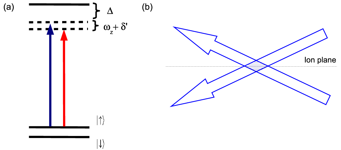
Experimentally the required force is implemented by use of a pair of detuned laser beams illuminating the ions. Consider an ensemble of ions all lying in a single plane, each with a three-level internal structure, as shown in Fig. 5(a). The ions are illuminated by the laser beams in a configuration shown in Fig. 5(b) and the laser beams have frequencies, $\omega_{1}$ and $\omega_{2}$. We require that $\delta^{\prime}\ll\omega_{z}\ll\Delta$. If $\delta_{L}=\omega_{1}-\omega_{2}=0$ the overlapping light fields will form a standing-wave interference pattern along the direction normal to the plane of the ions. The standing wave leads to a position dependent AC Stark shift on the ions, while the gradient of this shift results in a position-dependent force on the ions. Through appropriate choice of laser polarization and detuning, $\Delta$, a different AC Stark shift is obtained for the $|\!\downarrow\rangle$ and $|\!\uparrow\rangle$ states, resulting in a state-dependent force. Detuning the light beams by $\delta_{L}=\omega_{z}$ will cause the standing wave to “walk”, resulting at any point in a periodic force, oscillating at the characteristic center-of-mass frequency of the trap, which will excite the motion of the ions.

A key requirement to ensure that the motion gets excited is that the spatial extent of the ions’ wavefunction is significantly smaller than the wavelength of the standing wave. This condition is referred to as the Lamb-Dicke criterion and can be expressed as $\eta=x_{0}k_{eff}\ll 1$, where $x_{0}$ is the characteristic width of the ions’ spatial wavefunction along $\mathbf{k}_{eff}$, the wavevector of the standing wave. If the Lamb-Dicke criterion is not met, the ion wavefunction will feel a drive force in one direction at some points and in the opposite direction at others. The force will average to zero and no excitation will occur.

Given that the Lamb-Dicke criterion is fulfilled and $\delta_{L}=\omega_{z}+\delta^{\prime}$, one can write down an effective Hamiltonian for the interaction between the light fields and the atom as follows:

$$H=\frac{g^{2}\eta}{\Delta}(\hat{a}^{\dagger}e^{i\delta^{\prime}t}+\hat{a}e^{-i\delta^{\prime}t})J_{z}.$$

(20)

Here $g=dE$ where $d$ is the dipole matrix element and $E$ the amplitude of the light field.

Under the action of Hamiltonian (20) for a time $2\pi/\delta^{\prime}$ the ions will trace out precisely the closed loop in phase space discussed above. This is illustrated in figure 6, where in (a) we plot the average number of excitations of the center-of-mass oscillator mode, $\langle\hat{n}\rangle=\langle\hat{a}^{\dagger}\hat{a}\rangle$, as a function of the time and for different initial states: thick solid line - $|0\rangle|M_{J}=1\rangle$, thin solid line - $|0\rangle|M_{J}=2\rangle$, dashed line - $|0\rangle|M_{J}=3\rangle$, dot-dashed line - $|0\rangle|M_{J}=4\rangle$ and dotted line - $|0\rangle|M_{J}=5\rangle$. In the latter the first ket $|0\rangle$ represents the ground state of the motional mode corresponding to the operator $\hat{a}^{\dagger}$. As predicted, the average excitation number increases and then decreases back to zero for each period $t=2\pi/\delta^{\prime}$, consistent with the ions undergoing an excursion in phase space away from its equilibrium position and back. Moreover, those states with larger $M_{J}$ undergo larger excursions. Figure 6(b) plots the complex phase as function of time for the same states, demonstrating that this phase monotonically increases with time and is also dependent on the value of $M_{J}$. Figure 6(c) plots the final phase, diamonds, at time $t=5\times 2\pi/\delta^{\prime}$ for all states $|0\rangle|M_{J}\rangle$ with $-5\leq M_{J}\leq 5$. The solid line is not a fit, but the function $f(M_{J})=5\times 4\pi(g^{2}\eta/\Delta)^{2}M_{J}^{2}/\delta^{\prime}$, clearly demonstrating the quadratic dependence of the phase on the value of $M_{J}$, as expected for the squeezing operator.

Efforts are currently underway at NIST in Boulder, Colorado, USA to implement the scheme discussed above in a Penning ion trap. A feature of the Penning trap compared to RF-Paul trap setups is its ability to capture many ions (hundreds) in a single plane. While a detailed discussion of the plasma physics involved in Penning traps is beyond the scope of this proceedings we give a brief overview of the aspects most relevant to us.

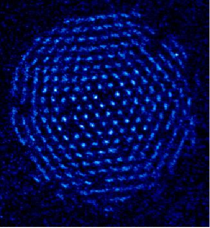
To confine ions a Penning trap uses a combination of a static, cylindrically symmetric electric quadrupole field, and a static magnetic field oriented parallel to the axis of symmetry of the electric field [14]. The electric field provides harmonic axial confinement and the magnetic field confinement in the radial plane in which a single isolated ion will undergo complicated epitrochoid motion. A cloud of ions in the trap will rotate rigidly around the symmetry axis, and the geometry of the cloud depends sensitively on the rotation frequency, varying from cigar-shaped to pancake-shaped. When sufficiently cold, and at the appropriate rotation frequency the ions will crystalize into a disc consisting of a single ion layer. Such a disc is pictured in Fig. 7.

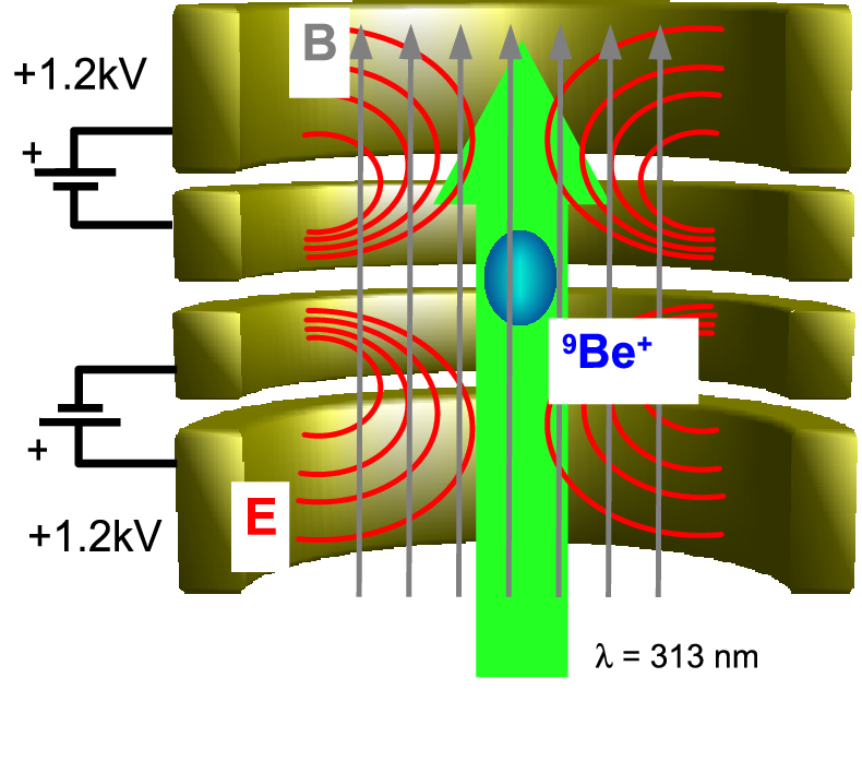
The physical trap, Figure 8, consists of two pairs of stacked cylindrical electrodes onto which static voltages of 1.2 kV are applied to provide the quadrupole electric field. A magnetic field of 4.5 T is provided by a superconducting magnet. Cooling laser beams enter the trap both axially and perpendicular to the trap axis. The ions can be imaged both by a side-view or top-view camera. Taking stroboscopic images with the top-view camera reveals the crystalline structure of the ions, see Fig. 7. For a single plane the ions for a triangular lattice.

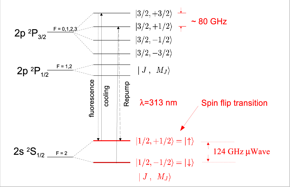
The NIST experiment traps ⁹Be⁺ ions for which the level structure is given in figure 9. The states $|J=1/2,M_{J}=1/2\rangle$ and $|J=1/2,M_{J}=-1/2\rangle$ in the ²S_1/2 hyperfine groundstate manifold serve as the spin states $|\!\uparrow\rangle,|\!\downarrow\rangle$ respectively. They are separated by 124 GHz and controlled by microwaves generated by a p-i-n diode oscillator and injected into the trap through a microwave horn. The microwave field allows high fidelity rotations on the Bloch-sphere. Doppler cooling is achieved by off-resonant scattering of 313 nm light between the states $|\!\uparrow\rangle$ and $|J=3/2,M_{J}=3/2\rangle$ in the ²P_3/2 manifold.

Several technical challenges must be met to successfully implement squeezing as described in the preceding sections.

Recently it was shown that the decoherence effect due to Rayleigh scattering must calculated more carefully [16]. In particular, the Rayleigh decoherence of a spin-superposition depends on the square of the difference between the sum of amplitudes for all scattering processes from the state $|\!\downarrow\rangle$ and the sum of amplitudes for all scattering processes from the state $|\!\uparrow\rangle$. Since the scattering amplitudes depend on the detunings of the light fields, it is possible that for certain choices of detunings the decoherence contributions due to scattering from $|\!\downarrow\rangle$ might add constructively to the contribution from scattering from $|\!\uparrow\rangle$. In fact, even though the drive fields might be far off-resonance, the Rayleigh contribution might be dominant over decoherence due to Raman scattering. The laser detunings used in the Penning trap experiment fall in this regime.

Modern trends in metrology experiments indicate that measurement devices of the future will exploit pure quantum effects to break old barriers in sensitivity. Spin-squeezing is a promising quantum technique for surpassing shot-noise limited measurements. It is a technology currently being pursued by several laboratories world wide with promising progress. This proceedings discussed aspects of spin-squeezing using beryllium ions in a Penning ion trap which will complement recent successes in neutral atom traps.

The Penning trap work is supported by the DARPA OLE program. NIST is an agency of the US government. This work is not subject to US copyright.

We wish to construct properly normalized states generated by$(J_{-})^{q}|\uparrow\uparrow\uparrow...\uparrow\uparrow\rangle$. So

	$\displaystyle(J_{-})^{q}|\uparrow\uparrow\uparrow...\uparrow\uparrow\rangle$	$\displaystyle=$	$\displaystyle(\sum_{j}\hat{\sigma}^{-}_{j})^{q}|\uparrow\uparrow\uparrow...\uparrow\uparrow\rangle$		(21)
		$\displaystyle=$	$\displaystyle\sum_{j_{1},j_{2},...j_{q}}\hat{\sigma}^{-}_{j_{1}}\hat{\sigma}^{-}_{j_{2}}...\hat{\sigma}^{-}_{j_{q}}|\uparrow\uparrow\uparrow...\uparrow\uparrow\rangle.$		(22)

Each index $j_{k}$ in (22) runs from 1 to $N$. However, whenever any two or more operators $\hat{\sigma}^{-}_{j_{k}}$ have the same index, the term will vanish after operation on the state $|\uparrow\uparrow\uparrow...\uparrow\uparrow\rangle$, since a lowering operation cannot be applied to the same particle twice. We therefore need only keep terms in the sum for which every index is different, and of which there are $N(N-1)(N-2)...(N-(q-1))$, so

$$(J_{-})^{q}|\uparrow\uparrow\uparrow...\uparrow\uparrow\rangle=\sum\limits_{j_{1}\neq j_{2}\neq...\neq j_{q}}\hat{\sigma}^{-}_{j_{1}}\hat{\sigma}^{-}_{j_{2}}...\hat{\sigma}^{-}_{j_{q}}|\uparrow\uparrow\uparrow...\uparrow\uparrow\rangle.$$

(23)

Now, after applying all operators $\hat{\sigma}^{-}_{j_{q}}$ there are $q!$ duplicates of each state
$|\uparrow\uparrow\downarrow_{j_{1}}...\downarrow_{j_{2}}...\downarrow_{j_{q}}\uparrow\rangle$. For example, if $q=3$ each of the $3!$ permutations: $\hat{\sigma}^{-}_{1}\hat{\sigma}^{-}_{2}\hat{\sigma}^{-}_{3}$, $\hat{\sigma}^{-}_{1}\hat{\sigma}^{-}_{3}\hat{\sigma}^{-}_{2}$, $\hat{\sigma}^{-}_{2}\hat{\sigma}^{-}_{1}\hat{\sigma}^{-}_{3}$, etc. leads to the same state $|\downarrow\downarrow\downarrow\uparrow...\uparrow\rangle$. So keeping only unique terms we can rewrite (23) as

$$(J_{-})^{q}|\uparrow\uparrow\uparrow...\uparrow\uparrow\rangle=q!\sum\limits_{j_{1}<j_{2}<...<j_{q}}\hat{\sigma}^{-}_{j_{1}}\hat{\sigma}^{-}_{j_{2}}...\hat{\sigma}^{-}_{j_{q}}|\uparrow\uparrow\uparrow...\uparrow\uparrow\rangle.$$

(24)

Notice in (24) the change in indexing of the sum as compared to (23) and the extra factor $q!$. Equation (24) contains $\mathcal{N}=N(N-1)(N-2)...(N-(q-1))/q!$ terms so to normalize it we must divide by $q!\sqrt{\mathcal{N}}=\sqrt{q!N(N-1)(N-2)...(N-(q-1))}$. Finally then, our properly normalized states are

	$\displaystyle\hskip-28.45274pt|\frac{N}{2},\frac{N}{2}-q\rangle\!\!\!\!\!\!$	$\displaystyle=$	$\displaystyle\!\!\!\!\!\!\frac{1}{\sqrt{q!N(N-1)...(N-(q-1))}}(J_{-})^{q}|\uparrow\uparrow\uparrow...\uparrow\uparrow\rangle$		(25)
		$\displaystyle=$	$\displaystyle\!\!\!\!\!\!\frac{\sqrt{q!}}{\sqrt{N(N-1)...(N-(q-1))}}\sum\limits_{j_{<}j_{2}<...<j_{q}}\hat{\sigma}^{-}_{j_{1}}\hat{\sigma}^{-}_{j_{2}}...\hat{\sigma}^{-}_{j_{q}}|\uparrow\uparrow\uparrow...\uparrow\uparrow\rangle.$		(26)

We leave it to the reader to verify that these states will obey the expected raising and lowering relations of angular momentum states:

$$J_{\pm}|J,M_{J}\rangle=\sqrt{J(J+1)-M_{J}(M_{J}\pm 1)}|J,M_{J}\pm 1\rangle.$$

(27)

References

- [1] C. Chou, D. Hume, J. Koelemeij, D. Wineland, and T. Rosenband, Phys. Rev. Lett. 7, 070802 (2010).
- [2] J. Combes and H. Wiseman, J. Opt. B: Quantum Semiclass. 7, 14 (2005).
- [3] J. Appel, P. Windpassinger, D. Oblak, U. Hoff, N. Kjaergaard, and E. Polzik, PNAS 106, 10960 (2009).
- [4] T. Takano, M. Fuyama, R. Namiki, and Y. Takahashi, Phys. Rev. Lett. 102, 033601 (2009).
- [5] M. Riedel, P. Bohi, Y. Li, T. Hansch, A. Sinatra, and P. Treutlein, Nature 464, 1170 (2010).
- [6] C. Gross, T. Zibold, E. Nicklas, J. Esteve, and M. Oberthaler, Nature 464, 1165 (2010).
- [7] I. Leroux, M. Schleier-Smith, and V. Vuletic, Phys. Rev. Lett. 104, 073602 (2010).
- [8] Z. Chen, J. Bohnet, S. Sankar, and J. Thompson, Phys. Rev. Lett. 106, 133601 (2011).
- [9] M. Kitagawa and M. Ueda, Phys. Rev. A 47, 5138 (1993).
- [10] V. Meyer, M. Rowe, D. Kielpinski, C. Sackett, W. Itano, C. Monroe, and D. Wineland, Phys. Rev. Let. 86, 5870 (2001).
- [11] R. Dicke, Phys. Rev. 93, 99 (1954).
- [12] D. Leibfried, B. DeMarco, V. Meyer, D. Lucas, M. Barret, J. Britton, W. Itano, B. Jelenkovic, C. Langer, T. Rosenband, et al., Nature 422, 412 (2003).
- [13] T. Mitchell, J. Bollinger, D. Dubin, X. Huang, W. Itano, and R. Baughman, Science 282, 1290 (1998).
- [14] M. Biercuk, H. Uys, A. Van Devender, N. Shiga, W. Itano, and J. Bollinger, Quant. Inf. Comp. 9, 0920 (2009).
- [15] R. Ozeri, W. Itano, R. Blakestad, J. Britton, J. Chiaverini, J. Jost, C. Langer, D. Leibfried, R. Reichle, S. Seidelin, et al., Phys. Rev. A 75, 042329 (2007).
- [16] H. Uys, M. Biercuk, A. VanDevender, C. Ospelkaus, D. Meiser, R. Ozeri, and J. Bollinger, Phys. Rev. Lett. 105, 200401 (2010).