DESY 11-218
The Higgs boson resonance width from a chiral Higgs-Yukawa model on the lattice
Abstract
The Higgs boson is a central part of the electroweak theory and is crucial to generate masses for quarks, leptons and the weak gauge bosons. We use a 4-dimensional Euclidean lattice formulation of the Higgs-Yukawa sector of the electroweak model to compute physical quantities in the path integral approach which is evaluated by means of Monte Carlo simulations thus allowing for fully non perturbative calculations. The chiral symmetry of the model is incorporated by using the Neuberger overlap Dirac operator. The here considered Higgs-Yukawa model does not involve the weak gauge bosons and furthermore, only a degenerate doublet of top- and bottom quarks are incorporated. The goal of this work is to study the resonance properties of the Higgs boson and its sensitivity to the strength of the quartic self coupling.
Keywords:
Higgs-Yukawa model, Higgs boson resonance, finite size method1 Introduction
The model under consideration is the pure Higgs-Yukawa sector of the electroweak standard model formulated on a 4-dimensional Euclidean space-time lattice. The field content of the model consists of a complex scalar Higgs doublet and a fermion doublet coupled in a chirally invariant way to the scalar sector. Our lattice model closely resembles the weak interaction of the continuum standard model in the limit where the gauge fields are switched off. The chiral nature of the weak interaction is realized in our lattice setup with the help of the Neuberger overlap Dirac operator [1] which allows to incorporate an exact chiral symmetry on the lattice [2].
Within the past years renewed efforts have been undertaken to investigate the lower and upper Higgs boson mass bounds within this model in the framework of lattice field theory [3, 4, 5], see these references also for accounts of earlier lattice investigations of Higgs boson mass bounds. However, the decay width of the Higgs boson was not taken into account in refs. [3, 4] assuming that its effect on the Higgs boson mass is small. The first main aim of this work is to treat the Higgs boson as a true resonance and to investigate the unstable nature of the Higgs boson from first principles. In this way, the assumption of the preceding work [3, 4] can be tested and it can be investigated, whether the Higgs boson mass bounds are affected. The second goal is to determine the Higgs boson width as a function of the quartic self-interaction of the Higgs fields, including large values of the coupling. In particular, we want to investigate, whether in the decay channel of the Higgs boson into massive vector bosons the Higgs boson becomes a broad resonance at large couplings, or whether the width is still rather narrow.
The strategy to determine the Higgs boson resonance parameters is the analysis of the scattering phases. The computation of the scattering phase within lattice field theory is in turn based on the determination of the volume dependence of energy eigenvalues [6]. An extension of the finite size method of ref. [6], which was formulated in the center of mass frame, has been proposed in [7] and is based on the analysis of the energy levels within a moving frame. The method is complementary to the original method and allows to obtain more energy levels on the same underlying field configurations. We employ this method here to reduce the errors on our extraction of the scattering width and the resonance mass, which we are then able to determine at the level.
2 The model
The Higgs-Yukawa model is defined by the Lagrangian and the corresponding generating functional for the Green functions of the theory. With regard to the lattice formulation of the model, the Euclidean version of the model will be considered here. The particle content contains the scalar sector and the heaviest quark doublet consisting of the top and the bottom quark. Due to the neglection of gauge bosons the Lagrangian exhibits a global inner symmetry rather than a local (gauge) symmetry. The Euclidean action is given by
| (1) |
Here, , and denote the bare scaler mass, the bare quartic coupling and the bare top (bottom) Yukawa coupling, respectively. It is common in lattice field theory to rewrite the scalar sector by rescaling the fields with a factor and furthermore, the scalar doublet can be expressed as a quarternion
| (2) |
The rescaled fields are:
The scalar fields in the usual notation of eq. (1) can be recovered by identifying
where are the original, complex valued scalar fields.
In 1982 Ginsparg and Wilson [8] proposed a relation which defines a class of lattice Dirac operators and which is since then known as the Ginsparg-Wilson relation
| (3) |
Here is the lattice spacing and is a positive constant. The Ginsparg-Wilson relation can be utilized to construct a lattice modified chiral symmetry which recovers the desired continuum chiral symmetry in the limit [2]. The modified lattice projectors for the left and right handed components are given by
The modified projectors are used to define the chiral components of the spinor fields on the lattice
As in the continuum theory the free part of the fermion Lagrangian can be written as a sum of the left and right handed lattice spinor fields
The modified projectors allow to formulate a theory of continuum-like left- and right handed fermions on the lattice for any non-vanishing value of the lattice spacing .
In order to specify the lattice action, a Ginsparg-Wilson type Dirac operator has to be introduced. The here presented results are based on the Neuberger overlap operator [1], which satisfies the Ginsparg-Wilson relation and is given by
| (4) |
is chosen to be in this work and denotes the Wilson Dirac operator. In [9] it has been demonstrated that the Neuberger overlap operator is, despite its complicated form, a local operator.
The full Euclidean discretized action is given by
| (5) |
In the following, the lattice spacing is set to unity. It can be given a physical value by identifying the vacuum expection value on the lattice, with the measured value of GeV. As mentioned before, the couplings are scaled by the parameter. The parameterization of the Lagrangian in (1) can by recovered with the identities:
The here considered Higgs-Yukawa model has already been studied extensively. In refs. [10, 11] the phase structure has been determined, lower and upper Higgs boson mass bounds have been obtained in [3, 4] and also an extension to a possible fourth quark generation has been discussed in [12]. Many details of the model, its numerical implementation and algortihmic aspects can be found in ref. [13].
3 Resonances from lattice simulations
The method to compute the resonance parameters in finite volume was proposed in [6]. It has been successfully employed for the case of the Higgs boson mass in the pure theory [14]; here we want to extend the method to the Higgs-Yukawa model as considered in this work.
Let us start with the optical theorem which states that the total cross section in the elastic region of forward scattering is given by
| (6) |
denotes the centre of mass momentum and is the centre of mass energy of the two incomming particles with four momentum and , . is the spherical decomposition of the interacting part of the S-Matrix
The total cross section exhibits a peak near a resonance which can be well parameterized with a Breit-Wigner function containing the resonance mass and the width ,
| (7) |
where we have also expressed the total cross section in eq. (6) in terms of the scattering phases .
In order to develop a general method to extract the scattering phase from the energy levels in a finite box, it is sufficient to investigate the problem in non-relativistic quantum mechanics. The non-relativistic result can then be transferred to the case of quantum field theory. This remarkable result has been demonstrated in refs. [15, 16].
As a result of these works the computation of the scattering phase in which we are interested in, proceeds as follows. The first step is to compute the energies of the two-particle massive Goldstone system, , from which the value of can be extracted. Knowing , the scattering phase is obtained from
The analysis of scattering phases has been extended to moving frames in [7, 17, 18], where one of the two particles is at rest. The method is complementary to the centre of mass frame and allows to compute more data for the scattering phases from the same configurations. The obtained two particle energies have to be translated back to the centre of mass frame. In general, the choice of a moving frame implies that one has to consider irreducible representations of a subgroup of the cubic group. The remaining symmetry depends on the selected directions of the moving frame. The here used irreducible representations are given in [7]. The modification of the relation between the two particle energy in the moving frame and the scattering phase is given by
where denotes the momentum which has been transferred back to the centre of mass frame by a Lorentz boost. The modified Zeta function is defined by
The vector is related to the total momentum of the moving frame . is the usual Lorentz factor. Below are some definitions which are needed to compute the modified Zeta function
denotes the two particle energy in the moving frame which can be computed with time slice correlators. The corresponding observables are defined in the next section. and is a decomposition of the vector in its parallel and perpendicular parts with respect to the centre of mass velocity
4 Numerical results
The Higgs boson decays dominantly to any even number of Goldstone bosons, if kinematically allowed. The physical set-up chosen here allows always for such a decay, i.e. we were always working in the elastic scattering region. In order to achieve this situation, external currents were introduced, providing appropriate masses to the else mass-less Goldstone bosons. The bare parameters used in our simulations are given in table 4. The corresponding physical value of the cut-off, the Higgs boson propagator mass, the Goldstone boson mass and the obtained top quark mass are summarized in table 4.
The table summarizes the bare parameters for the Monte Carlo simulations which were performed in order to determine the scattering phases. denotes an external current which is coupled to one component of the scalar field. is adjusted such that the the ratio of the Higgs boson mass and and the Goldstone boson mass is approximately (see table 4), which ensures that the Higgs boson decays into any even number of Goldstone bosons.
The table summarizes the obtained masses in lattice units for the bare parameters given in table 4. The Higgs and Goldstone boson masses, and respectively, are extracted from the propagator neglecting the width. The quark mass is computed from the corresponding time slice correlator and the last columns show the renormalized vacuum expectation value and the cut-off (). For the smaller lattices we have typically used 20000 and for the largest lattice typically 10000 configurations. The autocorrelation times were about one in all cases, see also [13]. Note that, due to a technical problem, for the determination of at we have used a significantly smaller statistics than at the other simulation points. [GeV] [GeV]
The Goldstone theorem ensures that the Goldstone bosons are massless. Due to an external current which couples to one of the components of the scalar fields in the complex doublet, the symmetry is broken explicitly in the Lagrangian. The Goldstone bosons acquire a mass and they form a vector under cubic rotations. The magnitude of the current is chosen such that the ratio of the Higgs boson mass to the Goldstone boson mass is roughly . Here and below the superscript in and denotes that the mass was extracted from the analysis of the momentum space propagator. This numerically computed propagator was then fitted to a formula motivated from perturbation theory and the real part of the complex pole of this fit function has been identified with the Higgs boson mass, see refs. [3, 4, 12, 13].
The Higgs field is a singlet under cubic rotations and transforms as elements in the representation. The two particle energies discussed in the previous section are constructed from the two particle Goldstone singlet as it has the same quantum numbers as the Higgs boson.
The analysis of the resonance parameters involves several lattice volumes with identical bare parameters in order to compute the momentum dependence of the scattering phase. As shown in table 4, there are three distinct set of simulation parameters which shall be characterized with the value of the bare quartic coupling (). For each of the three values of the quartic coupling the simulations were performed on lattice volumes up to . In the following the two particle energies of the two Goldstone boson states will be discussed. Once these energy levels are known, the unstable nature of the Higgs boson can be studied by the method described in the preceeding chapter.
The Goldstone bosons are stable particles such that their ground state energy can be calculated from the two point time correlation function. The concept of time correlators is widely used in lattice field theory and there are reliable techniques to extract mass eigenvalues from such correlators. The method of choice in this work, is the analysis of the correlation matrix [15, 19]. The correlation matrix built from an operator is given by
where is the temporal size of the lattice. Throughout this chapter the temporal extent will be . The subscript denotes that the disconnected part of the correlator has been subtracted. It has been shown in [15] that the eigenvalues of the correlation matrix decay exponentially with rising time separation . In the following the operators which contribute to the two Goldstone system are collected.
The definition of the observables in the centre of mass frame is given by
The correlation matrix is thus a matrix. and denote the standard, zero momentum projected Higgs and Goldstone boson interpolating fields , , see e.g. [14, 13].
In order to collect more data for the scattering phases, the modification of the method to a moving frame was analysed as well. The moving frame is characterised by a constant vector which indicates the momentum of the frame. The observables for the moving frame are constructed such that one of the Goldstone bosons is at rest while the other can take any momentum allowed on the lattice. The selection of a constant vector breaks the cubic symmetry and thus special care is needed while constructing the observables. Fortunately, it turns out that the sector does not need much modification and explicit relations are given in [7]. The lowest energy eigenstates are associated to the lowest possible relative momentum and thus only moving frames with momentum and permutations thereof will be considered. The observables are ( is the unit three-vector in direction )
The correlation matrix in the moving frame is then given by
The energy levels obtained from the moving frame are connected to energy levels in the corresponding centre of mass frame by Lorentz transformation.
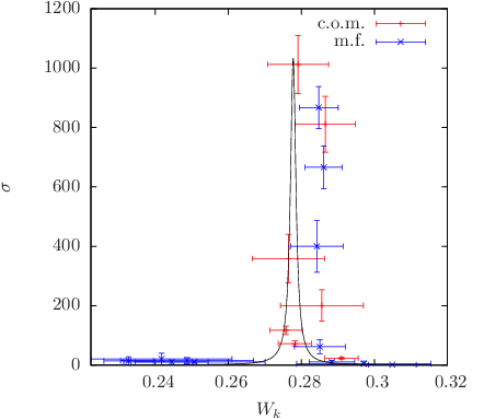
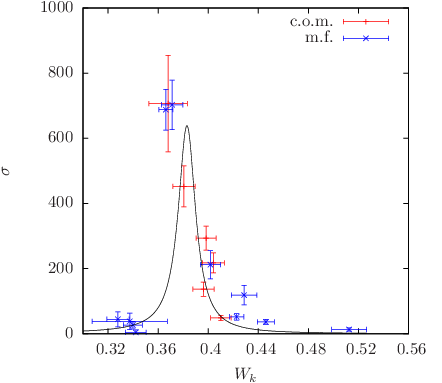
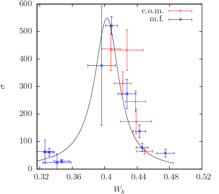
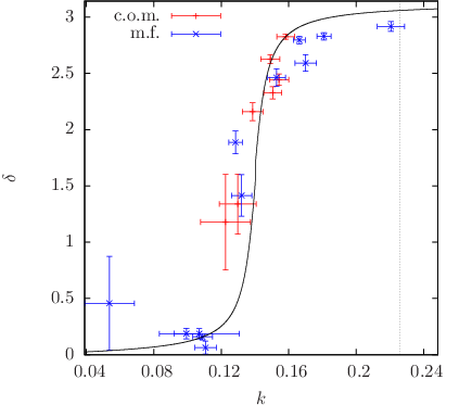
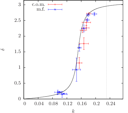
Fig. 1 shows the obtained cross sections and Fig. 2 the obtained scattering phases for the three different physical situations (different values of ) we have used. The cross sections are plotted against the energy while the scattering phase, which take values in the interval , are plotted against the momentum . If the scattering phase passes through it indicates the existence of a resonance. Hence, all three setups involve an unstable Higgs boson. The cross section can be decomposed into spherical harmonics and is parametrised by the scattering phase
| (8) |
which becomes
when the contribution of the higher angular momenta are neglected. We use a fit function to describe our data for which is motivated by a Breit-Wigner form and allows us to determine the resonance mass and the width :
| (9) |
In fig. 1, the solid curve shows the result of the fit for the cross section and in fig. 2 we show the corresponding scattering phases. The scattering phase is directly related to the cross section in equation (9) as can be seen in equation (7). Given the scattering phases, the cross section can be obtained from equation (8) setting .
 |
 |
 |
| (a) | (b) | (c) |
 |
 |
 |
| (a) | (b) | (c) |
Finally table 4 summarizes the results for the Higgs boson mass obtained by different approaches. The physical (resonance) Higgs boson mass is compared to the mass obtained from the Higgs boson propagator and the energy eigenvalue from the correlation matrix analysis (GEVP) which corresponds to the Higgs boson mass. The results for and the GEVP were obtained after an extrapolation to infinite volume, see fig. 3 for the example of the infinite volume extrapolation of the eigenvalue from the GEVP. For completeness, we also show the finite size behaviour of the renormalized vacuum expectation value and the top quark mass in fig. 4.
The table summarizes the obtained final results on the resonance mass and the resonance width of the Higgs boson. denotes the bare quartic coupling. is the cut-off of the theory. The following two columns display the resonance parameters computed from the scattering phases. The per degree of freedom from the fits to obtain the resonance parameters are , and for , and , respectively. is the width obtained from perturbation theory where a non vanishing mass for the Goldstone bosons has been considered [20]. Finally the mass extracted from the propagator as well as the eigenvalue corresponding to the Higgs boson mass computed with the help of the correlation matrix is shown. [GEV] GEVP
 |
 |
 |
| (a) | (b) |
The simulations at and belong to a cut-off of around TeV. It was necessary to reduce the cut off to GeV for the smallest quartic coupling in order to meet the resonance condition (). As one can see from table 4, the Higgs boson mass is still well below the cut off. Especially for the smallest quartic coupling the resonance region is very small () which in turn necessitates large lattice volumes in order to obtain energy eigenvalues which lead to scattering phases near the resonance mass. The plots in fig. 1 and fig. 2 show that the analysis of the moving frame can help significantly to extract reliable results.
5 Conclusion
In this letter we have investigated the resonance parameters of the standard model Higgs boson from simulations on a Euclidean lattice in the limit of the electroweak theory where the gauge fields are neglected. In this situation the Higgs boson decays into massive vector bosons. The resonance mass and the width of the Higgs boson is computed using the finite size method proposed in [6], applicable for the center of mass frame, combined with the extension to a moving frame as proposed in [7]. Using both kind of Lorentz frames a large number of scattering phases could be obtained which allowed us to compute the Higgs boson resonance mass and width with an accuracy of for the resonance mass and for the width, see table 4.
We have employed three values of the quartic coupling of the Higgs field ranging from small perturbative values to with parameters corresponding to a large renormalized quartic coupling. In all three cases the Higgs boson width is not larger than about with respect to the resonance mass. Therefore, the corresponding total cross section exhibits a clear resonance peak even at the strongest value of the quartic coupling.
The values of the resonance mass we have extracted here are in very good agreement with earlier determinations [3, 4] where the Higgs boson width has been neglected. This finding provides confidence to and justifies a posteriori the Higgs boson mass bounds determined in [3, 4]. In addition, a comparison of the Higgs boson width with results from perturbation theory reveals a very good agreement as can be seen in table 4.
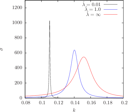
Figure 5 summarizes the obtained total cross sections for the three different values of the bare quartic couplings. The displayed curves correspond to the fits shown in figure 1 using the parameterization of eq. (9). It will be interesting to apply the techniques used in this paper for the investigation of the Higgs boson mass width in presence of a possible fourth fermion generation, where non-perturbative effects might appear for very heavy masses of the fourth generation quarks. Simulations in this direction have been started already [12].
Acknowledgments
We gratefully acknowledge the support of the DFG through the DFG-project Mu932/4-2. The numerical computations have been performed on the HP XC4000 System at the Scientific Supercomputing Center Karlsruhe and on the SGI system HLRN-II at the HLRN Supercomputing Service Berlin-Hannover.
References
- [1] H. Neuberger, Phys. Lett. B427 (1998) 353–355.
- [2] Lüscher, M., Phys. Lett. B428 (1998) 342–345.
- [3] P. Gerhold, K. Jansen, JHEP 04 (2010) 094.
- [4] P. Gerhold, K. Jansen, JHEP 07 (2009) 025.
- [5] Z. Fodor, K. Holland, J. Kuti, D. Nogradi, C. Schroeder, PoS LAT2007 (2007) 056.
- [6] Lüscher, M., Nucl. Phys. B354 (1991) 531–578.
- [7] K. Rummukainen, S. A. Gottlieb, Nucl. Phys. B450 (1995) 397–436.
- [8] P. H. Ginsparg, K. G. Wilson, Phys. Rev. D25 (1982) 2649.
- [9] Hernandez, P. and Jansen, K. and Lüscher, M., Nucl. Phys. B552 (1999) 363–378.
- [10] P. Gerhold, K. Jansen, JHEP 10 (2007a) 001.
- [11] P. Gerhold, K. Jansen, JHEP 09 (2007b) 041.
- [12] P. Gerhold, K. Jansen, J. Kallarackal, JHEP 01 (2011) 143.
- [13] P. Gerhold, Ph.D. Thesis (2010).
- [14] Göckeler, M. and Kastrup, H. A. and Westphalen, J. and Zimmermann, F., Nucl. Phys. B425 (1994) 413–448.
- [15] Lüscher, M. and Wolff, U., Nucl. Phys. B339 (1990) 222–252.
- [16] Lüscher, M., Commun. Math. Phys. 105 (1986) 153–188.
- [17] X. Feng, K. Jansen, D. B. Renner, Phys.Rev. D83 (2011) 094505.
- [18] X. Feng, K. Jansen, D. B. Renner, PoS LAT2010 (2010) 104.
- [19] B. Blossier, M. Della Morte, G. von Hippel, T. Mendes, R. Sommer, JHEP 04 (2009) 094.
- [20] Lüscher, M. and Weisz, P., Nucl. Phys. B318 (1989) 705.