Higher order duality and toric embeddingsThanks: AD is partially supported by UBACYT 20020100100242, CONICET PIP 112-200801-00483, and ANPCyT PICT 2008-0902, Argentina. SDR is partially supported by VR grant NT:2010-5563

Alicia Dickenstein Address: Alicia Dickenstein
Department of Mathematics, FCEN
Universidad de Buenos Aires
and IMAS - CONICET
Ciudad Universitaria - Pab. I
C1428EGA Buenos Aires
Argentina Email address: alidick@dm.uba.ar URL: mate.dm.uba.ar/˜alidick , Sandra Di Rocco Address: Sandra Di Rocco
Department of Mathematics
Royal Institute of Technology (KTH)
10044 Stockholm
Sweden Email address: dirocco@math.kth.se URL: www.math.kth.se/˜dirocco and Ragni Piene Address: Ragni Piene
CMA/Department of Mathematics
University of Oslo
P.O.Box 1053 Blindern
NO-0316 Oslo
Norway Email address: ragnip@math.uio.no URL: www.mn.uio.no/math/english/people/aca/ragnip/index.html

Abstract.

The notion of higher order dual varieties of a projective variety, introduced by Piene in 1983, is a natural generalization of the classical notion of projective duality. In this paper we study higher order dual varieties of projective toric embeddings. We express the degree of the second dual variety of a $2$ -jet spanned embedding of a smooth toric threefold in geometric and combinatorial terms, and we classify those whose second dual variety has dimension less than expected. We also describe the tropicalization of all higher order dual varieties of an equivariantly embedded (not necessarily normal) toric variety.

Dedicated to the memory of our friend Mikael Passare (1959–2011)

Key words and phrases:

toric variety, higher order projective duality, tropicalization

2010 Mathematics Subject Classification

14M25,14T05

1. Introduction

Projective duality of algebraic varieties is a classical subject in algebraic geometry. Given an embedding $X\hookrightarrow\mathbb{P}^{m}$ (over an algebraically closed field of characteristic $0$ ), the Zariski closure of the set of hyperplanes $H\in{\mathbb{P}^{m}}^{\vee}$ tangent to $X$ at a smooth point is an irreducible variety called the dual variety and denoted by $X^{\vee}$ . There is a natural generalization of projective duality, introduced in [24]. One defines the $k$ -th dual variety $X^{(k)}\subset{\mathbb{P}^{m}}^{\vee}$ of $X\subset\mathbb{P}^{m}$ as the Zariski closure of the set of hyperplanes tangent to $X$ to the order $k$ at some smooth point $x\in X$ (see Definition 2.1.)

The purpose of this paper is to introduce higher order dual varieties for toric embeddings and give different characterizations. Projective duality for toric varieties is of particular interest because of the connection with convex geometry and combinatorics.

Consider a (non-degenerate) embedding of a projective variety $X\hookrightarrow\mathbb{P}^{m}$ . For $k=1$ , the expected codimension of the dual variety $X^{\vee}=X^{(1)}$ is $1$ . When this is not the case, $X$ is said to be (dual) defective. Defective embeddings have been studied and classified (see e.g. [10, 11] and, for the toric case, [28, 4]). A combinatorial characterization of the dimension, as well as a positive formula (that is, a formula involving only positive terms) for the degree of the dual variety of toric embeddings via tropical geometry, were recently given in [8].

Likewise, for any $k$ , the expected dimension of $X^{(k)}$ equals $m+n-\ell$ , where $n=\dim(X)$ and $\ell$ is the generic rank of the $k$ -jet map (see Definition 2.2). Then $X$ is said to be $k$ -defective when $X^{(k)}$ has lower dimension than expected. Typical examples of varieties that are $k$ -defective for $k\geq 2$ are scrolls. Higher order dual varieties of scrolls over curves have been studied in [23] and [20]. Notice that in this case the osculating spaces do not have maximal dimension (see Example 2.3.) We shall mainly restrict our attention to $k$ -jet spanned embeddings, i.e., embeddings with the property that the $k$ -jet map has maximal rank $\ell=\binom{n+k}{n}$ at every smooth point. However, in Section 4 we shall examine the case of rational normal scrolls, which are typical examples of embeddings that are not $k$ -jet spanned.

Smooth $k$ -jet spanned embeddings of surfaces which are $k$ -defective have been classified in [19]. In fact, there is only one defective case, namely $(\mathbb{P}^{2},{\mathcal{O}}(k)).$ This result generalizes the classification of dual defective smooth surfaces. In Corollary 3.10 we extend this classification to smooth toric threefolds for $k=2$ . Furthermore, we give in Theorem 3.7 a formula for the degree of the second dual variety in terms of combinatorially defined quantities (see also Corollary 3.9). We summarize these results in the following statement.

Let $(X,\mathcal{L})$ be a $2$ -jet spanned toric embedding of a smooth threefold, corresponding to a $2$ -regular lattice polytope $P$ of dimension three (cf. Definition 3.2 and Proposition 3.3 for the notion of $2$ -regularity). Then $X$ is $2$ -defective if and only if $(X,\mathcal{L})=(\mathbb{P}^{3},\mathcal{O}(2))$ , in which case the second dual variety $X^{(2)}$ is empty. Moreover:

1)

$\deg X^{(2)}=120$ if $(X,\mathcal{L})=(\mathbb{P}^{3},\mathcal{O}(3))$ .
2)

$\deg X^{(2)}=6(8(a+b+c)-7)$ if $(X,\mathcal{L})=(\mathbb{P}(\mathcal{O}_{\mathbb{P}^{1}}(a),\mathcal{O}_{\mathbb{P}^{1}}(b),\mathcal{O}_{\mathbb{P}^{1}}(c)),2\xi)$ , where $a,b,c\geq 1$ and $\xi$ denotes the tautological line bundle.

In all other cases,

\deg_{2}\,X^{(2)}=62\operatorname{Vol}(P)-57\mathcal{F}+28\mathcal{E}-8\mathcal{V}+58\operatorname{Vol}(P^{\circ})+51\mathcal{F}_{1}+20\mathcal{E}_{1}

where $\operatorname{Vol}(P)$ , $\mathcal{F}$ , $\mathcal{E}$ (resp. $\operatorname{Vol}(P^{\circ})$ , $\mathcal{F}_{1}$ , $\mathcal{E}_{1}$ ) denote the (lattice) volume, area of facets, length of edges of $P$ (resp. of the convex hull of the interior lattice points of $P$ ), and $\mathcal{V}$ is the number of vertices of $P$ . (The definition of $\deg_{2}\,X^{(2)}$ is given in (3), cf. also Proposition 2.5.)

A (not necessarily normal) non-degenerate equivariantly embedded projective toric variety is rationally parameterized by monomials with exponents a lattice point configuration $\mathcal{A}=\{r_{0},\dots,r_{m}\}\subset\mathbb{Z}^{n}$ (see [14]). That is, $\mathcal{A}$ is a subset of the lattice points in the lattice polytope $P=\operatorname{Conv}(\mathcal{A})$ . We denote this variety by $X_{\mathcal{A}}$ . In Section 5 we give the description of the tropicalization $\operatorname{trop}(X_{\mathcal{A}}^{(k)})$ of the $k$ -th dual variety of $X_{\mathcal{A}}$ for any $k$ . By a result of Bieri and Groves [3], $\operatorname{trop}(X_{\mathcal{A}}^{(k)})$ is a rational polyhedral fan of the same dimension as

X_{\mathcal{A}}^{(k)}\cap\{x\in{\mathbb{P}^{m}}^{\vee},\,x_{i}\not=0\text{ for all }i=0,\dots,m\}.

In Theorems 5.3 and 5.6 we present characterizations of $\operatorname{trop}(X_{\mathcal{A}}^{(k)})$ , which are direct generalizations of the corresponding results for the classical dual variety obtained in [8, 9]. This leads to a combinatorial characterization of the dimension and to a positive formula for the degree of higher dual varieties (cf. Remark 5.5).

2. Higher order dual varieties

Let $\iota\colon X\hookrightarrow\mathbb{P}^{m}$ be an embedding of a complex non-degenerate algebraic variety of dimension $n$ . The $k$ -th dual variety $X^{(k)}\subset{\mathbb{P}^{m}}^{\vee}$ of $\iota$ is the Zariski closure of the set of hyperplanes tangent to $X$ to the order $k$ at some smooth point $x\in X$ . Let us make the concept of tangency to a certain order more precise. Recall that a hyperplane $H$ is tangent to $X$ at a smooth point $x$ if and only if $H$ contains the embedded tangent space $\mathbb{T}_{X,x}$ . Let $(x_{1},...,x_{n})$ be a local system of coordinates around $x$ , so that the maximal ideal is ${\mathfrak{m}}_{x}=(x_{1},...,x_{n})$ in ${\mathcal{O}}_{X,x}$ , and let $\mathcal{L}:=\iota^{*}({\mathcal{O}}_{\mathbb{P}^{m}}(1)).$

The vector space $\mathcal{L}/{\mathfrak{m}}_{x}^{k+1}\mathcal{L}$ is the fibre at $x\in X$ of the $k$ -th principal parts (or jet) sheaf ${\mathcal{P}}_{X}^{k}(\mathcal{L})$ , which has generic rank $\binom{n+k}{n}$ . We identify $H^{0}(\mathbb{P}^{m},{\mathcal{O}}(1))\otimes{\mathcal{O}}_{X}\simeq{\mathcal{O}}_{X}^{m+1}$ . The $k$ -th jet map (of coherent sheaves)

j_{k}:{\mathcal{O}}_{X}^{m+1}\to{\mathcal{P}}_{X}^{k}(\mathcal{L})

is given fiberwise by the linear map $j_{k,x}:H^{0}(\mathbb{P}^{m},\mathcal{O}(1))\to H^{0}(X,\mathcal{L})\to H^{0}(X,\mathcal{L}/{\mathfrak{m}}_{x}^{k+1}\mathcal{L})$ , induced by the map of ${\mathcal{O}}_{X}$ -modules $\mathcal{L}\to\mathcal{L}/{\mathfrak{m}}_{x}^{k+1}\mathcal{L}$ . So if $s\in H^{0}(X,\mathcal{L})$ , $j_{k,x}(s)$ is the Taylor series expansion up to order $k$ of $s$ with respect to the local coordinates $x_{1},\ldots,x_{n}$ . With respect to the natural basis $\{1,dx_{1},\ldots,dx_{n},\ldots,dx_{n}^{k}\}$ for ${\mathcal{P}}_{X}^{k}(\mathcal{L})_{x}$ , it can be written as

j_{k,x}(s)=(s(x),\frac{\partial s}{\partial x_{1}}(x),\ldots,\frac{\partial s}{\partial x_{n}}(x),\frac{1}{2}\frac{\partial^{2}s}{\partial x_{1}^{2}}(x),\ldots,\frac{1}{2}\frac{\partial^{2}s}{\partial x_{n}^{2}}(x),\ldots).

Thus, $\mathbb{P}(\operatorname{Im}(j_{1,x}))=\mathbb{P}({\mathcal{P}}_{X}^{1}(\mathcal{L})_{x})={\mathbb{T}}_{X,x}\cong\mathbb{P}^{n}$ is the embedded tangent space at the point $x$ . More generally, the linear space $\mathbb{P}(\operatorname{Im}(j_{k,x}))={\mathbb{T}}^{k}_{X,x}$ is called the $k$ -th osculating space at $x.$

Definition 2.1.

We say that a hyperplane $H$ is tangent to $X$ to order $k$ at a smooth point $x$ if ${\mathbb{T}^{k}_{X,x}}\subseteq H$ . The $k$ -th dual variety is

(1)

X^{(k)}:=\overline{\{H\in{\mathbb{P}^{m}}^{\vee}\;|\,H\supseteq{\mathbb{T}^{k}_{X,x}}\text{ for some }\,x\in X_{\rm sm}\}}.

In particular, $X^{(1)}=X^{\vee}$ . Alternatively, one can define $X^{(k)}$ as the closure of the image of the map

(2)

\gamma_{k}:\mathbb{P}(({\rm Ker}\,j_{k})^{\vee}|_{X_{k{\rm-cst}}})\to{\mathbb{P}^{m}}^{\vee},

where $X_{k{\rm-cst}}$ denotes the open set of $X$ where the rank of $j_{k}$ is constant. Note that $X^{(k)}\subseteq X^{(k-1)}$ . Moreover, $X^{(2)}$ is contained in the singular locus of $X^{\vee}$ , since a necessary condition for a point $H\in X^{\vee}$ to be smooth, is that the intersection $H\cap X$ has a singular point of multiplicity 2: if $H\supseteq{\mathbb{T}^{k}_{X,x}}$ for $k\geq 2$ , then $H\cap X$ has a singular point of multiplicity $\geq k+1$ .

Definition 2.2.

We say that the embedding $\iota\colon X\hookrightarrow\mathbb{P}^{m}$ is $k$ -jet spanned at a smooth point $x\in X$ if the $k$ -th osculating space to $X$ at $x$ has the maximal dimension, $\binom{n+k}{k}-1$ , or, equivalently, the map $j_{k,x}$ is surjective. We say that $\iota$ is $k$ -jet spanned if it is $k$ -jet spanned at all smooth points $x\in X$ .

Example 2.3.

Consider the Segre embedding $\mathbb{P}^{t}\times\mathbb{P}^{s}\hookrightarrow\mathbb{P}^{(t+1)(s+1)-1}$ . Any hyperplane section is given, locally around a smooth point with local coordinates $(x_{1},\ldots x_{t},y_{1},\ldots,y_{s})$ , by the vanishing of a polynomial of the form $c_{0}+\sum_{i=1}^{t}c_{i0}x_{i}+\sum_{j=0}^{s}c_{0j}y_{j}+$ $\sum_{i=1,\ldots t,j=1,\ldots s}c_{ij}x_{i}y_{j}.$ One sees that $\dim{\mathbb{T}^{2}_{X,x}}=(t+1)(s+1)-1<\binom{s+t+2}{2}-1$ . In fact, the $2$ -jets corresponding to $\frac{\partial^{2}}{\partial x_{i}^{2}}$ and $\frac{\partial^{2}}{\partial y_{j}^{2}}$ are not “generated by the embedding.”

If the embedding $\iota$ is (generically) $k$ -jet spanned, the (generic) rank of $j_{k}$ is maximal, namely $\binom{n+k}{k}$ . When $\iota$ is generically $k$ -jet spanned and the map $\gamma_{k}\colon\mathbb{P}({\rm Ker}\,j_{k}^{\vee})\to{\mathbb{P}^{m}}^{\vee}$ is generically finite, the dimension of $X^{(k)}$ is equal to $m+n-\binom{n+k}{k}$ . When the general fibers of $\gamma_{k}$ have positive dimension, the $k$ -dual variety has lower dimension than expected, and in this case we say that the embedding is $k$ -defective, with positive $k$ -dual defect

\operatorname{def}_{k}(X):=m+n-\binom{n+k}{n}-\dim X^{(k)}.

When $X^{(k)}$ has the expected dimension, we set

(3)

\deg_{k}X^{(k)}:=\deg(\gamma_{k})\deg X^{(k)}.

The notion of $k$ -jet spannedness at a point can be generalized in the following way.

Definition 2.4.

An embedding $\iota\colon X\hookrightarrow\mathbb{P}^{m}$ , with $\mathcal{L}=\iota^{*}\mathcal{O}(1)$ , is said to be $k$ -jet ample if for every collection of points $x_{1},\ldots,x_{t}\in X$ and integers $k_{1},\ldots,k_{t}$ such that $\sum k_{i}=k+1$ , the map $H^{0}(\mathbb{P}^{m},\mathcal{O}(1))\to H^{0}(X,\mathcal{L})\to\oplus_{i=1}^{t}H^{0}(X,\mathcal{L}/m_{x_{i}}^{k_{i}}\mathcal{L})$ is surjective.

Note that $1$ -jet ampleness is the same as very ampleness. For more details and characterizations of $k$ -jet ampleness for several classes of embeddings we refer the reader to [27, 1].

The following is essentially proven in Theorem 1.4 and Proposition 2.4 in [18]. We give a proof for completeness, and in order to include (c). As usual, $c_{i}(\mathcal{E})$ denotes the $i$ th Chern class of a vector bundle $\mathcal{E}$ .

Proposition 2.5.

Assume $X$ is a smooth variety of dimension $n$ , and that the embedding $\iota\colon X\hookrightarrow\mathbb{P}^{m}$ is $k$ -jet spanned. Then

(a)

the embedding $\iota$ is $k$ -defective if and only if $c_{n}(\mathcal{P}_{X}^{k}(\mathcal{L}))=0$ ;
(b)

if $\iota$ is not $k$ -defective, then $\deg_{k}X^{(k)}=c_{n}(\mathcal{P}^{k}_{X}(\mathcal{L}))$ ;
(c)

if $\iota$ is generically $(k+1)$ -jet spanned, then the embedding is not $k$ -defective;
(d)

if $\iota$ is $(k+1)$ -jet ample, then $\deg(\gamma_{k})=1$ , and thus $\deg_{k}X^{(k)}=\deg X^{(k)}$ .

Proof.

Let $\mathcal{K}_{k}$ denote the kernel of the $k$ th jet map $j_{k}\colon\mathcal{O}_{X}^{m+1}\to\mathcal{P}_{X}^{k}(\mathcal{L})$ . Because $X$ is smooth, $\mathcal{P}_{X}^{k}(\mathcal{L})$ is a locally free sheaf, with rank $\binom{n+k}{k}$ . Then, since $\iota$ is $k$ -jet spanned and thus $j_{k}$ is surjective, the sheaf $\mathcal{K}_{k}$ is also locally free, with rank $m+1-\binom{n+k}{k}$ . So the sequence

0\to\mathcal{K}_{k}\to\mathcal{O}_{X}^{m+1}\to\mathcal{P}_{X}^{k}(\mathcal{L})\to 0

is exact. Set $\pi\colon\mathbb{P}(\mathcal{K}_{k}^{\vee})\to X$ , and consider the composed map

\gamma_{k}\colon\mathbb{P}(\mathcal{K}_{k}^{\vee})\subset X\times{\mathbb{P}^{m}}^{\vee}\to{\mathbb{P}^{m}}^{\vee}.

Then $X^{(k)}$ is equal to the image of $\gamma_{k}$ and $\mathcal{O}_{\mathbb{P}(\mathcal{K}_{k}^{\vee})}(1)=\gamma_{k}^{*}\mathcal{O}_{{\mathbb{P}^{m}}^{\vee}}(1)$ . From the exact sequence above we have

c(\mathcal{P}^{k}_{X}(\mathcal{L}))=c(\mathcal{K}_{k})^{-1},

and since $c(\mathcal{K}_{k})^{-1}=s(\mathcal{K}_{k}^{\vee})$ , where $s$ denotes the Segre class, we have

c_{n}(\mathcal{P}^{k}_{X}(\mathcal{L}))=s_{n}(\mathcal{K}_{k}^{\vee})=\pi_{*}c_{1}(\mathcal{O}_{\mathbb{P}(\mathcal{K}_{k}^{\vee})}(1))^{n+m-\binom{n+k}{k}},

where the last equality is a well known expression for the $n$ th Segre class.

(a) and (b): Assume $\dim X^{(k)}=m+n-\binom{n+k}{k}-\operatorname{def}_{k}(X),$ with $\operatorname{def}_{k}(X)>0$ . Then, for dimension reasons, $c_{1}(\mathcal{O}_{{\mathbb{P}^{m}}^{\vee}}(1))^{n+m-\binom{n+k}{k}}|_{X^{(k)}}=0$ , therefore $c_{1}(\mathcal{O}_{\mathbb{P}(\mathcal{K}_{k}^{\vee})}(1))^{n+m-\binom{n+k}{k}}=0$ , and hence also $c_{n}(\mathcal{P}^{k}_{X}(\mathcal{L}))=0$ .

Assum instead that $\dim X^{(k)}=m+n-\binom{n+k}{k}$ . Then $\gamma_{k}$ is generically finite, and

\deg\gamma_{k}\cdot\deg X^{(k)}=c_{1}(\mathcal{O}_{\mathbb{P}(\mathcal{K}_{k}^{\vee})}(1))^{n+m-\binom{n+k}{k}}=\pi_{*}c_{1}(\mathcal{O}_{\mathbb{P}(\mathcal{K}_{k}^{\vee})}(1))^{n+m-\binom{n+k}{k}}=c_{n}(\mathcal{P}^{k}_{X}(\mathcal{L})).

(c): Assume now that the embedding $\iota$ is $(k+1)$ -jet spanned, i.e., that the map $H^{0}(X,\mathcal{L})\to H^{0}(X,\mathcal{L}/m_{x}^{k+2}\mathcal{L})$ is surjective for general $x\in X$ . This implies that the section of a general hyperplane tangent to order $k$ at such a point $x$ , is, locally around $x$ , of the form

s=\sum_{\sum t_{i}=k+1}a_{t_{1},\ldots,t_{n}}\,\Pi_{1}^{n}\,x_{i}^{t_{i}}+\text{ higher degree terms }.

In other words, it can be identified with a general element of the complete linear system $|{\mathcal{O}}_{\mathbb{P}^{n-1}}(k+1)|$ . If the map $\gamma_{k}$ had positive dimensional general fibers, then the generic element $s$ should have a singularity at a point $y$ near $x$ , with $y\neq x$ . By Bertini’s theorem, this point should lie in the base locus of the complete system $|{\mathcal{O}}_{\mathbb{P}^{n-1}}(k+1)|$ , which is base point free.

(d): If the embedding is $(k+1)$ -jet ample, then it is $(k+1)$ -jet spanned, and thus, by (c), not $k$ -defective, i.e., the map $\gamma_{k}$ has zero-dimensional general fibers. As before, assume that a hyperplane $H$ is tangent to $X$ at $x$ to order $k$ , then $H:=(s=0),$ for some $s\in H^{0}(\mathcal{L}\otimes m_{x}^{k+1})$ . By Bertini’s theorem, any other singular point $y$ with $\gamma_{k}(x)=\gamma_{k}(y)$ would have to lie in the base locus of the system $|\mathcal{L}\otimes m_{x}^{k+1}|.$ But the $(k+1)$ -jet ampleness implies that

H^{0}(X,\mathcal{L}\otimes m_{x}^{k+1})\to H^{0}(X,\mathcal{L}\otimes m_{x}^{k+1}/m_{y}\mathcal{L})

is surjective for every $y\neq x$ , and thus the system is base point free. Therefore $\deg(\gamma_{k})=1$ . ∎

We shall denote by $\Omega_{X}$ the sheaf of Käbler differentials on a variety $X$ . If $X$ is smooth, we let $T_{X}:=\Omega_{X}^{\vee}$ denote the tangent bundle of $X$ , and $c_{i}:=c_{i}(T_{X})=(-1)^{i}c_{i}(\Omega_{X})$ the $i$ th Chern class of $X$ . Note that $c_{1}=-K_{X}$ , where $K_{X}=c_{1}(\Omega_{X})$ is the class of the canonical divisor. For $\mathcal{L}$ a line bundle on $X$ , we set $L:=c_{1}(\mathcal{L})$ .

Let $(X,\mathcal{L})$ be a $2$ -jet spanned embedded smooth surface. It is shown in page 4829 of [18] that $c_{2}(\mathcal{P}_{X}^{2}(\mathcal{L}))=$ $\frac{5}{3}\bigl((3L-2c_{1})^{2}+3c_{2}-c_{1}^{2}\bigr)$ . For a smooth threefold, we get the following result.

Proposition 2.6.

Assume $(X,\mathcal{L})$ is a $2$ -jet spanned embedding of a smooth threefold. Then, $\deg X^{\vee}=4L^{3}-3c_{1}L^{2}+2c_{2}L-c_{3}$ and

c_{3}(\mathcal{P}_{X}^{2}(\mathcal{L}))=120L^{3}-180c_{1}L^{2}+48c_{2}L+72c_{1}^{2}L-7c_{1}^{3}-20c_{1}c_{2}-8c_{3}.

Proof.

The exact sequences

(4)

0\to S^{i}\Omega_{X}\otimes\mathcal{L}\to{\mathcal{P}}_{X}^{i}(\mathcal{L})\to{\mathcal{P}}_{X}^{i-1}(\mathcal{L})\to 0

allow one to recursively compute the Chern classes of the twisted jet bundles in terms of those of $X$ and $\mathcal{L}$ . We get

	$\displaystyle c_{1}(\mathcal{P}_{X}^{1}(\mathcal{L}))=$	$\displaystyle 4L-c_{1}$
	$\displaystyle c_{2}(\mathcal{P}_{X}^{1}(\mathcal{L}))=$	$\displaystyle c_{2}(\Omega_{X}\otimes\mathcal{L})+c_{1}(\Omega_{X}\otimes\mathcal{L})L=6L^{2}-3c_{1}L+c_{2}$
	$\displaystyle c_{3}(\mathcal{P}_{X}^{1}(\mathcal{L}))=$	$\displaystyle c_{3}(\Omega_{X}\otimes\mathcal{L})+c_{2}(\Omega_{X}\otimes\mathcal{L})L=4L^{3}-3c_{1}L^{2}+2c_{2}L-c_{3}.$

It follows that

	$\displaystyle c_{1}(\mathcal{P}_{X}^{2}(\mathcal{L}))=$	$\displaystyle c_{1}(S^{2}\Omega_{X}\otimes\mathcal{L})+c_{1}(\mathcal{P}_{X}^{1}(\mathcal{L}))=10L-5c_{1}$
	$\displaystyle c_{2}(\mathcal{P}_{X}^{2}(\mathcal{L}))=$	$\displaystyle c_{2}(S^{2}\Omega_{X}\otimes\mathcal{L})+c_{2}(\mathcal{P}_{X}^{1}(\mathcal{L}))+c_{1}(S^{2}\Omega_{X}\otimes\mathcal{L})c_{1}(\mathcal{P}_{X}^{1}(\mathcal{L}))$
	$\displaystyle=$	$\displaystyle 45L^{2}-45c_{1}L+6c_{2}+9c_{1}^{2}$
	$\displaystyle c_{3}(\mathcal{P}_{X}^{2}(\mathcal{L}))=$	$\displaystyle c_{3}(S^{2}\Omega_{X}\otimes\mathcal{L})+c_{3}(\mathcal{P}_{X}^{1}(\mathcal{L}))$
		$\displaystyle+c_{2}(S^{2}\Omega_{X}\otimes\mathcal{L})c_{1}(\mathcal{P}_{X}^{1}(\mathcal{L}))+c_{1}(S^{2}\Omega_{X}\otimes\mathcal{L})c_{2}(\mathcal{P}_{X}^{1}(\mathcal{L}))$
	$\displaystyle=$	$\displaystyle 120L^{3}-180c_{1}L^{2}+48c_{2}L+72c_{1}^{2}L-7c_{1}^{3}-20c_{1}c_{2}-8c_{3}.$

∎

It is a classical result for projective varieties (in characteristic $0$ ) that a general tangent hyperplane is tangent along a linear subspace of the variety, or in other words, a general contact locus is a linear space. These contact loci are naturally identified with the fibers of $\gamma_{1}.$ If the embedding is not defective, then the general fibers of $\gamma_{1}$ are $0$ -dimensional, hence equal to one point, which implies that $\gamma_{1}$ is birational. For higher order tangency, it is not clear what to expect of the higher contact loci, i.e., of the general fibers of $\gamma_{k}$ . One might intuitively search for $k$ -defective embeddings among varieties containing linear spaces embedded as higher order Veronese varieties. The following example shows that this intuition is in fact wrong.

Example 2.7.

Let $a,b,c\geq 1$ and $\mathcal{O}(a),\mathcal{O}(b),\mathcal{O}(c)$ , the corresponding line bundles on ${\mathbb{P}}^{1}$ . Consider $X=\mathbb{P}(\mathcal{O}(a)\oplus\mathcal{O}(b)\oplus\mathcal{O}(c))$ , with the embedding given by the line bundle $\mathcal{L}=2\xi$ , where $\xi$ is the tautological bundle. Observe that the embedding given by $2\xi$ is $2$ -jet spanned. Let $F$ denote the class of a fiber of the projection $X\to\mathbb{P}^{1}$ , $\ell=c_{1}(\xi)$ , and $c_{i}=(-1)^{i}c_{i}(\Omega_{X}),i=1,2,3$ . Set $x=a+b+c$ . As $X$ is a $\mathbb{P}^{2}$ -bundle over $\mathbb{P}^{1}$ , we have $c_{3}=6,c_{1}c_{2}=24,c_{1}^{3}=54$ . Then, $L=2\ell$ , $\ell^{3}=x$ , $F\ell^{2}=1$ . Moreover, $c_{1}=3\ell-(x-2)F$ , $c_{2}=3\ell^{2}-2(x-3)F\ell$ , $c_{1}^{2}=9\ell^{2}-6(x-2)F\ell$ , $c_{1}^{2}L=6(x+4)$ , $c_{2}L=2(x+6)$ , and $c_{1}L^{2}=8(x+1)$ . The degree $\deg X^{\vee}=c_{3}(\mathcal{P}_{X}^{1}(\mathcal{L}))$ of the dual variety is equal to

4L^{3}-3c_{1}L^{2}+2c_{2}L-c_{3}=4\cdot 8x-3\cdot 8(x+1)+2\cdot 2(x+6)-6=6(2(a+b+c)-1).

The second dual variety is also non defective since

	$\displaystyle c_{3}(\mathcal{P}_{X}^{2}(\mathcal{L}))=$	$\displaystyle 120L^{3}-180c_{1}L^{2}+48c_{2}L+72c_{1}^{2}L-7c_{1}^{3}-20c_{1}c_{2}-8c_{3}$
	$\displaystyle=$	$\displaystyle 6(8(a+b+c)-7).$

3. Second dual varieties of smooth toric threefolds

Our aim in this section is to characterize the degree of the second dual varieties of $2$ -spanned smooth toric embeddings in combinatorial terms. Before presenting our main results (Theorem 3.7 and Corollary 3.10), we need to recall some background notions and previous results.

3.1. Preliminaries

Recall that a toric variety of dimension $n$ is a (not necessarily normal) algebraic variety containing an algebraic torus $(\mathbb{C}^{*})^{n}$ as Zariski open set and such that the multiplicative self-action of the torus extends to the whole variety $X.$ A lattice point configuration (i.e., a finite subset) $\mathcal{A}=\{{r}_{0},\ldots,{r}_{m}\}\subset\mathbb{Z}^{n}$ defines a map $\iota_{\mathcal{A}}:(\mathbb{C}^{*})^{n}\to\mathbb{P}^{m},$ by sending ${\mathbf{x}}=(x_{1},...,x_{n})\mapsto({\mathbf{x}}^{{r}_{0}}:\cdots:{\mathbf{x}}^{{r}_{m}})$ , where ${\mathbf{x}}^{{\bf r}_{i}}=\Pi x_{j}^{r_{i}^{j}}$ if ${r}_{i}=(r_{i}^{1},\ldots,r_{i}^{n})$ . The Zariski-closure of $\operatorname{Im}(\iota_{\mathcal{A}})$ is a projective toric variety which we denote by $X_{\mathcal{A}}$ . The associated ample line bundle will be denoted by $\mathcal{L}_{\mathcal{A}}$ . Note that the dimension of $X_{\mathcal{A}}$ equals the dimension of the affine span of $\mathcal{A}$ . We will assume without loss of generality that $\mathbb{Z}\mathcal{A}=\mathbb{Z}^{n}$ .

Example 3.1.

Let $d\in\mathbb{N}$ and consider the following matrices

\begin{array}[]{cc}{B}=\left(\begin{array}[]{cccccc}1&1&1&1&\cdots&1\\ 0&1&2&3&\cdots&d\\ 0&0&1&3&\cdots&\frac{d(d-1)}{2}\end{array}\right),&\,{C}=\left(\begin{array}[]{cccccc}1&1&1&1&\cdots&1\\ 0&1&2&3&\cdots&d\\ 0&1&4&9&\cdots&d^{2}\end{array}\right).\end{array}

Then, ${C}\,=\,MB$ , where $M\in{\rm{GL}(3,\mathbb{Q}})$ is the matrix

M=\left(\begin{array}[]{ccc}1&0&0\\ 0&1&0\\ 0&1&2\end{array}\right).

Let ${\mathcal{B}},{\mathcal{C}}$ be the respective configurations of column vectors. Then $X_{\mathcal{B}}=X_{{\mathcal{C}}}$ , with the only difference that $\iota_{{\mathcal{B}}}$ is $1$ to $1$ while $\iota_{\mathcal{C}}$ is $2$ to $1$ .

We will call an equivariant embedding of a toric variety a toric embedding. Non-degenerate toric embeddings are in one to one correspondence with lattice configurations up to affine equivalence.

In this section we will assume that $\mathcal{A}\subset\mathbb{Z}^{n}$ is a point configuration such that $P=\operatorname{Conv}(\mathcal{A})$ is a smooth lattice polytope of dimension $n$ and $\mathcal{A}=P\cap\mathbb{Z}^{n}$ . Such a polytope $P$ gives a smooth toric embedding. We shall be concerned with $k$ -jet spanned smooth toric embeddings, which have a simple characterization in terms of the corresponding polytope.

Definition 3.2.

A lattice polytope is called $k$ -regular if all its edges have length at least $k$ .

The following proposition was proved in [27, Thm. 4.2, p.179; Prop. 4.5, p. 181]:

Proposition 3.3.

Let $P$ be a smooth lattice polytope in $\mathbb{R}^{n}$ of dimension $n$ and set $\mathcal{A}=P\cap\mathbb{Z}^{n}$ . The following statements are equivalent:

(a)

The polytope $P=\operatorname{Conv}(\mathcal{A})$ is $k$ -regular.
(b)

The toric embedding defined by $\mathcal{A}$ is $k$ -jet spanned.
(c)

The toric embedding defined by $\mathcal{A}$ is $k$ -jet ample.

Observe for example that the Segre embedding in Example 2.3 is a smooth toric embedding, associated to the configuration of all the lattice points in the polytope $\Delta_{s}\times\Delta_{t}$ , where $\Delta_{m}$ denotes the unimodular simplex of dimension $m$ . In this case, all edges have length $1$ . The embedding is indeed not $2$ -jet spanned.

Remark 3.4.

For a $k$ -jet spanned embedding $(X,\mathcal{L})$ of dimension $n$ , the fact that the map $j_{k}$ is surjective implies that ${\mathcal{P}}_{X}^{k}(\mathcal{L})$ is globally generated. It follows that $\det({\mathcal{P}}_{X}^{k}(\mathcal{L}))=\frac{1}{k}\binom{k+n}{n+1}(kK_{X}+(n+1)\mathcal{L})$ is globally generated and thus $kK_{X}+(n+1)\mathcal{L}$ is nef. (Recall that a line bundle (divisor) on a variety $X$ is called nef if it intersects every curve non-negatively.) For toric manifolds more is true: a characterization by Mustaţă (see [22]) implies that if $\mathcal{L}_{\mathcal{A}}$ defines a $k$ -jet spanned toric smooth embedding, then $kK_{X}+(n+1)\mathcal{L}_{\mathcal{A}}$ is ample, unless $(X,\mathcal{L}_{\mathcal{A}})=(\mathbb{P}^{n},\mathcal{O}_{\mathbb{P}^{n}}(k))$ . This can be restated as follows: if $P\neq k\Delta_{n}$ is a smooth convex lattice polytope of dimension $n$ which is $k$ -regular, then the convex hull $\operatorname{Conv}({\rm int}(mP))$ of the interior lattice points of the $m$ -th dilated polytope $mP$ is a lattice polytope normally equivalent to $P$ (i.e., they have the same inner normal fan) for $m\geqslant\lceil{\frac{n+1}{k}\rceil}$ .

As we saw in Proposition 2.5, for a $k$ -jet spanned embedding, the top Chern class of the $k$ -th jet bundle $\mathcal{P}_{X}^{k}(\mathcal{L}))$ is $0$ if and only if the embedding is $k$ -defective. When it is not $0$ , it is positive, and is related to the degree of $X^{(k)}$ . From the exact sequences (4) it follows that $c_{n}(\mathcal{P}_{X}^{k}(\mathcal{L}))$ can be expressed as a polynomial in the Chern classes $c_{i}=(-1)^{i}c_{i}({\Omega_{X}})$ and $L=c_{1}(\mathcal{L})$ .

Recall that the Chern classes of a toric variety $X$ corresponding to a polytope $P$ can be expressed in the following way (see e.g. [5, Cor. 11.8]):

c_{i}=\sum_{F\subseteq P,\,\,\operatorname{codim}(F)=i}[F],

where we denote by $[F]$ the class of the invariant subvariety of $X$ associated to the face $F$ . Toric intersection theory then gives

c_{i}\,L^{n-i}=\sum_{F\subseteq P,\,\,\operatorname{codim}(F)=i}\operatorname{Vol}(F),

where $\operatorname{Vol}(F)$ means the lattice volume measured with respect to the lattice induced by $\mathbb{Z}^{n}$ in the linear span of $F$ . For example, for an edge $\xi,$ $\operatorname{Vol}(\xi)=|\xi\cap\mathbb{Z}^{n}|-1$ .

In the case of $k=1$ , we saw in Proposition 2.5 that

\deg X^{\vee}=c_{n}(\mathcal{P}_{X}^{1}(\mathcal{L}))=\sum_{i=0}^{n}(-1)^{i}(n-i+1)c_{i}\,L^{n-i},

where the last equality can be obtained from the exact sequence (4) with $i=1$ . Thus we recover the following combinatorial expression [14, Thm. 2.8, Ch. 9], [28]:

\deg X^{\vee}=\sum_{F\subseteq P}(-1)^{\operatorname{codim}(F)}(\dim(F)+1)\operatorname{Vol}(F),

where the sum is taken over all faces $F$ of $P$ . In fact, this formula extends to the non-smooth case, with an extra integer factor in each term [21].

For a lattice polytope $P=\operatorname{Conv}(\mathcal{A})$ we will use the following notation:

\mathcal{V}=\#\text{ vertices of }P,\,\,\mathcal{E}=\sum_{\xi\text{ edge of }P}\text{Vol}(\xi),\,\;\mathcal{F}=\sum_{F\text{ facet of }P}\text{Vol}(F).

Then we have

L^{n}=\operatorname{Vol}(P),\,\,c_{1}L^{n-1}=\mathcal{F},\,\,c_{n-1}L=\mathcal{E},\,\,c_{n}=\mathcal{V}.

Remark 3.5.

Higher duals of smooth projective surfaces were studied and classified by Lanteri and Mallavibarrena in [18]. Using the sequences (4) they computed

c_{2}(\mathcal{P}_{X}^{k}(\mathcal{L}))=\frac{1}{3}\binom{k+3}{4}\bigl((3L-kc_{1})^{2}+3c_{2}-c_{1}^{2}\bigr),

and showed that the right hand side expression is zero only when $(X,\mathcal{L})=(\mathbb{P}^{2},\mathcal{O}(k))$ . Since (see Prop. 2.5) $\deg_{k}X^{(k)}=c_{2}(\mathcal{P}_{X}^{k}(\mathcal{L}))$ if $(X,\mathcal{L})$ is $k$ -jet spanned, they concluded that $(\mathbb{P}^{2},\mathcal{O}(k))$ is the only such $k$ -defective surface.

In the special case of toric surfaces this can be seen as follows. Let $P$ be the polytope corresponding to the toric embedding $(X,\mathcal{L})$ . If $P=k\Delta_{2}$ , then $X$ is $k$ -defective (since $X^{(k)}=\emptyset$ in this case). So assume $P\neq k\Delta_{2}$ . Then (see Remark 3.4) $3L-kc_{1}$ is very ample, and therefore $(3L-kc_{1})^{2}>0$ . Now $c_{2}=\mathcal{V}$ is the number of vertices of $P$ and, by Noether’s formula $c_{1}^{2}+c_{2}=12\chi(\mathcal{O}_{X})=12$ , we get $c_{1}^{2}=12-\mathcal{V}$ (cf. Corollary 7.4 in [5], based on previous work of Demazure [7] for the vanishing of higher cohomologies of the structural sheaf). Hence $3c_{2}-c_{1}^{2}=4(\mathcal{V}-3)\geq 0$ and we see that $c_{2}(\mathcal{P}_{X}^{k}(\mathcal{L}))>0$ .

Note that we also get an expression in terms of the polytope:

\deg_{k}X^{(k)}=\binom{k+3}{4}\bigl(3\operatorname{Vol}(P)-2k\mathcal{E}-\frac{1}{3}(k^{2}-4)\mathcal{V}+4(k^{2}-1)\bigr).

3.2. New results for threefolds

In dimension $n\geq 3$ , basically nothing is known for higher order dual varieties, except for the case of rational normal scrolls, which were studied in [23]. In the following we consider $2$ -jet spanned toric embeddings of threefolds. We give a classification of those that are $2$ -defective and a formula for the degree of the second dual varieties of those that are not.

Adjoint polytopes of toric embeddings $(X_{\mathcal{A}},\mathcal{L}_{\mathcal{A}})$ provide a powerful classification tool. These are the polytopes associated to the line bundles $rK_{\mathcal{A}}+j\mathcal{L}_{\mathcal{A}}$ for different values of $r,j$ . In [26] smooth $3$ -dimensional polytopes with no interior lattice points are classified using the classification of embeddings with high nef-value given by Fujita [13]. (For the definition of nef-value, see e.g. [2, p. 25].) We refer to [26, Theorem 5.1] for more details. A simple consequence is the following.

Lemma 3.6.

Let $\mathcal{L}_{\mathcal{A}}$ define a $2$ -jet spanned embedding of a smooth toric threefold $X_{\mathcal{A}}$ . If $K_{\mathcal{A}}+\mathcal{L}_{\mathcal{A}}$ is not nef, then the only possibilities are:

(a)

$\operatorname{Conv}(\mathcal{A})=2\Delta_{3}$ , $3\Delta_{3}$ , i.e., $(X_{\mathcal{A}},\mathcal{L}_{\mathcal{A}})=(\mathbb{P}^{3},\mathcal{O}(a))$ , $a=2,3$ .
(b)

$(X_{\mathcal{A}},\mathcal{L}_{\mathcal{A}})=(\mathbb{P}(\mathcal{O}_{\mathbb{P}^{1}}(a)\oplus\mathcal{O}_{\mathbb{P}^{1}}(b)\oplus\mathcal{O}_{\mathbb{P}^{1}}(c),2\xi),$ with $a,b,c\geqslant 2.$

Proof.

If $K_{\mathcal{A}}+\mathcal{L}_{\mathcal{A}}$ is not nef, then the nef-value $\tau(\mathcal{L}_{\mathcal{A}})>1=n-2$ . According to the classification in [26, Theorem 5.1], the only possibilities for $P=\operatorname{Conv}(\mathcal{A})$ are:

•

$P=2\Delta_{3}$ , $2\Delta_{3}$ as in (a).
•

A Cayley sum of the form $P=P_{0}\star P_{1}\star P_{2}$ , where $P_{i}$ are parallel segments. These polytopes contain edges of length $1$ and thus are not $2$ -regular, by Proposition 3.3.
•

There is a smooth polytope $P^{\prime}$ such that $P^{\prime}=P\cup\Delta_{2}$ (i.e., $P$ is a blowup polytope). Such a $P$ is not $2$ -regular since it contains three edges of length $1$ .
•

The polytope associated to $K_{\mathcal{A}}+2\mathcal{L}_{\mathcal{A}}$ is a point. Then $X_{\mathcal{A}}$ is not $2$ -jet spanned, since in that case $K_{\mathcal{A}}+2\mathcal{L}_{\mathcal{A}}$ would have been ample.
•

There is a projection $P\twoheadrightarrow 2\Delta_{2}$ , and the pre-images of the vertices are parallel segments. Then $X_{\mathcal{A}}$ is of the form $X_{\mathcal{A}}=\mathbb{P}({\mathcal{E}})=\mathbb{P}(\mathcal{O}_{\mathbb{P}^{1}}(a)\oplus\mathcal{O}_{\mathbb{P}^{1}}(b)\oplus\mathcal{O}_{\mathbb{P}^{1}}(c))$ . If $P$ is $2$ -regular, the segments must have length at least $2$ . Notice that $\mathbb{P}(\mathcal{E})\cong\mathbb{P}(({\mathcal{O}_{\mathbb{P}}^{1}}(a)\oplus\mathcal{O}_{\mathbb{P}^{1}}(b)\oplus\mathcal{O}_{\mathbb{P}^{1}}(c))\otimes\mathcal{H}),$ for any line bundle $\mathcal{H}$ on $\mathbb{P}^{1}$ . Under this isomorphism, $\xi_{\mathcal{E}\otimes\mathcal{H}}$ is identified with $\xi_{\mathcal{E}}\otimes\pi^{*}(-\mathcal{H})$ , where $\pi:\mathbb{P}(\mathcal{E})\to\mathbb{P}^{1}$ is the projection map. It follows that we can assume that we are in case (b).
•

$P=A_{0}\star A_{1}$ is a Cayley sum, where $A_{i}$ are smooth polygons. Since $P$ contains edges of length $1$ , P is not $2$ -regular.

∎

Recall that a nef line bundle on a smooth algebraic variety is big if and only if its degree is positive. For a toric embedding $(X_{\mathcal{A}},\mathcal{L}_{\mathcal{A}})$ corresponding to $P=\operatorname{Conv}(\mathcal{A})$ , this means the following. Assume $\mathcal{L}_{\mathcal{A}}$ is an ample line bundle on the toric variety $X_{\mathcal{A}}$ such that $K_{X_{\mathcal{A}}}+\mathcal{L}_{\mathcal{A}}$ is nef. Then the adjoint polytope $\operatorname{Conv}({\rm int}(P))$ to $P$ (corresponding to $K_{X_{\mathcal{A}}}+\mathcal{L}_{\mathcal{A}}$ ) has positive volume if and only if it is of maximal dimension.

We will use the following notation. Recall that $P=\operatorname{Conv}(\mathcal{A})$ and $\mathcal{A}=P\cap\mathbb{Z}$ . Denote by $P^{\circ}:=\operatorname{Conv}({\rm int}(P)\cap\mathbb{Z}^{3})$ the convex hull of the set of interior lattice points of $P$ , and set

\mathcal{E}_{1}:=\sum_{\xi\text{ edge of }P^{\circ}}\operatorname{Vol}(\xi),\,\,\,\mathcal{F}_{1}:=\sum_{F\text{ facet of }P^{\circ}}\operatorname{Vol}(F).

Theorem 3.7.

Let $(X,\mathcal{L}):=(X_{\mathcal{A}},\mathcal{L}_{\mathcal{A}})$ be a $2$ -jet spanned toric embedding of a smooth threefold. Assume $K_{X}+\mathcal{L}$ is nef. Then

(5)

\deg_{2}\,X^{(2)}=62\operatorname{Vol}(P)-57\mathcal{F}+28\mathcal{E}-8\mathcal{V}+58\operatorname{Vol}(P^{\circ})+51\mathcal{F}_{1}+20\mathcal{E}_{1}.

Proof.

We have $\operatorname{Vol}(P)=L^{3}$ , $\mathcal{F}=c_{1}L^{2}$ , $\mathcal{E}=c_{2}L$ , and $\mathcal{V}=c_{3}$ . Recall that by Riemann–Roch’s theorem, we know that for a threefold $X$ , $\chi(\mathcal{O}_{X})=\frac{1}{24}c_{1}c_{2}$ , so that for a toric threefold. Since $X$ is toric, by Demazure vanishing [7, Prop. 6, p. 564] (see [5, Cor. 7.4, p. 129]) we have $\chi(\mathcal{O}_{X})=1$ . Hence we get $c_{1}c_{2}=24$ . Moreover, $\operatorname{Vol}(P^{\circ})=(L-c_{1})^{3}$ , $\mathcal{F}_{1}=c_{1}(L-c_{1})^{2}$ , and $\mathcal{E}_{1}=c_{2}(L-c_{1})$ . This allows us to express $c_{1}^{3}$ and $c_{1}^{2}L$ in terms of volumes:

	$\displaystyle c_{1}^{3}=$	$\displaystyle 2\operatorname{Vol}(P^{\circ})-2\operatorname{Vol}(P)+3\mathcal{F}+3\mathcal{F}_{1},$
	$\displaystyle c_{1}^{2}L=$	$\displaystyle\operatorname{Vol}(P^{\circ})-\operatorname{Vol}(P)+2\mathcal{F}+\mathcal{F}_{1}.$

We then obtain the formula in the statement of the Theorem from the Chern class formula for $c_{3}(\mathcal{P}^{2}_{X}(\mathcal{L}))$ given in Proposition 2.6. ∎

Example 3.8.

If $P$ is a cube with edge lengths $2$ , then $(X_{P},\mathcal{L}_{P})=(\mathbb{P}^{1}\times\mathbb{P}^{1}\times\mathbb{P}^{1},\mathcal{O}(2,2,2))$ . Then $\operatorname{Vol}(P)=3!8=48,\,\mathcal{F}=6\cdot 2\cdot 4=48,$ $\,\mathcal{E}=12\cdot 2=24,\,\mathcal{V}=8$ . As int $(P)$ is a point, $\operatorname{Vol}(P^{\circ})=\mathcal{F}_{1}=\mathcal{E}_{1}=0$ . Hence $\deg_{2}X^{(2)}=62\operatorname{Vol}(P)-57\mathcal{F}+28\mathcal{E}-8\mathcal{V}=848$ .

As we saw in the proof of Theorem 3.7, the Chern numbers of a toric threefold with $K_{X}+\mathcal{L}$ nef, can be expressed in terms of volumes of $P$ and its first adjoint polytope $P^{\circ}$ . In fact, if we take any $r$ such that $K_{X}+r\mathcal{L}$ is nef, then we have $r\mathcal{E}-\mathcal{E}_{r}=c_{1}c_{2}=24$ , where $\mathcal{E}_{r}$ denotes the sum of the edge lengths of the polytope $(rP)^{\circ}$ . If $r\geq 1$ is such that $K_{X}+r\mathcal{L}$ is nef, we can write similar formulas in terms of the adjoint polytope $(rP)^{\circ}$ . Instead of using $\mathcal{F}_{r}$ and $\mathcal{E}_{r}$ , it might make more sense to use the volumes $\operatorname{Vol}((rP)^{\circ})$ , since they play a role in Ehrhart theory. This produces several different formulas for the degree of the second dual variety similar to (5).

Corollary 3.9.

Assume $K_{X}+3\mathcal{L}$ is nef. Then

	$\displaystyle\deg_{2}X^{(2)}=$	$\displaystyle 12\operatorname{Vol}((2P)^{\circ})+15\mathcal{F}_{2}+20\mathcal{E}_{2}-56\operatorname{Vol}(P)+24\mathcal{F}+8\mathcal{E}-8\mathcal{V}$
	$\displaystyle\deg_{2}X^{(2)}=$	$\displaystyle 19\operatorname{Vol}((3P)^{\circ})-3\operatorname{Vol}((2P)^{\circ})-126\operatorname{Vol}(P)+54\mathcal{F}+48\mathcal{E}-8\mathcal{V}-480.$

Proof.

As $K_{X}+3\mathcal{L}$ is nef,

	$\displaystyle\operatorname{Vol}((2P)^{\circ})=$	$\displaystyle(2L-c_{1})^{3}=8L^{3}-12c_{1}L^{2}+6c_{1}^{2}L-c_{1}^{3},$
	$\displaystyle\operatorname{Vol}((3P)^{\circ})=$	$\displaystyle(3L-c_{1})^{3}=27L^{3}-27c_{1}L^{2}+9c_{1}^{2}L-c_{1}^{3},$

which gives

	$\displaystyle 3c_{1}^{2}L=$	$\displaystyle\operatorname{Vol}((3P)^{\circ})-\operatorname{Vol}((2P)^{\circ})-19\operatorname{Vol}(P)+15\mathcal{F},$
	$\displaystyle c_{1}^{3}=$	$\displaystyle 2\operatorname{Vol}((3P)^{\circ})-3\operatorname{Vol}((2P)^{\circ})-30\operatorname{Vol}(P)-42\mathcal{F}.$

The second formula follows from Proposition 2.6. The first formula can be deduced similarly. ∎

We end this section with the (short!) classification of $2$ -defective $2$ -jet spanned smooth toric embeddings of dimension three.

Corollary 3.10.

The only smooth, $2$ -jet spanned toric embedding of a smooth threefold that is $2$ -defective, is $(\mathbb{P}^{3},\mathcal{O}_{\mathbb{P}^{3}}(2))$ .

Proof.

Assume $K_{X}+\mathcal{L}$ is nef. Rewrite the formula in Theorem 3.7 as

5\operatorname{Vol}(P)+57(\operatorname{Vol}(P)-\mathcal{F})+28\mathcal{E}-8\mathcal{V}+58\operatorname{Vol}(P^{\circ})+51\mathcal{F}_{1}+20\mathcal{E}_{1}.

Note that $\operatorname{Vol}(P)>0$ , $\operatorname{Vol}(P)-\mathcal{F}=L^{3}-c_{1}L^{2}=L^{2}(L-c_{1})\geq 0$ , and that $\operatorname{Vol}(P^{\circ}),\mathcal{F}_{1},\mathcal{E}_{1}\geq 0$ (since $L-c_{1}$ is nef). As $P$ is $2$ -regular, each edge of $P$ has length $\geq 2$ by Proposition 3.3. It follows that we can “put” a simplex at each vertex of $P$ such that the simplices don’t overlap on the edges of $P$ . This implies that $\mathcal{E}\geq 3\mathcal{V}$ . Therefore, $28\mathcal{E}-8\mathcal{V}>0$ . Hence $c_{3}(\mathcal{P}^{2}_{X}(\mathcal{L}))>0$ when $K_{X}+\mathcal{L}$ is nef, so $(X,\mathcal{L})$ is not $2$ -defective.

If $K_{X}+\mathcal{L}$ is not nef, then by Lemma 3.6 there are only three cases to consider. If $(X,\mathcal{L})=(\mathbb{P}^{3},\mathcal{O}_{\mathbb{P}^{3}}(2))$ , then it is easy to see that $j_{2}$ is an isomorphism, hence $\mathcal{P}^{2}_{X}(\mathcal{L})$ is trivial, and so $c_{3}(\mathcal{P}^{2}_{X}(\mathcal{L}))=0$ . We have $\mathcal{P}^{2}_{X}(\mathcal{O}_{\mathbb{P}^{3}}(3))=\oplus_{1}^{10}\mathcal{O}_{\mathbb{P}^{3}}(1)$ and thus $c_{3}(\mathcal{P}^{2}_{X}(\mathcal{L}))=120$ . Finally, the last case $(X,\mathcal{L})=(\mathbb{P}(\mathcal{O}_{\mathbb{P}^{1}}(a),\mathcal{O}_{\mathbb{P}^{1}}(b),\mathcal{O}_{\mathbb{P}^{1}}(c)),2\xi)$ was shown to be not $2$ -defective in Example 2.7. ∎

4. Non k-regular toric varieties: the case of rational normal scrolls

In this section we consider rational normal scrolls. These varieties are toric (indeed they are defined by Cayley polytopes), but not $k$ -jet spanned for $k\geq 2$ . Since the $k$ th osculating spaces are defined using the image of the $k$ th jet map, when the rank of the $k$ th jet map is strictly less than the rank of the $k$ th jet bundle $\mathcal{P}^{k}_{X}(\mathcal{L})$ , we cannot use the jet bundle to compute the degree of the $k$ th dual variety as in the case of $k$ -jet spanned varieties. In the case of scrolls, however, it is in some cases possible to identify bundles that replace the jet bundles in the degree computations, see [16] and [17]. Higher dual varieties of rational normal scrolls were studied in [23]. In the classical case $k=1$ , the formula for the dimension of the dual variety and a combinatorial formula for its degree are particular cases of results obtained by the study of resultant varieties in [8, Section 5].

Fix $n\geq 2$ . Let $(X,\mathcal{L})=(\mathbb{P}({\mathcal{O}_{\mathbb{P}^{1}}}(d_{1})\oplus\ldots\oplus{\mathcal{O}_{\mathbb{P}^{1}}}(d_{n})),\xi)$ , where $0<d_{1}\leqslant\ldots\leqslant d_{n}$ and $\xi$ is the tautological line bundle of $\mathbb{P}({\mathcal{O}_{\mathbb{P}^{1}}}(d_{1})\oplus\ldots\oplus{\mathcal{O}_{\mathbb{P}^{1}}}(d_{n})),$ be a smooth rational normal scroll. Let $m+1=\sum_{1}^{n}(d_{i}+1)$ , so that the embedding is $X\hookrightarrow\mathbb{P}^{m}$ . Equivalently, $(X,\mathcal{L})$ is the toric variety associated to the Cayley polytope $P={\rm Cayley}(d_{1}\Delta_{1},\ldots,d_{n}\Delta_{1})$ .

It is shown in [23, Prop. 1, p. 1057] that given $k$ , $1\leq k\leq d_{n}$ , by setting $d_{0}=0$ , there is a uniquely defined integer $i_{k}$ such that

0\leqslant i_{k}\leqslant n-1\text{ and }d_{i_{k}}+1\leqslant k\leqslant d_{i_{k}+1},

and

\dim X^{(k)}=\left\{\begin{array}[]{ccc}m+1-kn+\sum_{j=1}^{i_{k}}(k-1-d_{j})&\text{ if }&0\leq i_{k}\leqslant n-2\\ m-kn+\sum_{j=1}^{n-1}(k-1-d_{j})=d_{n}-k&\text{ if }&i_{k}=n-1\end{array}\right.

Proposition 4.1.

If $d_{1}\geq k$ , then $\dim X^{(k)}=m+1-kn\text{ and }\deg_{k}X^{(k)}=kd-k(k-1)n$ , where $d=\sum_{i=1}^{n}d_{i}$ is the degree of $X$ .

Proof.

Since $d_{1}\geq k$ is equivalent to $i_{k}=0$ , the assertion concerning the dimension follows from [23, Prop. 1, p. 1057]. In order to prove the formula for the degree, we shall use results from [16]. There, it is shown that there exists a bundle $\mathcal{E}_{k}^{\vee}$ representing the $k$ th osculating spaces to $X$ almost everywhere. In the case of rational normal scrolls, if $k\leq d_{1}$ , the rank of the matrix $A_{k}$ of [23, p. 1050], which is equal to the rank of $j_{k}$ , is equal to $kn+1$ everywhere, hence the bundle $\mathcal{E}_{k}^{\vee}$ represents the $k$ th osculating spaces to $X$ everywhere and $\mathcal{E}_{k}^{\vee}={\rm Im}j_{k}$ . Now $X^{(k)}$ is equal to the image of $\mathbb{P}({\rm Ker}j_{k}^{\vee})\subseteq X\times{\mathbb{P}^{m}}^{\vee}$ via the second projection. Since the dimension of $\mathbb{P}({\rm Ker}j_{k}^{\vee})$ is $m-kn-1+n$ and the dimension of $X^{(k)}$ is $m+1-kn$ (so that we may say that $X$ is $k$ -defective with defect $m-kn-1+n-m-1+kn=n-2$ for $n\geq 3$ ), it follows that the degree of $X^{(k)}$ can be computed as follows:

\deg_{k}X^{(k)}=p_{*}(\eta^{m+1-kn})\xi^{n-2}=s_{2}({\rm Ker}j_{k}^{\vee})\xi^{n-2}=c_{2}(\mathcal{E}_{k}^{\vee})\xi^{n-2},

where $p\colon\mathbb{P}({\rm Ker}j_{k}^{\vee})\to X$ and $\eta$ denotes the tautological bundle on $\mathbb{P}({\rm Ker}j_{k}^{\vee})$ (the one coming from the tautological bundle on ${\mathbb{P}^{m}}^{\vee}$ ). From [16, p. 562] it follows that $c(\mathcal{E}_{k}^{\vee})=(1+k(d-n(k-1))F)(1-2kF+\xi)$ , where $F$ is the class of a fiber of $X\to\mathbb{P}^{1}$ , so that

c_{2}(\mathcal{E}_{k}^{\vee})\xi^{n-2}=kd-nk(k-1),

since $F^{2}=0$ and $F\cdot\xi^{n-1}=1$ . ∎

Corollary 4.2.

Let $P={\rm Cayley}(d_{1}\Delta_{1},\ldots,d_{n}\Delta_{1})$ be a smooth Cayley polytope, $n\geq 2$ , and $(X,\mathcal{L})$ the corresponding toric embedding. For any integer $k$ with $1\leq k\leq\min\{d_{1},\dots,d_{n}\}$ , it holds that $\operatorname{codim}X^{(k)}=kn-1$ and $\deg_{k}X^{(k)}=k\operatorname{Vol}(P)-\binom{k}{2}\mathcal{V}$ , where $\mathcal{V}=2n$ denotes the number of vertices of $P$ .

Assume $k=1$ . Since $i_{1}=0$ always, we have

\dim X^{(1)}=m+1-n=m-1-(n-2),

and hence $X$ is defective with defect $n-2$ iff $n\geq 3$ , as is well known. Moreover, for $k=1$ , we get $\deg X^{\vee}=d=\deg X$ , which is equally well known to hold for any ruled, non-developable variety.

Consider the case $n=3$ . The formula (3.6) of [21, Thm. 3.4] gives $\delta_{1}=0$ and $\delta_{2}=\deg X^{\vee}$ , so that

\deg X^{\vee}=-2\operatorname{Vol}(P)+3\mathcal{F}-3\mathcal{E}+2\mathcal{V},

which is easily computed to be equal to $d=d_{1}+d_{2}+d_{3}=\operatorname{Vol}(P)$ , in agreement with Proposition 4.1. For $k=2$ , the formula of Proposition 4.1 gives $\deg X^{(2)}=2(d-3).$ From Examples 3 and 4 in [23, pp. 1055–57] we know that if $d_{1}=d_{2}=d_{3}=2$ , then $X^{(2)}$ is equal to the strict dual variety of $X$ and is itself a rational normal scroll of the same type as $X$ , in particular it has the same degree $d=6$ . In the case $d_{1}=d_{2}=2,d_{3}=3$ , then $X^{(2)}$ is a rational non-normal scroll of type $(2,2,2,2)$ ; in particular it has degree $8$ , which is in agreement with the formula of Proposition 4.1, $\deg X^{(2)}=2(2+2+3-3)$ .

5. Tropicalization of higher duals of toric varieties

In this section, we consider equivariant embeddings of toric varieties of any dimension, not necessarily smooth and not necessarily normal. The aim is to describe the tropicalization of their $k$ -th dual varieties, for any $k$ . Our results are a direct generalization of the corresponding results for the case $k=1$ obtained in [8, 9]. We refer the reader to these papers and to the references therein (in particular, to Chapter 9 in [29]), for the background of this section.

5.1. Preliminaries on the tropicalization of algebraic varieties

Let $X\subset\mathbb{P}^{m}$ be a projective variety, $Y$ the (affine) cone over $X$ and $I$ their defining ideal. For our purposes it will be enough to consider the case in which $I$ is defined over $\mathbb{Q}$ , which we view with the trivial valuation. Given a weight $w\in\mathbb{R}^{m+1}$ and a polynomial $F=\sum_{\alpha\in S}F_{\alpha}x^{\alpha}\in\mathbb{Q}[x_{0},\dots,x_{m}]$ , the initial polynomial ${\rm in}_{w}(F)$ is the subsum $\sum_{\langle\alpha,w\rangle=\mu}F_{\alpha}x^{\alpha}$ of terms where the minimum $\mu={\rm min}\{\langle\alpha,w\rangle,\,\alpha\in S,F_{\alpha}\neq 0\}$ is attained. The tropicalization of $Y$ then equals (as a set)

(6)

\operatorname{trop}(Y)\,=\,\{w\in\mathbb{R}^{m+1},\,\,{\rm in}_{w}(F)\text{\, is not a monomial for any\,}F\in I,f\neq 0\}.

Thus, it coincides with those real weights $w$ for which the initial ideal with respect to $w$ of the defining ideal $I$ , contains no monomial. Equivalently, given an algebraically closed field $\mathbb{K}$ of characteristic $0$ with a non-trivial non-Archimedean valuation ${\rm val}:\mathbb{K}^{*}\to\mathbb{R}$ and residue field of characteristic zero, $\operatorname{trop}(Y)$ equals the closure of the (coordinatewise) image by ${\rm val}$ of the variety in the torus $(\mathbb{K}^{*})^{m+1}$ defined by $I$ , by Kapranov’s Theorem [12].

Let $T_{m}$ denote the torus of $\mathbb{P}^{m}$ . Recall that $\operatorname{trop}(Y)$ is a rational polyhedral fan of the same dimension as the “very affine” variety $Y\cap T_{m}$ [3], which captures the asymptotic directions of $Y\cap T_{m}$ [30, Prop. 2.3]. We denote by $\mathbb{R}^{m+1}/{\sim}\,$ the quotient linear space, where we identify a point $w\in\mathbb{R}^{m+1}$ with all points in the line $L_{w}=\{w+\lambda(1,\dots,1),\lambda\in\mathbb{R}\}$ , and let $\pi:\mathbb{R}^{m+1}\to\mathbb{R}^{m+1}/{\sim}\,$ be the projection. We can identify $\mathbb{R}^{m+1}/{\sim}$ with $\mathbb{R}^{m}$ . As the ideal $I$ is homogeneous, for any $w\in\operatorname{trop}(Y)$ it holds that the whole line $L_{w}$ is contained in $\operatorname{trop}(Y)$ . Thus, it makes sense to define the tropicalization of $X$ as the projection $\operatorname{trop}(X)=\pi(\operatorname{trop}(Y))$ .

5.2. Parametrization of the higher dual varieties

Consider a configuration of lattice points $\mathcal{A}=\{{r}_{0},\ldots,{r}_{m}\}\subset\mathbb{Z}^{n}$ as in Section 3, and let $\iota_{\mathcal{A}}\colon X_{\mathcal{A}}\hookrightarrow\mathbb{P}^{m}$ be the associated toric embedding. Let $A\in\mathbb{Z}^{(n+1)\times(m+1)}$ denote the matrix with columns $\{(1,r_{0}),\ldots,(1,r_{m})\}$ and let ${\mathbf{1}}$ be the point $(1:\cdots:1)$ in the torus of $X_{\mathcal{A}},$ i.e., a general point of $X_{\mathcal{A}}.$ Then, $\mathbb{P}({\rm Rowspan}(A))$ can be identified with the embedded tangent space $\mathbb{T}_{X_{\mathcal{A}},{\mathbf{1}}}$ to $X_{\mathcal{A}}$ at this point.

It is also straightforward to construct a matrix describing the higher osculating spaces at $\mathbf{1}$ . Given any matrix $A$ as above, call $\mathbf{v}_{0}=(1,\ldots,1),\mathbf{v}_{1},\dots,\mathbf{v}_{n}\in\mathbb{Z}^{m+1}$ the row vectors of $A$ . Set $k=2$ and denote by $\mathbf{v}_{i}*\mathbf{v}_{j}\in\mathbb{Z}^{m+1}$ the vector given by the coordinatewise product of these vectors. We define the following matrix $A^{(2)}\in\mathbb{Z}^{\binom{n+2}{2}\times(m+1)}$

(7)

A^{(2)}\,=\,\left(\begin{array}[]{ccc}&\mathbf{v}_{0}&\\ &\vdots&\\ &\mathbf{v}_{n}&\\ &\mathbf{v}_{1}*\mathbf{v}_{1}&\\ &\mathbf{v}_{1}*\mathbf{v}_{2}&\\ &\vdots&\\ &\mathbf{v}_{n-1}*\mathbf{v}_{n}\\ &\mathbf{v}_{n}*\mathbf{v}_{n}&\end{array}\right),

where the last rows are given by the products $\mathbf{v}_{i}*\mathbf{v}_{j},\,1\leq i\leq j\leq n$ . Then, $\mathbb{P}({\rm Rowspan}(A^{(2)}))$ $={\mathbb{T}^{2}_{X_{\mathcal{A}},{\mathbf{1}}}}$ describes the second osculating space of $X_{\mathcal{A}}$ at the point ${\mathbf{1}}$ .

Example 5.1.

Let $d\in\mathbb{N}$ and let $A\in\mathbb{Z}^{2\times d}$ be the matrix with rows $(1,\dots,1),(0,1,\dots,d)$ . The corresponding matrix $A^{(2)}$ is precisely the matrix $C$ in Example 3.1.

More generally, let $A$ be as above, and, for any $\alpha\in\mathbb{N}^{n+1}$ , denote by $\mathbf{v}_{\alpha}=\alpha_{0}\mathbf{v}_{0}*\cdots*\alpha_{n}\mathbf{v}_{n}\in\mathbb{Z}^{m+1}$ the vector obtained as the coordinatewise product of ( $\alpha_{0}$ times the row vector $\mathbf{v}_{0}$ ) times $\dots$ times ( $\alpha_{n}$ times the row vector $\mathbf{v}_{n}$ ). Now, for given $k$ , define the matrix $A^{(k)}$ as follows. Order the vectors $\{\mathbf{v}_{\alpha}:|\alpha|\leq k\}$ (for instance, by degree and then by lexicographic order with $0>1>\dots>n$ ), and let $A^{(k)}$ be the $\binom{n+k}{k}\times(m+1)$ integer matrix with these rows. We then have:

Lemma 5.2.

The projectivization of the rowspan of $A^{(k)}$ equals the $k$ -th osculating space ${\mathbb{T}^{k}_{X_{\mathcal{A}},{\mathbf{1}}}}$ . This space only depends on the toric variety $X_{\mathcal{A}}$ and not on the choice of the matrix $A$ (and associated matrix $A^{(k)}$ ) we use to rationally parametrize the variety $X_{\mathcal{A}}$ . Moreover, $\iota_{\mathcal{A}}$ is generically $k$ -jet spanned if and only if the rank of $A^{(k)}$ is maximal.

A configuration $\mathcal{A}$ as above defines a torus action on $\mathbb{P}^{m}$ as follows:

{\mathbf{t}}\cdot_{A}{\mathbf{x}}=({\mathbf{t}}^{{\mathbf{r}}_{0}}x_{0}:\cdots:{\mathbf{t}}^{{\mathbf{r}}_{m}}x_{m}).

Note that $X_{\mathcal{A}}=\overline{{\rm Orb}({\mathbf{1}})}$ is the closure of the orbit of the point ${\mathbf{1}}$ . For any $k$ , the $k$ -osculating spaces at the points in the torus of $X_{\mathcal{A}}$ are translated by this action. We deduce that the $k$ -th dual variety equals

(8)

X_{\mathcal{A}}^{(k)}=\overline{\bigcup_{{\bf y}\in{\rm Ker}(A^{(k)})}{\rm Orb}({\bf y})},

where the orbits correspond to the action of the torus on the dual projective space ${\mathbf{t}}\star^{\prime}_{A}{\mathbf{y}}=({\mathbf{t}}^{-{\mathbf{r}}_{0}}y_{0}:\cdots:{\mathbf{t}}^{-{\mathbf{r}}_{m}}y_{m}).$ In other words, we can rationally parametrize $X_{\mathcal{A}}^{(k)}$ as follows. Denote by $T_{n}$ the $n$ -torus. The $k$ -dual variety $X_{\mathcal{A}}^{(k)}$ coincides with the closure of the image of the map

\,\gamma^{\prime}_{k}:\mathbb{P}({\rm Ker}(A^{(k)}))\times T_{n}\to(\mathbb{P}^{m})^{\vee},\,

given by

(9)

\gamma^{\prime}_{k}(\mathbf{y},\mathbf{t})\,\,=\,\,{\mathbf{t}}\star_{A}{\mathbf{y}}.

That is, the $k$ -th dual variety is equal to the closure of the orbits (of the action with weights $\mathcal{A}$ ) of all the elements $y$ in the kernel of $A^{(k)}$ .

5.3. Characterization of the tropicalizations of higher duals of projective toric varieties

The explicit parametrization of higher duals of projective toric varieties allows us to give the following description of their tropicalized version $\operatorname{trop}(X_{\mathcal{A}}^{(k)})\subset\mathbb{R}^{m}$ as the Minkowski sum of a classical linear space and a tropical linear space. This result is a straightforward generalization of Theorem 1.1 in [8], but we sketch the proof for the convenience of the reader.

Theorem 5.3.

The tropicalization $\operatorname{trop}(Y_{\mathcal{A}}^{(k)})\subset\mathbb{R}^{m+1}$ is equal to the Minkowski sum

\operatorname{trop}(Y_{\mathcal{A}}^{(k)})=\ {\rm Rowspan}(A)+\operatorname{trop}({\rm Rowspan}(A^{(k)})).

Its image $\pi(\operatorname{trop}(Y_{\mathcal{A}}^{(k)}))$ in $\mathbb{R}^{m+1}/\sim\,$ gives the tropicalization of the $k$ -th dual variety $X_{\mathcal{A}}^{(k)}$ .

Proof.

As we can further parametrize ${\rm Ker}(A^{(k)})$ by linear forms, we can compose the rational parametrization (9) with a linear map to get a rational parametrization of $X_{\mathcal{A}}^{(k)}$ whose coordinates are given by monomials in linear forms. Note that as this parametrization is defined over $\mathbb{Q}$ , the defining ideal of $X_{\mathcal{A}}^{(k)}$ is also defined over $\mathbb{Q}$ .

We can compute its tropicalization by means of Theorem 3.1 in [8]. As the ideal of ${\rm Ker}(A^{(k)})$ is just the space of linear forms vanishing on the rowspan of the matrix, and the tropicalization of the torus action gives the linear space ${\rm Rowspan}(A)$ , we deduce the equality in the statement. ∎

Remark 5.4.

In general, the intersection $X_{\mathcal{A}}^{(k)}\cap T_{m}$ of the $k$ -th dual variety with the torus $T_{m}$ of $\mathbb{P}^{m}$ is dense in $X_{\mathcal{A}}^{(k)}$ , but this might fail in “border cases” as the following example, in which the tropicalization $\operatorname{trop}(X_{\mathcal{A}}^{(k)})$ is empty but the projective $k$ -th dual variety is not, shows. Let $\mathcal{A}\subset\mathbb{Z}^{3}$ be the configuration of lattice points given by the point $r_{0}=(3,0,0)$ plus the ten lattice points in $2\Delta_{3}$ . This is a non smooth, generically $2$ -jet spanned configuration. Its second dual variety $X_{\mathcal{A}}^{(2)}$ is non empty but it does not intersect $T_{10}$ . Therefore, $\operatorname{trop}({\rm Rowspan}(A^{(k)}))$ is empty (and also $\operatorname{trop}(X_{\mathcal{A}}^{(k)})=\emptyset$ ). See Corollary 5.7 for a precise characterization of when this happens.

Remark 5.5.

We can also extend Corollary 4.5 and Theorem 4.6 in [8] to compute tropically the dimension and the degree of higher dual varieties associated to toric embeddings. We omit here precise statements and proofs, since they are direct generalizations of the results in [8] and we would need to introduce several definitions.

The dimension of $X_{\mathcal{A}}^{(k)}$ coincides with the dimension of its tropicalization (provided $X_{\mathcal{A}}^{(k)}\cap T_{m}\neq\emptyset$ ), which by Theorem 5.3 equals the maximum of the dimensions of the sum of a cone in the tropical linear space $\operatorname{trop}({\rm Rowspan}(A^{(k)}))$ and the linear space ${\rm Rowspan}(A)$ . Thus, $\dim X_{\mathcal{A}}^{(k)}$ can be computed via a description of the cones in $\operatorname{trop}({\rm Rowspan}(A^{(k)})$ . This tropical linear space is also denoted by ${\mathcal{B}}^{*}(A^{(k)})$ and called the co-Bergman fan of $A^{(k)}$ [29]. This space is well studied, and a characterization which allows for an efficient implementation called TropLi, can be found in [25].

On the other hand, the tropical computation of $\deg_{k}(X_{\mathcal{A}}^{(k)})$ can be carried out as in [8, Theorem 2.2]. Given a generic weight $w\in\mathbb{R}^{m+1}$ , consider the initial ideal of the vanishing ideal of $X_{\mathcal{A}}^{(k)}$ with respect to $w$ . The multiplicities of the monomial primary components of this initial ideal, can be translated into tropical multiplicities and characterized as the sum of the absolute value of certain minors of $A$ , which can be explicitly described in terms of $w$ and chains of the supports of the vectors in the kernel of $A^{(k)}$ . However, we do not know how to make a geometrical interpretation of the terms in this sum. For classical discriminants, the algorithm deduced from Theorem 4.6 in [8] has also been implemented by F. Rincón [25], and could be extended to deal with degree computations for higher duals.

We are now interested in a direct description of when a given weight lies in this tropicalization, in terms of its induced coherent marked subdivision of the convex hull $N(A)$ of $\mathcal{A}$ [14]. A weight vector $w\in\mathbb{R}^{m+1}$ defines the coherent marked subdivision of $N(A)$ given by the collection of subsets of $A$ corresponding to the domains of linearity of the collection of affine functions describing the faces of the lower convex hull of the set of lifted points $\{(r_{i},w_{i}),i=0,\dots,m\}$ in $\mathbb{R}^{n+1}$ .

Note that $X_{\mathcal{A}}^{(k)}$ can be identified with the closure in the parameter space (with variables $x=(x_{0},\dots,x_{m})$ ) of the vectors of coefficients $x$ of polynomials $F_{\mathcal{A}}(x,t)=\sum_{i=0}^{m}x_{i}t^{r_{i}}$ in $n$ variables with support $\mathcal{A}$ , for which the hypersurface of the $n$ -torus $\{t:\ F_{\mathcal{A}}(x,t)=0\}$ has a singular point, that is, where $F_{\mathcal{A}}$ and all its partials (with respect to the $t$ -variables) up to order $k$ vanish. This point of view leads to a characterization of the points $u\in\operatorname{trop}(Y_{\mathcal{A}}^{(k)})$ via a generalization of Theorem 2.9 in [9].

We denote by $\oplus,\odot$ the tropical operations in $\mathbb{R}\cup\{+\infty\}$ given by $a\oplus b:=min\{a,b\}$ and $a\odot b:=a+b$ . Given $u\in\mathbb{R}^{m+1}$ , consider the tropical polynomial on $\mathbb{R}^{m+1}$ defined by

p_{\mathcal{A},u}(w)=\oplus_{i=0}^{m}u_{i}\odot w^{r_{i}},

where $w^{r_{i}}$ is understood tropically. Thus, $p_{\mathcal{A},u}(w)$ equals the minimum of the linear forms $u_{i}+\langle w,r_{i}\rangle$ for $i=0,\dots,m$ . For any (not necessarily homogeneous) polynomial $Q(y_{0},\dots,y_{n})$ in $\mathbb{R}[y_{0},\dots,y_{n}]$ , we define the Euler derivative $\frac{\partial p_{\mathcal{A},u}}{\partial Q}$ with respect to $Q$ , as the subsum of those terms in $p_{\mathcal{A},u}$ corresponding to all points $r_{i}\in\mathcal{A}$ for which $Q(r_{i})\not=0$ . In particular, when $Q$ is the constant polynomial $1$ , the corresponding Euler derivative equals $p_{\mathcal{A},u}$ .

We consider tropical polynomials $p_{\mathcal{A},u}(w)$ with vector of coefficients $u={\rm val}(x)$ (that is, $u=({\rm val}(x_{0}),\dots,{\rm val}(x_{m}))$ ) and we translate tropically the conditions of the vanishing of all partials of the polynomial $F_{\mathcal{A}}(x,t)$ at some point $t$ in the torus. We have the following theorem.

Theorem 5.6.

Let $\mathcal{A}$ be a lattice configuration as above, and fix $k\in\mathbb{N}$ . A point $u\in\mathbb{R}^{m+1}$ lies in the tropicalization $\operatorname{trop}(Y_{\mathcal{A}}^{(k)})$ of the cone over the $k$ -th dual variety of the associated toric variety $X_{\mathcal{A}}$ if and only if

(10)

\bigcap_{Q\in\mathbb{Q}[y_{1},\dots,y_{n}],\deg(Q)\leq k}V(\frac{\partial p_{\mathcal{A},u}}{\partial Q})\neq\emptyset.

This intersection is given by a finite number of Euler derivatives of $p_{\mathcal{A},u}$ .

The case $k=1$ is precisely the content of Theorem 2.9 in [9]. The proof of the general case follows the same lines. Therefore we only give a sketch here and refer to that proof (and the previous results in [9]) for the details.

Proof.

Call $W_{u}$ the set defined by the intersection in (10). For each subset $A$ of $\mathcal{A}$ for which there exists a rational polynomial $Q_{A}$ of degree at most $k$ whose zero locus intersects $\mathcal{A}$ on $A$ , pick such a polynomial $Q_{A}$ . Therefore, $W_{u}$ equals the finite intersection corresponding to these polynomials $Q_{A}$ and it is a closed set.

As before, let $\mathbb{K}$ be an algebraically closed field of characteristic $0$ with a non-trivial non-Archimedean valuation ${\rm val}\colon\mathbb{K}^{*}\to\mathbb{R}$ , with residue field of characteristic zero. We may moreover assume that the image of the valuation is $\mathbb{R}$ . Assume $u$ lies in the tropicalization of $Y_{\mathcal{A}}^{(k)}$ , with $u={\rm val}(x)=({\rm val}(x_{0}),\dots,{\rm val}(x_{m}))$ , with $x\in({\mathbb{K}}^{*})^{m+1}$ , and there exists a point $q\in(\mathbb{K}^{*})^{n}$ for which $F_{\mathcal{A}}(x,t)$ and all its partials (with respect to the $t$ -variables) up to order $k$ vanish. Note that for any rational polynomial $Q=\sum_{|\alpha|\leq k}Q_{\alpha}t^{\alpha}$ of degree at most $k$ , the polynomial $E_{Q}(F)(x,t):=\sum_{i=0}^{m}Q(r_{i})x_{i}t^{r_{i}}$ also vanishes at $q$ . Then, the vector $b={\rm val}(q)$ lies in the tropical zero set of the tropicalization of $E_{Q}(F)$ , which equals $\frac{\partial p_{\mathcal{A},u}}{\partial Q}$ . Therefore, the vector $b$ lies in $V(\frac{\partial p_{\mathcal{A},u}}{\partial Q})$ , and so the intersection (10) is non empty, proving the “only if” statement.

To prove the converse, let $b$ be a point in $W_{u}$ . Then, for any rational polynomial $Q$ of degree at most $k$ , the minimum of the linear forms $u_{i}+\langle b,r_{i}\rangle$ is attained for at least two different indices $i_{1},i_{2}$ for which $Q(r_{i_{1}})\not=0,Q(r_{i_{2}})\not=0$ . This happens if and only if for all these $Q$ , the point $(u,b)$ lies in $V(L_{Q})$ , where $L_{Q}$ is the tropical polynomial in $(m+1)+n$ variables defined by $L_{Q}(v,w):=\bigoplus_{r_{i}\in A-\{Q=0\}}v_{i}\odot w^{r_{i}}$ . Note that any vector in the rowspan of $A^{(k)}$ is of the form $(Q(r_{0}),\dots,Q(r_{m})),$ where $Q=\sum_{\alpha\leq k}Q_{\alpha}t^{\alpha}$ is a polynomial of degree at most $k$ . With the same arguments as in Proposition 2.8 in [9], we see that these polynomials $L_{Q}$ form a tropical basis of the incidence variety ${\mathcal{H}}_{k}$ of those $(x,q)\in\mathbb{K}^{(m+1)\times n}$ for which $q$ is a singular point of $F_{\mathcal{A}}(x,t)$ where all derivatives up to order $k$ vanish. By Kapranov’s theorem, there is a point $(x,b)\in{\mathcal{H}}_{k}$ such that $u={\rm val}(x)$ and $b={\rm val}(q)$ , and so $u\in\operatorname{trop}(Y_{\mathcal{A}}^{(k)})$ , as wanted. ∎

We also deduce the following.

Corollary 5.7.

Let $\mathcal{A}$ be a lattice configuration as above and $k\in\mathbb{N}$ . Then, $\operatorname{trop}(X_{\mathcal{A}}^{(k)})$ is empty (or equivalently, $X_{\mathcal{A}}^{(k)}$ does not intersect the torus $T_{m}$ of $\mathbb{P}^{m}$ ) if and only if there exists a polynomial $Q$ of degree at most $k$ which vanishes at all points in $\mathcal{A}$ but one.

Proof.

It follows from (8) that $X_{\mathcal{A}}^{(k)}\cap T_{m}=\emptyset$ if and only if ${\rm Ker}(A^{(k)})\cap T_{m}=\emptyset$ . This is equivalent to the existence of a linear form with support a single variable, let’s say $x_{m}$ , in the ideal of this kernel; that is, to the fact that the vector $(0,0,\dots,1)$ lies in the rowspan of $A^{(k)}$ . But, as we remarked in the proof of Theorem 5.6, the linear forms in the rowspan of $A^{(k)}$ are exactly those with coefficients $(Q(r_{0}),\dots,Q(r_{m}))$ , where $Q$ runs over all polynomials $Q$ of degree at most $k$ . So, $X_{\mathcal{A}}^{(k)}\cap T_{m}=\emptyset$ if and only if there exists a polynomial $Q$ of degree at most $k$ vanishing at all points of $A$ except at $r_{m}$ . ∎

Let us note that already in the case $k=1$ , it is not enough in general to consider in (10) the vanishing of only $\binom{n+k}{k}$ derivatives (see [9, Example 2.5]).

We end with a simple example where we show a tropical curve corresponding to coefficients $u$ such that $\pi(u)\in\operatorname{trop}(X_{\mathcal{A}}^{(2)})$ .

Example 5.8.

Let $\mathcal{A}=3\Delta_{2}\cap\mathbb{Z}^{2}$ , where we order the points as follows :

\mathcal{A}\,=\{(0,0),(1,0),(2,0),(3,0),(0,1),(1,1),(2,1),(0,2),(1,2),(0,3)\},

and we write the generic polynomial with support in $\mathcal{A}$

f_{\mathcal{A}}(x,t)\,=\,x_{0}\,t^{(0,0)}+\dots+x_{9}\,t^{(0,3)},\quad t=(t_{1},t_{2}).

The linear space ${\rm Ker}_{\mathbb{K}}(A^{(2)})$ consists of all vectors $x\in{\mathbb{K}^{*}}^{10}$ of coefficients of polynomials $f_{\mathcal{A}}(x,t)$ with derivatives vanishing up to order $2$ at the point $\mathbf{1}$ . When all $x_{i}\not=0$ , the real vector $u={\rm val}(x)\in\mathbb{R}^{10}$ lies in $\operatorname{trop}(Y_{\mathcal{A}}^{(k)})$ . Moreover, the tropical curve $V(p_{\mathcal{A},u})$ has a singular point at $(0,0)={\rm val}(\mathbf{1})$ , and the origin is in the intersection of the loci $V(\frac{\partial p_{\mathcal{A},u}}{\partial Q})$ of all Euler derivatives corresponding to polynomials $Q$ of degree at most two. This means that if we delete all points lying on any conic, there is a tie in the minimum of the valuations of at least two of the remaining points. A choice is given by the vector $u=(4,1,2,3,1,1,2,1,1,1)$ . In Figure 1, we show $V(p_{\mathcal{A},u})$ on the left. The three rays meeting at the rightmost vertex have multiplicity one, and the others have multiplicity two. On the right we also depict $V(\frac{\partial p_{\mathcal{A},u}}{\partial Q_{j}})$ for $Q_{1}(w_{1},w_{2})=(w_{1}+w_{2}-1)(w_{1}+w_{2}-2)$ , $Q_{2}(w_{1},w_{2})=w_{1}w_{2}$ . We see that the origin is the only point in $V(p_{\mathcal{A},u})$ which lies in the intersection of these tropical varieties and so $(0,0)$ is the only singular point of $V(p_{\mathcal{A},u})$ .

Refer to caption — Figure 1. The tropical curve $V(p_{\mathcal{A},u})$ and the curves of two of its second Euler derivatives. (The figures were made using The Tropical Maple Package [15].)

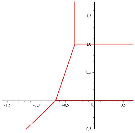
The second dual variety $X_{\mathcal{A}}^{(2)}\subset(\mathbb{P}^{9})^{\vee}$ has the expected dimension $2+9-5=6$ . In this small case, we can compute its ideal $I$ using any Computer Algebra System. Using Singular [6], we found for instance the following polynomial $h\in I$ :

h\,=\,4x_{6}x_{7}^{2}-4x_{5}x_{7}x_{8}+4x_{4}x_{8}^{2}+3x_{5}^{2}x_{9}-12x_{4}x_{6}x_{9}.

The $u$ -weights of the five monomials in $h$ are respectively equal to $(2+2,1+1+1,1+2,2+1,1+1+1)$ . We thus check that ${\rm in}_{u}(h)=-4x_{5}x_{7}x_{8}+4x_{4}x_{8}^{2}+3x_{5}^{2}x_{9}$ is not a monomial, as predicted. However, note that in cases where the ideal cannot be computed, we can still determine (via Theorems 5.3 and 5.6) all weights in the tropicalization.

Acknowledgements: We are grateful to the Royal Institute of Technology and to the Centre of Mathematics for Applications at the University of Oslo, which hosted several of our first discussions, and to the Institut Mittag-Leffler, where the main part of this work was completed. We thank the Göran Gustafsson Foundation for providing financial support for our stays in Stockholm. We thank the referee for a careful reading of our manuscript and for pointing out several typos in the formulas. We also thank Christian Jürgens for the correction of a statement in our previous version.

References

[1] Th. Bauer, S. D. Rocco, and T. Szemberg (2000) Generation of jets on $K3$ surfaces. J. Pure Appl. Algebra 146 (1), pp. 17–27. Cited by: §2.
[2] M. Beltrametti and A. Sommese (1995) The adjunction theory of complex projective varieties. de Gruyter Expositions in Mathematics, Vol. 16, Walter de Gruyter & Co.. External Links: ISBN 3-11-014355-0, Review MathReviews Cited by: §3.2.
[3] R. Bieri and J. Groves (1984) The geometry of the set of characters induced by valuations. J. reine angew. Math. 347, pp. 168–195. Cited by: §1, §5.1.
[4] C. Casagrande and S. D. Rocco (2008) Projective q-factorial toric varieties covered by lines. Comm. Contemp. Math. 10 (3), pp. 363–389. Cited by: §1.
[5] V. I. Danilov (1978) The geometry of toric varieties. Uspekhi Mat. Nauk 33 (2(200)), pp. 85–134, 247. External Links: ISSN 0042-1316 Cited by: §3.1, §3.2, Remark 3.5.
[6] W. Decker, G.-M. Greuel, G. Pfister, and H. Schönemann (2011) Singular 3-1-3 — A computer algebra system for polynomial computations. Note: http://www.singular.uni-kl.de Cited by: Example 5.8.
[7] M. Demazure () Sous-groupes algébriques de rang maximum du groupe de cremona. Ann. Sci. École Norm. Sup. 3 (4), pp. 507–588. Cited by: §3.2, Remark 3.5.
[8] A. Dickenstein, E.M. Feichtner, and B. Sturmfels (2007) Tropical discriminants. J. Amer. Math. Soc. 20 (4), pp. 1111–1133 (electronic). Cited by: §1, §1, §4, §5.3, §5.3, Remark 5.5, Remark 5.5, §5.
[9] A. Dickenstein and L. F. Tabera (2012) Singular tropical hypersurfaces. Discrete and Computational Geometry 47 (2), pp. 430–453. Cited by: §1, §5.3, §5.3, §5.3, §5.3, §5.
[10] L. Ein (1985) Varieties with small dual varieties. II. Duke Math. J. 52 (4), pp. 895–907. Cited by: §1.
[11] L. Ein (1986) Varieties with small dual varieties. I. Invent. Math. 86 (1), pp. 63–74. Cited by: §1.
[12] M. Einsiedler, M. Kapranov, and D. Lind (2006) Non-Archimedean amoebas and tropical varieties. J. Reine Angew. Math. 601, pp. 139–157. Cited by: §5.1.
[13] T. Fujita (1987) On polarized manifolds whose adjoint bundles are not semipositive. 10, pp. 167–178. Cited by: §3.2.
[14] I. M. Gel\cprimefand, M. M. Kapranov, and A. V. Zelevinsky (1994) Discriminants, resultants, and multidimensional determinants. Mathematics: Theory & Applications, Birkhäuser Boston Inc.. External Links: ISBN 0-8176-3660-9 Cited by: §1, §3.1, §5.3.
[15] N. Grigg The tropical maple package. http://math.byu.edu/tropical/maple. Cited by: Figure 1.
[16] A. Lanteri, R. Mallavibarrena, and R. Piene (2008) Inflectional loci of scrolls. Math. Z. 258, pp. 557–564. Cited by: §4, §4, §4.
[17] A. Lanteri, R. Mallavibarrena, and R. Piene (to appear.) Inflectional loci of scrolls over smooth projective varieties. Indiana Univ. Math. J.. Cited by: §4.
[18] A. Lanteri and R. Mallavibarrena (1999) Higher order dual varieties of projective surfaces. Comm. Alg. 27 (10), pp. 4827–4851. Cited by: §2, §2, Remark 3.5.
[19] A. Lanteri and R. Mallavibarrena (2001) Osculatory behavior and second dual varieties of del pezzo surfaces. Adv. Geom. 1 (4), pp. 345–363. Cited by: §1.
[20] R. Mallavibarrena and R. Piene (1991) Duality for elliptic normal surface scrolls. Enumerative algebraic geometry (Copenhagen, 1989). Contemp. Math. 123, pp. 149–160. Cited by: §1.
[21] Y. Matsui and K. Takeuchi (2011) A geometric degree formula for $A$ -discriminants and euler obstructions of toric varieties. Adv. Math. 226 (2), pp. 2040–2064. Cited by: §3.1, §4.
[22] M. Mustaţă (2002) Vanishing theorems on toric varieties. Tohoku Math. J. 54, pp. 451–470. Cited by: Remark 3.4.
[23] R. Piene and G. Sacchiero (1984) Duality for rational normal scrolls. Comm. Algebra 12 (9–10), pp. 1041–1066. Cited by: §1, §3.2, §4, §4, §4, §4.
[24] R. Piene A note on higher order dual varieties, with an application to scrolls. In Singularities, Part 2, (Arcata, Calif., 1981), 335–342, Proc. Sympos. Pure Math., 40, Amer. Math. Soc., Providence, RI, 1983. Cited by: §1.
[25] F. Rincón Computing tropical linear spaces. to appear: Journal of Symbolic Computation, 2012. Software TropLi available at: http://math.berkeley.edu/ felipe/tropli/. Cited by: Remark 5.5, Remark 5.5.
[26] S. D. Rocco, C. Haase, B. Nill, and A. Paffenholz Polyhedral adjunction theory. arXiv:1105.2415. Cited by: §3.2, §3.2.
[27] S. D. Rocco (1999) Generation of $k$ -jets on toric varieties. Math. Z. 231 (1), pp. 169–188. Cited by: §2, §3.1.
[28] S. D. Rocco (2006) Projective duality of toric manifolds and defect polytopes. Proc. London Math. Soc. 93 (3), pp. 197–219. Cited by: §1, §3.1.
[29] B. Sturmfels (2002) Solving systems of polynomial equations. CBMS, Vol. 97, Amer. Math. Soc.. Cited by: Remark 5.5, §5.
[30] J. Tevelev (2007) Compactifications of subvarieties of tori. Amer. J. Math. 129 (4), pp. 1087–1104. Cited by: §5.1.