Naturalness, Supersymmetry and Implications for LHC and Dark Matter

Several naturalness, hierarchy, and, fine-tuning problems exist in particle physics: some big and some small. The most severe one relates to the smallness of the vacuum energy in units of the Planck mass, followed by the smallness of the ratio $M_{W}/M_{\rm Pl}$. There are several other small-to-moderate size hierarchies such as the ratio $M_{\rm GUT}/M_{\rm Pl}$ and the ratios in the fermion mass spectra such as $m_{u}/m_{t}$. Also, there are hierarchy problems of a more technical nature, such as in the Higgs sector of the standard model, where the Higgs boson mass receives a loop correction which is quadratically dependent on the cutoff. This problem is resolved in supersymmetric models with a cancellation between the fermionic and super-fermionic loops which results in the quadratic dependence on the cutoff being replaced by a logarithmic dependence. A similar problem at a much smaller scale often called the little hierarchy problem appears for supersymmetric models if the scalar masses turn out to be large. In fact, in certain models of soft breaking the scalar masses can get large, as is the case in supergravity grand unified models [1] with hierarchical breaking of supersymmetry [2] and for certain string motivated models [3]. Large scalar masses have also been considered in other contexts [4].

The little hierarchy problem can be simply described as follows: in the radiative electroweak symmetry breaking (REWSB) one has $\frac{1}{2}M_{Z}^{2}\simeq-\mu^{2}-m_{H_{2}}^{2}$ where $\mu$ is the Higgs mixing parameter and $m_{H_{2}}$ is the mass of the Higgs boson that couples to the top quark. Naively $m_{H_{2}}$ gets large as the universal scalar mass $m_{0}$ gets large and a large cancellation is needed between $\mu$ and $m_{H_{2}}$ to get a small $M_{Z}$. A more practical approach is to view the REWSB relation as a determination of $\mu$ which is the view point we adopt here. From this perspective, if $m_{0}$ is large the accessibility of sparticles at the LHC rests on the size of $m_{1/2}$ and $\mu$ and thus a small $\mu$ (and a small $m_{H_{2}}$) is desirable. We note in passing that if $m_{0}$ is indeed large, the LHC would turn into a gaugino factory with the sparticles produced being gluinos [5], charginos and neutralinos (see Sec. V). We also note that this region gives a significant enhancement to proton lifetime [6] because of the smallness of the gaugino masses and relative heaviness of the squark masses.

The question then is how one may achieve a small $\mu$ for the above class of models in the context of radiative electroweak symmetry breaking. The basic mechanism for achieving the above was first realized in [7] (for further works see [8, 9, 10]). In the analysis of [7] it was found that there exist two natural regions of radiative breaking, one where there is an upper bound on the soft parameters $m_{0}$, $m_{1/2}$, $A_{0}$ for a fixed $\mu$ (the Ellipsoidal Branch, EB), and the other where one or more soft parameters can get very large for fixed $\mu$ (the Hyperbolic Branch, HB). In a later work, [11], it was shown that there exists a region where the value of the Higgs mass squared, $m_{H_{2}}^{2}$, becomes essentially independent of the values of the input parameter $m_{0}$ at the GUT scale. Such a region was then labeled the Focus Point.

In this work we classify the solutions of the Hyperbolic Branch in Sec. II and show that it contains three main regions: (1) Focal Points (HB/FP): This region lies at the boundary between the Ellipsoidal and the Hyperbolic Branches where $\mu^{2}$ becomes independent of $m_{0}^{2}$ and thus $m_{0}$ can get large while $\mu$ remains fixed with the other soft parameters being held fixed. In this definition we do not include the Focal Point on the EB. The Focal Point is technically different from the Focus Point [11] but for $\tan\beta\gg 1$ they are essentially the same as will be made clear in Sec. II and Sec. III. The HB/FP region, however, is only a small part of HB and the larger parts of HB are Focal Curves and Focal Surfaces as discussed below, and in detail in Sec. II and Sec. IV. (2) Focal Curves (HB/FC): Focal Curves are where two soft parameters are comparable and can get large while $\mu$ is fixed. We define HB/FC such that the HB/FP region is excluded. (3) Focal Surfaces (HB/FS): Here one may have a fixed (and small) $\mu$ while the three dimensional soft parameters may get large. The HB/FS region is the set of all Focal Curves and thus does not include the HB/FP region. In Sec. V, we carry out a numerical analysis of the mSUGRA parameter space under all the experimental constrains including the constraint from the recent LHC-7 data and analyze their effects on the HB region. We will show that the combined constraints severely deplete the Focal Point region, while the Focal Curves and thus Focal Surfaces largely remain intact. We also explore implications for SUSY discovery at the LHC and in dark matter searches. Concluding remarks are presented in Sec. VI.

In this section we will discuss in detail the classification of HB into the three broad regions mentioned in the last section. We begin with the equation for the radiative breaking of the electroweak symmetry

where we have $\overline{m}_{H_{i}}^{2}=m_{H_{i}}^{2}+\Sigma_{i}$ and $\Sigma_{i}$ is the contribution arising from the loop corrections to the effective potential for $i=1,2$ [12]. In the analysis here we will focus on the supergravity grand unification model with universal boundary conditions [1, 13, 14] whose soft breaking sector is described by

where $m_{0}$ is the universal scalar mass, $m_{1/2}$ is the universal gaugino mass, $A_{0}$ is the universal trilinear coupling and $\mu$ is the Higgs mixing parameter in the superpotential. The model of Eq. (2) is referred to as mSUGRA or sometimes as the constrained minimal supersymmetric model, CMSSM. The analysis is done using the techniques given in [15] where one starts with universal boundary conditions given by Eq. (2) for the soft parameters at the GUT scale and evolves the sparticle masses downwards using renormalization group equations. For illustration in the text, we consider one loop evolution where we neglect the Yukawa couplings except for the top quark. The simulations presented later are done using numerical codes which include the effects of the $b$ and $\tau$ Yukawa couplings. As discussed in Sec. I, the radiative electroweak symmetry breaking allows for a determination of $\mu^{2}$ in terms of the soft parameters as [16, 7]

where

and $e.f,g,k$ are as defined in [17]. $D_{0}(t)$ is defined by

Here $Y_{0}=h_{t}(0)^{2}/(4\pi^{2})$, where $h_{t}(0)$ is the top Yukawa coupling at the GUT scale, $M_{G}\simeq 2\times 10^{16}~{\rm GeV}$. Further, $F(t)=\int_{0}^{t}E(t^{\prime})dt^{\prime}~,$ where $E(t)=\left(1+\beta_{3}t\right)^{16/3b_{3}}\left(1+\beta_{2}t\right)^{3/b_{2}}\left(1+\beta_{1}t\right)^{13/9b_{1}}$. Here $\beta_{i}=\alpha_{i}(0)b_{i}/(4\pi)$ and $b_{i}=(-3,1,11)$ for $SU(3),SU(2)$ and $U(1)$ and $t=\ln\left(M_{G}^{2}/Q^{2}\right)$ where $Q$ is the renormalization group point. Our normalizations are such that $\alpha_{3}(0)=\alpha_{2}(0)=\frac{5}{3}\alpha_{1}(0)=\alpha_{G}(0)$. Further, $\Delta\mu^{2}_{\rm loop}$ is the loop correction [12].

As is well known, the tree value of $\mu^{2}$ (Eq. (3) without $\Delta\mu^{2}_{\rm loop}$), is sensitive to the renormalization group scale and the same is true of the loop correction. However, the sum of the tree and the loop term is relatively insensitive to variations in $Q$ [7]. Further, one of the interesting phenomenon observed in [7] is the following: suppose one goes to a renormalization group point $Q$ where the loop contribution $\Delta\mu^{2}_{\rm loop}$ is minimized (this typically occurs at $Q\sim\mathcal{O}\left(\sqrt{M_{\tilde{t}_{1}}M_{\tilde{t}_{2}}}\right)$, where $M_{\tilde{t}_{1}}$ and $M_{\tilde{t}_{2}}$ are the stop masses). Now at low values of $\tan\beta$ and $Q$ it is observed that the co-efficients $C_{i}$ ($i=1-4$) continue to be all positive. In this case it is clear that for any fixed $\mu$ the soft parameters have well defined upper limits. However, for larger values of $\tan\beta$, $C_{1}$ can vanish or even turn negative as $Q$ increases. We will call the region where $C_{1}$ either vanishes or is negative as the Hyperbolic Branch. In this case it is possible to have large soft parameters while $\mu$ remains relatively small.

The HB of REWSB contains three regions: (1) The Focal Point (HB/FP): We define the points where $C_{1}$ vanishes as Focal Points. From Eq. (3) and Eq. (4) we find that when $C_{1}=0$, $m_{0}$ can get large without affecting $\mu$. For practical purposes, for a fixed $\tan\beta$, we will take a small region around $C_{1}=0$, and call it the Focal Point region, specifically

In determining $\delta\left(Q,m_{t}\right)$ we are guided by the experimental error in the top quark mass from $m_{t}=(173.1\pm 1.3)~{\rm GeV}$. Now, for a fixed $\tan\beta$, $C_{1}=C_{1}(m_{t},Q)$ where $Q\sim\mathcal{O}\left(\sqrt{M_{\tilde{t}_{1}}M_{\tilde{t}_{2}}}\right)$ and thus, $Q$ depends on the top mass via the dependence of the stop masses on $m_{t}$. However, this implicit dependence on $m_{t}$ via $Q$ is rather weak and effectively $\delta C_{1}=\frac{\delta C_{1}}{\delta m_{t}}\delta m_{t}$. A direct analysis gives the following approximate result

This result agrees with the one loop analysis in Fig. 1 where $\delta C_{1}$ can be interpreted as the vertical spacing between the curves in the right panel of Fig. 1. In the full numerical analysis presented later in identifying the parameter points that lie in the Focal Point region, we calculate $\delta C_{1}$ numerically for each point by calculating the variation in $C_{1}$ for variations in $m_{t}$. (2) Focal Curves (HB/FC): The region where $C_{1}<0$ allows for two soft parameters to get large while $\mu$ remains small is the Focal Curve region. In fact, in this case there are two general possibilities: HB/FC1 and HB/FC2. In the case of HB/FC1 (HB/FC2), we have $C_{1}<0$ and $m_{1/2}$ ($A_{0}$) as well as $\mu$ are held fixed with $m_{0}$ and $A_{0}$ ($m_{1/2}$) allowed to vary. These two cases can be combined into a single form HB/FC_α defined by $C_{1}<0$ and the constraint $\left(1-\alpha\right)m_{1/2}=\alpha\left|A_{0}\right|$ where $0<\alpha<1$. We note that HB/FC_α reduces to HB/FC1 when $\alpha\sim 0$ and reduces to HB/FC2 when $\alpha\sim 1$. (3) The Focal Surface (HB/FS): is the region of HB where $C_{1}<0$ while all the soft parameters (except $\tan\beta$), i.e, $m_{0},m_{1/2},A_{0}$ vary and may get large while $\mu$ remains fixed. In terms of $\mathrm{HB/FC}_{\alpha}$, varying $\alpha$ creates a Focal Surface.

We discuss now briefly the issue of fine-tuning. Often one uses the criterion of fine-tuning to designate some regions of the parameters as preferred over others. However, such criteria are necessarily subjective and widely different results can be attained by different choices. For example, one criteria used is to look at the sensitivity of $M_{Z}$ to variations in the parameters that enter in Eq. (1). Let us define the set of such parameters to be $a_{i}$, then the sensitivities $f_{i}$ and the fine tuning parameter $f$ are taken to be as in [11]:

(For some early works related to naturalness and fine-tuning see [18, 19, 20, 21, 22] and for more recent works see [23, 24, 25, 26].)

Using the above criteria it has been argued that certain regions of the parameter space (such as when $A_{0}\neq 0$) are less natural than the $A_{0}=0$ region [11]. However, such an argument appears to us as hasty in suppressing parts of the parameter space based purely on a theoretical prejudice. For example, as already noted in [11] inclusion of the top Yukawa in the list $\{a_{i}\}$ would lead to very different conclusions. It may turn out that nature chooses a parameter point which one might consider ‘unnatural’ from a criteria such as of Eq. (11) but is perhaps the natural consequence of a more unified approach. In our analysis we will not rely on criteria such as Eq. (11) as a selection principle for the parameter space. Such criteria are subjective and thus weaker. Rather, we take the more pragmatic approach regarding exploration of the entire parameter from a phenomenologically desirable view point. Such a view point requires that we explore the small $\mu$ region of the parameter space while one or more of the other soft parameters (such as $m_{0}$ and $A_{0}$) could become large. Effectively our naturalness criteria will be simply regions of small $\mu$ as in the analysis of [7]. Thus solutions of this type appear desirable for phenomenological reasons regarding the detectability of new physics at the LHC. Further, as mentioned earlier situations of this type arise in theory models [2, 3].

While the Hyperbolic Branch [7] and the Focus Point [11] both allow for large values of $m_{0}$ while $\mu$ remains small, the exact relationship of the Hyperbolic Branch and of the Focus Point has not been elucidated in the literature. In this section we establish a direct connection between the two. We show that the Focus Point is the boundary point of a Focal Curve on the Hyperbolic Branch. Again for illustration we will consider one loop evolution, and among the Yukawa couplings retain only the top quark coupling. Here the scalar masses $m_{H_{2}}^{2}$, $m_{\tilde{U}}^{2}$ and $m_{\tilde{Q}}^{2}$ satisfy the following set of coupled equations

where $\Sigma=(m_{H_{2}}^{2}+m_{\tilde{Q}}^{2}+m_{\tilde{U}}^{2})$, $Y_{t}=h_{t}^{2}/(16\pi^{2})$, and where $h_{t}$ is the Yukawa coupling at scale $Q$. The analysis of [11] made the observation that the solution to Eq. (12), can be written in the form $m_{i}^{2}=(m_{i}^{2})_{p}+\delta m_{i}^{2}$ where $(m_{i}^{2})_{p}$ is the particular solution and the $\delta m_{i}^{2}$ obey the homogeneous equation

The solution to the above with the universal boundary conditions at the GUT scale is given by

where $J$ is an integration factor defined by

As $Q\to M_{G}$, one has $J(t)\to 1$ and the universality of the masses is recovered at the GUT scale. Noting that $Y(t)$ at the one loop level satisfies the equation

one finds $Y_{t}$ so that

where $F(t)$ and $E(t)$ are defined after Eq. (8), one can inspect $J(t)$ to find that $J(t)=D_{0}(t)$, where $D_{0}(t)$ is defined by Eq. (8). Thus $\delta m^{2}_{H_{2}}$ takes the form

and $C_{1}$ can be expressed in terms of $\delta\overline{m}_{H_{2}}^{2}$

From Eq. (33) we see that the correction $\delta m^{2}_{H_{2}}$ becomes independent of $m_{0}$ when $D_{0}=1/3$, which corresponds to the so called Focus Point region [11], and from Eq. (34) one finds that $\delta\overline{m}_{H_{2}}^{2}\to 0$ implies that $C_{1}$ also vanishes, for $\tan\beta\gg 1$. Thus for large $\tan\beta$, i.e. $\tan\beta\gtrsim 5$, the Focal Point and the Focus Point essentially merge. More explicitly, the Focus Point implies the vanishing of $\delta\overline{m}_{H_{2}}^{2}$ while the Focal Point requires the vanishing of $C_{1}$. A numerical analysis of the behavior of $C_{1}$ as a function of $Q$ for a set of fixed $\tan\beta$’s is given in Fig. 1 as well as a graphical representation of the different branches. Fig. 1 shows that the Focal Point is the boundary point of HB or, in other words, the transition point between EB and HB.

Focal  Curves (HB/FC): To exhibit the emergence of a Focal Curve we rewrite Eq. (1) in the following form

Now, suppose we go to the renormalization group point $Q$ where the loop corrections are minimized and, further, we are in a region of $\tan\beta$ and $Q$ where $C_{1}$ is negative. In this case one finds that there exist curves where $m_{0}$ and $A_{0}$ get large while $m_{1/2}$ is held fixed and $\mu$ is relatively small compared to $m_{0}$ and $A_{0}$. Thus we can rewrite Eq. (35) in the form

where $\pm|\mu_{1}|^{2}\equiv\mu^{2}+\frac{1}{2}M_{Z}^{2}-m_{1/2}^{2}\overline{C}_{3}-\Delta\mu^{2}_{\rm loop}$ , where $\pm$ indicates the overall sign of the right hand side. Thus one has two branches corresponding to the two signs. We can interpret Eq. (37) as an equation of a Focal Curve in the $m_{0}-\bar{A}_{0}$ plane (or in the $m_{0}-A_{0}$ plane around a shifted origin in $A_{0}$) such that as $m_{0}$ and $A_{0}$ get large, $\mu$ remains fixed for fixed $m_{1/2}$ (this is Focal Curve HB/FC1 as defined in Sec. II). In the limit when $m_{0},|A_{0}|$ (and $Q$) are much larger than $\mu$ and $m_{1/2}$ one gets the result

where the last entry in Eq. (38) arises from a numerical evaluation of $C_{1}$ and $C_{2}$ as given by Eq. (4) and Eq. (5) as shown in Fig. 2.

In order to identify which points lie on Focal Curves we compute the $C_{i}$ for each point and then subject them to the conditions necessary for them to lie on a Focal Curve. Thus for the case presented above we consider $m_{1/2}$ fixed while $m_{0}$ and $A_{0}$ vary with $C_{1}<0$ and outside the Focal Point region. An analysis illustrating Focal Curves in this case is given in Table 1. For this analysis and subsequent figures and tables we use both SuSpect [27] and SoftSUSY [28] which include the two loop renormalization group equations and the two loop corrections to the Higgs sector. The analysis is done for the case when $m_{0}$ lies in the range $500~{\rm GeV}$ to $4000~{\rm GeV}$ and $A_{0}$ lies in the range $-500~{\rm GeV}$ to $-3000~{\rm GeV}$ with $\tan\beta=15$ and $\mu$ remaining within $10\%$ of $600~{\rm GeV}$. A similar analysis is shown pictorially in the left panel of Fig. 3, where we have displayed the Focal Curves for $m_{1/2}=500~{\rm GeV}$, $\tan\beta=45$ and $\mu=\left(465\pm 35\right)~{\rm GeV}$. We see that for $m_{0}$ and $|A_{0}|$ large, there is good agreement with Eq. (38), i.e., one finds $A_{0}/m_{0}\to\pm 1$ asymptotically for large $m_{0}$. We note that the limit $A_{0}/m_{0}\sim 1$ consistent with small $\mu$ was noticed and discussed recently in the analysis of [24] in the context of a string motivated model. From the left panel of Fig. 3 we note that this limit is part of HB and is specifically the end point of the Focal Curve HB/FC1. The left panel of Fig. 4 shows model points with $m_{1/2}<1~{\rm TeV}$ and $m_{0}>10~{\rm TeV}$ with $\mu<2~{\rm TeV}$. The result of $m_{0}$ up to $10~{\rm TeV}$ were exhibited in [7], and up to $30~{\rm TeV}$ in [24], and here we exhibit $m_{0}$ up to $50~{\rm TeV}$ and beyond for $\mu<2~{\rm TeV}$, i.e., $\mu/m_{0}\ll 1$.

Now there is also another possibility of achieving a Focal Curve which can be illustrated by writing Eq. (3) in the form

As before, we can write this equation in the form

where $\pm|\mu_{2}|^{2}\equiv\mu^{2}+\frac{1}{2}M_{Z}^{2}-A_{0}^{2}\overline{C}_{2}-\Delta\mu^{2}_{\rm loop}$ . Thus again one has two branches depending on the sign. Here one keeps $A_{0}$ fixed while $m_{0}$ and $m_{1/2}$ get large and $\mu$ is relatively small (this is Focal Curve HB/FC2 as defined in Sec. II). For the case when $|\mu_{2}|$ is small relative to $m_{0}$ and $\overline{m}_{1/2}$ one finds the following relationship asymptotically

where the last entry in Eq. (42) is obtained by using Eq. (4) and Eq. (6) as shown in Fig. 2. An illustration of this case is given in the right panel of Fig. 3 where $m_{1/2}$ gets very large. For these curves we see that we can still have models with $\mu$ small ($\mu\lesssim 450~{\rm GeV}$) and $m_{1/2}$ large ($m_{1/2}\gtrsim 1500~{\rm GeV}$), which leads to the gluino mass being on the order of a few TeV or larger.

To show that there exists a larger set of Focal Curves than the cases we have discussed above we exhibit a whole set of parametric Focal Curves which we label as HB/FC_α. To do this we define $\left(1-\alpha\right)m_{1/2}=\alpha|A_{0}|$, where $0<\alpha<1$. This allows us to rewrite Eq. (3) as

where $\pm|\mu_{\alpha}|^{2}=\mu^{2}+\frac{1}{2}M_{Z}^{2}-\Delta\mu_{\rm loop}^{2}$. Further,

Eq. (43) shows that there exists parametric Focal Curves, parameterized by $\alpha$, where one can get the same value of $\mu$ which can be taken to be small, while $\alpha$ can take on values in the range $(0,1)$. This phenomenon illustrated in the right panel of Fig. 4 displays several Focal Curves for constant $\mu$. One finds that as $\alpha$ decreases the asymptotic form of the curves in the $A_{0}-m_{0}$ plane become more steep. This result is in agreement with the theoretical prediction at one loop for the asymptotic ratio $A_{0}/m_{0}$ which is

Focal Surfaces HB/FS: We consider next the radiative breaking of the electroweak symmetry where all the three parameters $m_{0}$, $m_{1/2}$, or $A_{0}$ can get large while $\mu$ remains small. This solution is again valid in the region of the parameter space where $C_{1}$ turns negative at the value of renormalization group point which minimizes the loop correction. This is the Focal Surface HB/FS as defined in Sec. II and we can express it in the following two forms

where $\pm|\mu_{s}|^{2}=\mu^{2}+\frac{1}{2}M_{Z}^{2}-\Delta\mu_{\rm loop}^{2}$. A summary of focal regions is given in Table 2. An exhibition of a Focal Surface for the case $\mu=(0.465\pm 0.035)~{\rm TeV}$ is given in Fig. 5. We note that on the Focal Surface shown in Fig. 5 $m_{0}$, $m_{1/2}$, or $A_{0}$ can all be seen to get large in certain regions while $\mu$ remains relatively constant. We note in passing that another way to generate a Focal Surface is to consider a Focal Curve HB/FC_α and let $\alpha$ vary over its allowed range $0\leq\alpha<1$. Thus a Focal Surface can be viewed as a collection of Focal Curves as in the right panel of Fig. 4.

Constraints of LHC-7 data on Focal Regions: We now investigate the implications of the recent LHC data [29, 30, 31, 32, 33] on the focal regions constituted of the Focal Point, Focal Curves and Focal Surfaces. To this end we first generate mSUGRA parameter points using a uniformly distributed random scan over the soft parameters with $m_{0}<4~{\rm TeV}$, $m_{1/2}<2~{\rm TeV}$, $A_{0}/m_{0}\in(-10,10)$, and $\tan\beta\in(1,60)$. After the constraint of REWSB roughly 22 million mSUGRA parameter points are collected. These are then subject to experimental constraints which include the LEP and Tevatron [34] limits on the Higgs mass and on the sparticle masses as discussed in [35, 36] and ${\mathcal{B}r}\left(B_{s}\to\mu^{+}\mu^{-}\right)\leq 1.1\times 10^{-8}$ [37]. These constraints will be referred to as the general constraints. In imposing these constraints we use MicrOMEGAs [38] for the computation of the relic density and SuSpect for the computation of the sparticle mass spectrum and $\mu$ at the scale at which electroweak symmetry breaks, $Q_{\rm EWSB}$. A more statistically rigorous procedure for the implementation of the constraints would be to use $\chi^{2}$ or maximum likelihoods, but for the purpose of this analysis it is unnecessary.

CMS and ATLAS have reported results for supersymmetry searches [29, 30, 31, 32, 33] based on about $1~\mathrm{fb}^{-1}$ of data. The implications of these results (as well as dark matter results) have been considered for the parameter space of SUSY models in a number of works [39, 40, 41, 42, 35, 43] and some discussion on the collider implications on naturalness can be found in [44, 45, 46, 47]. Here we use the constraint arising from the recent ATLAS $1~\mathrm{fb}^{-1}$ search [33] and the CMS $1~\mathrm{fb}^{-1}$ search [29] to explore their implications on the focal region. The implications of the LHC data for the Ellipsoidal Branch and for the Hyperbolic Branch are exhibited in Fig. 6. The top left panel gives the parameter space in EB and here one finds that most of the model points being constrained by LHC-7 lie in the low $m_{0}$ region. The top right panel gives the corresponding analysis for HB/FP and HB/FC. In the analysis here we have assumed that $m_{1/2}/m_{0}\leq 0.1$ for HB/FC1 and $A_{0}/m_{0}\leq 0.1$ for HB/FC2. The middle left panel exhibits the same set of parameter points on HB/FP and HB/FC as the top left panel except that the regions are now labeled according to the sparticle landscape picture [48] by the next to lightest particle beyond the Standard Model (NLP) in the mass hierarchy (note that this includes all of the sparticles and Higgs sector particles, but omits the Standard Model-like $h^{0}$). Here one finds that most of the region being constrained by the LHC-7 data is the high $m_{0}$ region. The middle right panel exhibits the Focal Point region, HB/FP. Here one finds that the Focal Point region HB/FP is highly depleted and is further constrained by the LHC-7 data. The bottom panels of Fig. 6 show the parameter points on HB/FS which is the entire HB region except the HB/FP region. The left panel displays the parameter points where the NLP is either a $\tilde{\chi}^{\pm}_{1}$ or $\tilde{\tau}_{1}$, and the right hand panel shows the parameter points where the NLP is $\tilde{t},A$ or $H$. Thus the analysis of Fig. 6 shows that the HB/FP is almost empty and most of the parameter space remaining on HB lies in the region of Focal Curves or Focal Surfaces, i.e., it lies on HB/FC and HB/FS.

LHC signals on HB/FC1: We discuss now an important phenomenon related to HB/FC1, which arises from the constraint that $m_{1/2}$ and $\mu$ are fixed even though $A_{0}$ and $m_{0}$ get large. This can lead to observable leptonic signatures, specifically the trileptonic signature [49, 50], even when $m_{0}$ lies in the several TeV region (For a recent work on the trileptonic signal see [51]). The reason for this is rather obvious, in that the chargino and the neutralino masses are held relatively constant along the Focal Curve HB/FC1. Thus the production cross-section for the charginos and neutralinos will be essentially independent of $m_{0}$. We are specifically interested in the production cross-section of the light chargino $\tilde{\chi}^{\pm}_{1}$ and the second lightest neutralino $\tilde{\chi}^{0}_{2}$, i.e., $\sigma_{\tilde{\chi}^{\pm}_{1}\tilde{\chi}^{0}_{2}}$ which can lead to a trileptonic signal from the decay of $\tilde{\chi}^{\pm}_{1},\tilde{\chi}^{0}_{2}$ so that $\tilde{\chi}^{\pm}_{1}\to l^{\pm}+\nu_{l}+\tilde{\chi}^{0}_{1}$ and $\tilde{\chi}^{0}_{2}\to l^{+}l^{-}\tilde{\chi}^{0}_{1}$ (important contributions can also arise from the production of $\tilde{\chi}^{\pm}_{1}\tilde{\chi}^{0}_{i}$ (i=3,4) depending on the part of the parameter space one is in). The chargino and neutralino final state can arise at tree level from two main processes in $pp$ collisions. Thus, for example, $\tilde{\chi}^{+}_{a}\tilde{\chi}^{0}_{i}$ can arise from the s-channel fusion diagram $u+\bar{d}\to W^{+*}\to\tilde{\chi}^{+}_{a}+\tilde{\chi}^{0}_{i}$ and from the t-channel exchange diagram of a $\tilde{d}_{L}$ squark. The latter diagram is suppressed when $m_{0}$ is large so that the main production cross-section proceeds via the s-channel off -shell $W^{\pm}$ production [50]. Thus the $\tilde{\chi}^{\pm}_{1}\tilde{\chi}^{0}_{i}$ production cross-section is expected to be independent of $m_{0}$ for large $m_{0}$. The constancy of $\sigma_{\tilde{\chi}^{\pm}_{1}\tilde{\chi}^{0}_{2}}/\sigma_{\rm total}$ is exhibited in Fig. 7 for HB/FC1 defined by $m_{1/2}=0.35~{\rm TeV}$, $\tan\beta=45$ and $\mu=(0.20\pm 0.01)~{\rm TeV}$. The branching ratio into trileptons is also computed. In the analysis we use SUSY-HIT [52] for the computation of decays, PYTHIA [53] for event generation, and PGS [54] for detector simulation. For the case of models exhibited in Fig. 7 the $\tilde{\chi}^{\pm}_{1}\tilde{\chi}^{0}_{2}$ production cross-section is $\left(164.3\pm 9.97\right)~{\rm fb}$ and the $\tilde{\chi}^{\pm}_{1}\tilde{\chi}^{0}_{3}$ production cross-section is $\left(112.1\pm 8.53\right)~{\rm fb}$, which leads to roughly $50$ raw trilepton events at $10~\mathrm{fb}^{-1}$ where we have included $\tau$s in the definition of leptons. The number of events will be reduced when off-line cuts are imposed and a more detailed analysis would require further knowledge of the cuts used in the experimental multileptonic search at that luminosity. Of course a much larger number of events is expected at higher $\sqrt{s}=10~{\rm TeV}$, or $\sqrt{s}=14~{\rm TeV}$ at the same luminosity. Similarly, the $\tilde{\chi}^{\pm}_{1}\tilde{\chi}^{0}_{2}$ and $\tilde{\chi}^{\pm}_{1}\tilde{\chi}^{0}_{3}$ production states can decay hadronically. For the hadronic analysis we use the cuts as outlined in Ref. 1 of [33] by ATLAS and find that our effective cross-sections are $\left(5.2\pm 0.15\right)~{\rm fb}$, $\left(0.7\pm 0.16\right)~{\rm fb}$, $\left(1.6\pm 0.33\right)~{\rm fb}$, $\left(0.6\pm 0.18\right)~{\rm fb}$ and $\left(0.5\pm 0.15\right)~{\rm fb}$ which can be compared to the reported $95\%$ C.L. upper bounds at $1.04~\mathrm{fb}^{-1}$ of $22~{\rm fb}$, $25~{\rm fb}$, $429~{\rm fb}$, $27~{\rm fb}$ and $17~{\rm fb}$, respectively. Typically these points produce hard jet signatures, but with low jet multiplicity. Thus the hadronic signals on HB/FC1 may become visible if a luminosity in excess of $20~\mathrm{fb}^{-1}$ can be achieved at LHC-7. Another possible channel for discovery would be a combination of jets and leptons, but such an analysis is outside the scope of the current work.

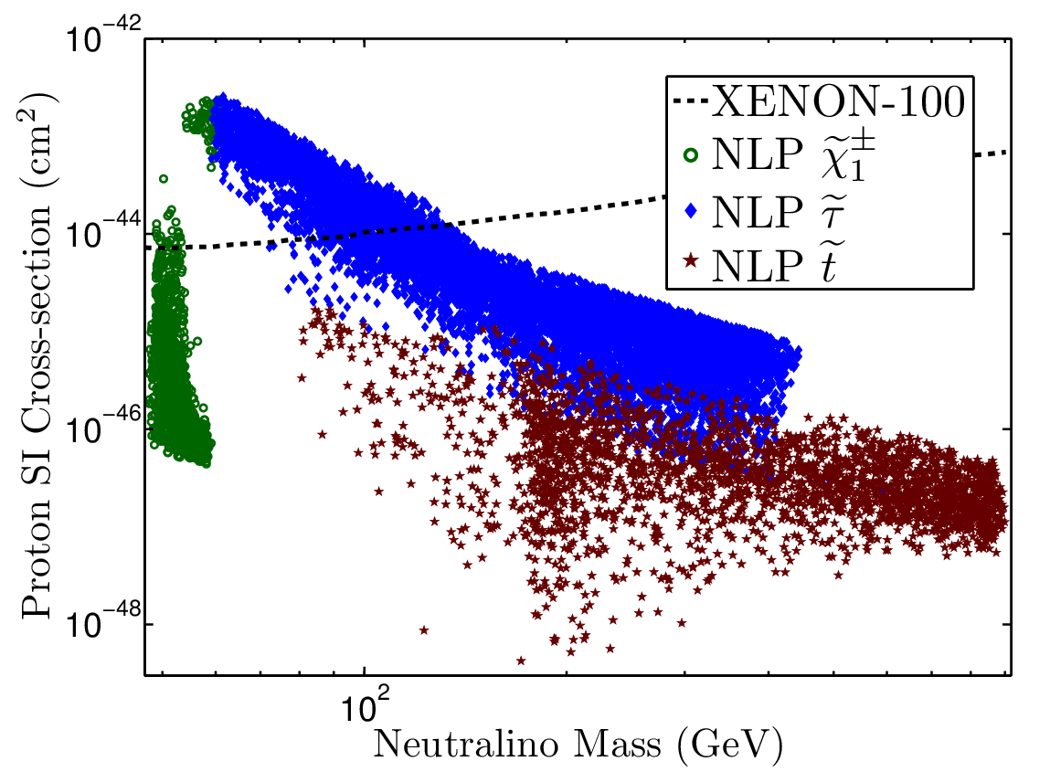
Dark Matter in the EB and the Focal Domains: It is interesting to investigate the prediction for dark matter searches in EB vs HB domains. We begin by considering first the full parameter space of mSUGRA which, after general constraints, is exhibited in the top left panel of Fig. 8 where the LHC-7 constraint with $1~\mathrm{fb}^{-1}$ of data is also exhibited. The spin-independent cross-section vs the neutralino mass corresponding to the parameter space in the top left panel is exhibited in the top right panel where we have also exhibited the experimental exclusion from XENON-100 experiment. Next, in the bottom left panel of Fig. 8, we exhibit the spin-independent neutralino-proton cross-section vs the neutralino mass for EB while the bottom right panel exhibits the same for the full HB domain consisting of HB/FP, HB/FC and HB/FS. The HB/FP region indicated by the red area is rather small while most of the remaining parameter space is constituted of HB/FC and HB/FS.

It is shown that the Hyperbolic Branch of radiative electroweak symmetry breaking consists of several regions of the parameter space where $\mu$ is small. These regions consist of the Focal Points, Focal Curves and Focal Surfaces. The Focal Point (HB/FP) region is where $m_{0}$ can get large with fixed $m_{1/2}$ and $A_{0}$ while $\mu$ remains small. A small $\mu$ can also be achieved on Focal Curves and on Focal Surfaces. There are two possible Focal Curves: HB/FC1 and HB/FC2 such that on HB/FC1, $m_{0}$ and $A_{0}$ both may get large, while $m_{1/2}$ and $\mu$ remain fixed, while on HB/FC2, $m_{0}$ and $m_{1/2}$ may get large while $A_{0}$ remains fixed. These two general categories can be unified by the parameter $\alpha$ defining the Focal Curve mode $\mathrm{HB/FC}_{\alpha}$. An explicit illustration of these regions is given for mSUGRA where it is shown that the HB/FP region is significantly depleted when all the experimental constrains along with the current constraints from the LHC-7 data are applied. Thus the remaining parameter points in this region lie on Focal Curves (or more generally, on Focal Surfaces). Thus if $m_{0}$ is indeed large while the gaugino masses are light, the LHC would turn into a gaugino factory. Some of the SUSY signals for this case were also discussed.