![[Uncaptioned image]](1111.4497v1/logos.png)
Study of Inclusive Jet Production and Jet Shapes in proton-proton collisions at TeV using the ATLAS Detector11
1
Ph.D. Dissertation
Francesc Vives Vaqué
Institut de Física d’Altes Energies
Universitat Autònoma de Barcelona
Departament de Física
Edifici Cn, Campus UAB
E-08193 Bellaterra (Barcelona)
Barcelona, July 2011
supervised by
Prof. Mario Martínez Pérez
ICREA / Institut de Física d’Altes Energies /
Universitat Autònoma de Barcelona
The studies presented in this thesis are part of the following publications:
- •
The ATLAS Collaboration, Study of jet shapes in inclusive jet production in collisions at TeV using the ATLAS detector, Physical Review D 83, 052003 (2011)
- •
The ATLAS Collaboration, Measurement of inclusive jet and dijet cross sections in proton-proton collisions at 7 TeV centre-of-mass energy with the ATLAS detector, European Physical Journal C71 1512 (2011)
and of the following public ATLAS notes:
- •
The ATLAS Collaboration, Jet Shapes in ATLAS and Monte Carlo modeling, ATL-PUB-2011-010 (2011)
- •
The ATLAS Collaboration, Measurement of inclusive jet and dijet cross sections in proton-proton collision data at 7 TeV centre-of-mass energy using the ATLAS detector, ATLAS-CONF-2011-047 (2011)
- •
The ATLAS Collaboration, Properties and internal structure of jets produced in soft proton-proton collisions at GeV, ATLAS-CONF-2010-018 (2010)
Acknowledgments
First of all, I would like to thank my supervisor Mario Martínez. His broad knowledge of physics, involvement in the analysis I was performing and love for rigorous work have played a crucial role in this thesis. I am grateful to Enrique Férnandez, Matteo Cavalli and Martine Bosman, who welcomed me at IFAE, and from whom I admire their passion for physics.
I also want to thank the ATLAS collaboration. In particular, I want to mention Fabiola Gianotti, the spokesperson, Kevin Einsweiler and Jon Butterworth, the Standard Model group conveners, and Tancredi Carli and Richard Teuscher, conveners of the Jet/EtMiss group.
I started the jet shapes analysis with Monica D’Onofrio. I would like to thank her for this collaboration, but mainly for her multiple advises and friendship. Other postdocs have helped me during my Ph.D., and I am grateful to all of them: Bilge Demirköz, with whom I analyzed the first ATLAS data, Christophe Ochando, Ilya Korolkov, Luca Fiorini and Sebastian Grinstein.
Estel, Evelin and Valerio have been excellent office-mates, and actually more than that. Just to put an example, they were the first friends to visit my daughter Gemma when she was born! I also want to thank my other colleagues at IFAE, in particular Machi, Jordi and Volker.
I am grateful to Juan and Sonia, for their encouragement during the Ph.D., and to all my friends working at CERN: Ila, Peppe, Alessio, Ciccio, Simone, Lidia, Delo, Paola…
Finally, I want to thank the most important people in my life: my family. I want to particularly mention my wife, Maria Laura, not only for moving to life with me close to CERN, but mainly for her daily support.
Introduction
The Standard Model (SM) is the theory that provides the best description of the properties and interactions of elementary particles. The strong interaction between quarks and gluons is described by the Quantum Chromodynamics (QCD) field theory. Jet production is the high- process with the largest cross section at hadron colliders. The jet cross section measurement is a fundamental test of QCD and it is sensitive to the presence of new physics. It also provides information on the parton distribution functions and the strong coupling. One of the fundamental elements of jet measurements is the proper understanding of the energy flow around the jet core and the validation of the QCD description contained in the event generators, such as parton shower cascades, and the fragmentation and underlying event models. Jet shapes observables are sensitive to these phenomena and thus very adequate to this purpose. The first measurement of the inclusive jet cross section in collisions at TeV delivered by the LHC was done using an integrated luminosity of 17 nb-1 recorded by the ATLAS experiment. The measurement was performed for jets with GeV and , reconstructed with the anti- algorithm with radius parameters and .
This Ph.D. Thesis presents the updated measurement of the inclusive jet cross section using the full 2010 data set, corresponding to 37 pb-1 collected by ATLAS. Jets with GeV and are considered in this analysis. The measurement of the jet shapes using the first 3 pb-1 is also presented, for jets with GeV and . Both measurements are unfolded back to the particle level. The inclusive jet cross section measurement is compared to NLO predictions corrected for non-perturbative effects, and to predictions from an event generator that includes NLO matrix elements. Jet shapes measurements are compared to the predictions from several LO matrix elements event generators.
The contents of this Thesis are organized as follows: Chapter 1 contains a description of the strong interaction theory and jet phenomenology. The LHC collider and the ATLAS experiment are described in Chapter 2. The inclusive jet cross section measurement is described in detail in Chapter 3, and the jet shapes measurements in Chapter 4. Additional comparison of the jet shapes measurement to Monte Carlo event generator predictions are shown in Chapter 5. There are two appendixes at the end of the document. The first one contains additional jet shapes studies, and the second one is devoted to energy flow studies at calorimeter level.
Chapter 1 QCD at Hadron Colliders
1.1 The Standard Model
The Standard Model (SM) [1] is the most successful theory describing the properties and interactions (electromagnetic, weak and strong) of the elementary particles. The SM is a gauge quantum field theory based in the symmetry group , where the electroweak sector is based in the group, and the strong sector is based in the group.
Interactions in the SM occur via the exchange of integer spin bosons. The mediators of the electromagnetic and strong interactions, the photon and eight gluons respectively, are massless. The weak force acts via the exchange of three massive bosons, the and the .
The other elementary particles in the SM are half-integer spin fermions: six quarks and six leptons. Both interact electroweakly, but only quarks feel the strong interaction. Electrons (), muons() and taus() are massive leptons and have electrical charge Q = -1. Their associated neutrinos (, , ) do not have electrical charge. Quarks can be classified in up-type (, , ) and down-type (,,) depending on their electrical charge (Q = 2/3 and Q = -1/3 respectively). For each particle in the SM, there is an anti-particle with opposite quantum numbers.
The SM formalism is written for massless particles and the Higgs mechanism of spontaneous symmetry breaking is proposed for generating non-zero boson and fermion masses. The symmetry breaking requires the introduction of a new field that leads to the existence of a new massive boson, the Higgs boson, that has still not been observed.
1.2 Quantum Chromodynamics Theory
Quantum Chromodynamics (QCD) [2] is the renormalizable gauge field theory that describes the strong interaction between colored particles in the SM. It is based in the symmetric group, and its lagrangian reads:
| (1.1) |
where the sum runs over the six different types of quarks, , that have mass . The field strength tensor, is derived from the gluon field :
| (1.2) |
are the structure constants of , and the indices A, B, C run over the eight color degrees of freedom of the gluon field. The third term originates from the non-abelian character of the group, and is the responsible of the gluon self-interaction, giving rise to triple and quadruple gluon vertexes. This leads to a strong coupling, that is large at low energies and small at high energies (see Figure 1.1). Two consequences follow from this:
- •
Confinement: The color field potential increases linearly with the distance, and therefore quarks and gluons can never be observed as free particles. They are always inside hadrons, either mesons (quark-antiquark) or baryons (three quarks each with a different color). If two quarks separate far enough, the field energy increases and new quarks are created forming colorless hadrons.
- •
Asymptotic freedom: At small distances the strength of the strong coupling is that low that quark and gluons behave as essentially free. This allows to use the perturbative approach in this regime, where .

1.3 Deep inelastic scattering
The scattering of electrons from protons, as illustrated in Figure 1.2, has played a crucial role in the understanding of the proton structure. If the energy of the incoming electron () is low enough, the proton can be considered as a point charge (without structure). The differential cross section with respect to the solid angle of the scattered electron is11 1 The mass of the electron is neglected in all formulas in this Section by assuming .:
| (1.3) |
where () is the fine structure constant, is the angle at which the electron is scattered, is the outgoing electron energy and the mass of the proton. is kinematically determined by .

For higher energies of the incoming electrons, the interaction is sensitive to the proton structure, and the cross section becomes:
| (1.4) |
and are functions that contain information on the proton structure and should be determined experimentally. Given that is kinematically determined by , and only dependent on one variable.

Finally, for even higher electron energies, the proton breaks in a multi-hadron final state as illustrated in Figure 1.3. The cross section is then:
| (1.5) |
Now is the sum of the momenta of the hadrons originating from the proton, and it is not constrained by . Therefore, and are functions of two independent variables, and . Theoretically it is more convenient to use the Lorentz-invariant variables and , where is the momenta of the incoming proton.
The Parton Model describes the proton as built out of three point-like quarks (‘valence quarks’) with spin 1/2, and interprets as the fraction of the proton momentum carried by the quark. From the idea that at high the virtual photon interacts with a quark essentially free, Bjorken predicted that and depend only on at large ( GeV):
| (1.6) |
| (1.7) |
According to the Parton Model:
| (1.8) |
where , called Parton Distribution Function (PDF), is the probability that the th quark carries a fraction of the proton momentum , and is the electrical charge of the quark. Therefore, it is expected that
| (1.9) |
but it was found experimentally that the result of this integral is 0.5. The rest of the proton momentum is carried by gluons. The introduction of gluons leads to a more complex description of the protons structure: quarks radiate gluons, and gluons produce pairs (‘sea quarks’) or radiate other gluons. Figure 1.4 shows the PDFs of the valence quarks of the proton, the gluon, and the sea quarks. The valence quarks dominate at large , whereas the gluon dominates at low .

The radiation of gluons results in a violation of the scaling behavior of and , introducing a logarithmic dependence on , which is experimentally observed (see Figure 1.6). The functional form of the PDFs can not be predicted from pQCD, but it is possible to predict their evolution with .
The parton interactions at first order in are gluon radiation (), gluon splitting () and quark pair production (). The probability that a parton of type radiates a quark or gluon and becomes a parton of type , carrying fraction of the momentum of parton (see Figure 1.5) is given by the splitting functions:

| (1.10) |
| (1.11) |
| (1.12) |
| (1.13) |
The evolution of the PDFs as a function of follow the DGLAP (Dokshitzer, Gribov, Lipatov, Altarelli and Parisi) equations [4]:
| (1.14) |
| (1.15) |
The first equation describes the evolution of the quark PDF with due to gluon radiation and quark pair production, whereas the second equation describes the change of the gluon PDF with due to gluon radiation and gluon splitting. The equations assume massless partons and therefore are only valid for gluons and the light quarks (u, d and s).

1.4 Perturbative QCD
1.4.1 The factorization theorem
The QCD factorization theorem is a crucial concept of QCD, that states that cross sections in hadron-hadron interactions can be separated into a a hard partonic cross section (short-distance) component and a long-distance component, described by universal PDFs:
| (1.16) |
where , are the momenta of the interacting hadrons, the sum runs over all parton types, and is the partonic cross section of the incoming partons with hadron momenta fraction , . is the scale at which the renormalization is performed, and is an arbitrary parameter that separates the hard from the soft component. Both scales are typically chosen to be of the order of .
Partonic cross sections in leading order (LO) calculations for jet production are O(), since they are based on parton interactions (), as shown in Figure 1.7. The dominant process is the scattering because of the larger color charge of the gluons.
Next-to-leading-order (NLO) diagrams include contributions from gluon initial- or final-state radiation and loops on the diagrams already shown. The partonic cross sections at NLO reduce the dependence on the normalization and factorization scales, and are calculable using programs such as JETRAD [5] and NLOJET++ [6]. Predictions at higher orders are not yet available due to the large number of diagrams involved.

1.4.2 Parton Distribution Functions
As already explained, perturbative QCD (pQCD) can predict the evolution of the PDFs [7] with respect to using the DGLAP equations, but not their functional form. Therefore, PDFs should be extracted from experimental data at a given . In particular, seven functions should be determined, one for the gluon and the others for each one of the light quarks and anti-quarks. Experimental data from a large variety of processes is used to constrain several aspects of the PDFs: measurements of Drell-Yan production, inclusive jet cross sections and W-asymmetry in collisions, and deep-inelastic , or scattering.
Typically, specific functional forms are postulated for the PDFs with a set of free parameters. These parameters are obtained optimizing the comparison between experimental data and predictions using the PDFs, for example by minimizing a . The functional form assumed for several sets of PDFs is:
| (1.17) |
where and are the free fit parameters and is a function that tends to a constant in the limits and . This functional form is motivated by counting rules [8] and Regge theory [9], that suggest that and respectively. Both limits are approximate, and even if these theories predict the values of and , they are taken as free fit parameters when computing the PDFs. This approach is used by three of the PDFs used in the analyses presented in this Thesis: CTEQ [10], MSTW [11] and HERA [12] PDFs. For example in the case of HERAPDFs, is:
| (1.18) |
NNPDFs [13] follow a different approach, using neural networks as a parton parametrization. Neural networks are functional forms that can fit a large variety of functions.
1.4.3 Uncertainties
There are three main sources of uncertainties in the calculation of pQCD observables:
- •
The lack of knowledge of higher order terms neglected in the calculation. It is estimated by varying the renormalization scale, , usually by a factor of two with respect to the default choice. The factorization scale, , is independently varied to evaluate the sensitivity to the choice of scale where the PDF evolution is separated from the partonic cross section. The envelope of the variation that these changes introduce in the observable is taken as a systematic uncertainty.
- •
Uncertainties on parameters of the theory, like the and the heavy quark masses, that are propagated into the observable.
- •
PDFs have another uncertainty coming from the way the experimental data is used to determine the PDFs. This uncertainty is typically estimated using the Hessian method. If is the vector of the PDF parameters where is minimized, all parameters such that are considered acceptable fits, where is a parameter called tolerance. PDF parameters are expressed in terms of an orthogonal basis, and variations along the positive and negative directions of each eigenvector (, ) such that are performed. The uncertainty in the observable is:
(1.19) (1.20) where is the observable computed using the PDFs with the parameters in vector . NNPDF use a Monte Carlo approach to evaluate the uncertainties, in which the probability distribution in parameter space derives from a sample of MC replicas of the experimental data. Figure 1.8 shows the PDF of the gluon with its uncertainties obtained following different approaches.

1.5 Monte Carlo simulation
Complete pQCD calculations are always performed only up to a fixed order in , but the enhanced soft-gluon radiation and collinear configurations at higher orders can not be neglected. They are taken into account in the parton shower (PS) approximation, that sum the leading contributions of these topologies to all orders. Monte Carlo (MC) generator programs include the PS approximation, as well as models to reproduce non-perturbative effects, such as the hadronization of the partons to colorless hadrons and the underlying event (UE).
1.5.1 Parton Shower
The PS approximation describes successive parton emission from the partons in the hard interaction, as illustrated in Figure 1.9. The evolution of the showering is governed by DGLAP equations 1.14 and 1.15, from which the Sudakov form factors [14] are derived for the numerical implementation of the parton shower. These factors represent the probability that a parton does not branch between an initial scale () and a lower scale (). Once a branching occurs at a scale , , subsequent branchings are derived from the scales and . They can be angle-, - or -ordered. In the first case subsequent branchings have smaller opening angles than this between and , whereas in the second, parton emissions are produced in decreasing order of intrinsic .

Successive branching stops at a cutoff scale, , of the order of , after producing a high-multiplicity partonic state. Since quark and gluons can not exist isolated, MC programs contain models for the hadronization of the partons into colorless hadrons.
1.5.2 Hadronization
The hypothesis of local parton-hadron duality states that the momentum and quantum numbers of the hadrons follow those of the partons. This hypothesis is the general guide of all hadronization models, but do not give details on the formation of hadrons, that is described in models with parameters that are tuned to experimental data. There are two main models of hadron production.
The string model [16] describes the behavior of pairs using string dynamics. The field between each pair is represented by a string with uniform energy per unit length. As the and the move apart from each other and thus the energy of the color field increases, the string connecting the two is tightened, until it breaks into a new pair. If the invariant mass of either of these string pieces is large enough, further breaks may occur. In the string model, the string break-up process is assumed to proceed until only on-mass-shell hadrons remain. In the simplest approach of baryon production, a diquark is treated just like an ordinary antiquark. A string can break either by quark-antiquark or antidiquark-diquark pair production, leading to three-quark states. There are more sophisticated models, but the formation of baryons is still poorly understood.
The cluster model [17] is based on the confinement property of perturbative QCD, exploited to form color-neutral clusters. After the perturbative parton showering, all gluons are split into light quark-antiquark or diquark-antidiquark pairs. Color-singlet clusters are formed from the quarks and anti-quarks. The clusters thus formed are fragmented into two hadrons. If a cluster is too light to decay into two hadrons, it is taken to represent the lightest single hadron of its flavor. Its mass is shifted to the appropriate value by an exchange of momenta with a neighboring cluster. If the cluster is too heavy, it decays into two clusters, that are further fragmented into hadrons.
1.5.3 Underlying Event
The UE comes from the partons that do not participate in the hard interaction. They contribute to the final state via their color-connection to the hard interaction, and via extra parton-parton interactions. Its simulation is based on the eikonal model, that describes the underlying event activity as additional uncorrelated partonic scatters. The number of interactions per event depends on the impact parameter . A small value corresponds to a large overlap between the two colliding hadrons, and therefore a higher probability for multiple interactions. For a given , the parton-parton cross section is computed as a function of the transverse momentum in the center-of-mass frame of the scattering process . Since this cross section diverges as a cut-off parameter is introduced, where experimentally GeV. is extracted from the ratio between the total hadron cross section and the parton-parton cross section, , and assumed to be Poisson-distributed.
The UE models are tuned using experimental data, such as the jet shapes described in Chapters 4 and 5.
1.5.4 Monte Carlo Generator Programs
PYTHIA Monte Carlo
The PYTHIA [18] MC event generator includes hard processes at LO, and uses the PS model for initial- and final-state radiation. The hadronization is performed using the string model. It includes an underlying event model to describe the interactions between the proton remnants.
The PYTHIA tunes DW [19] and Perugia2010 [20] use CTEQ5L PDFs, and both have been produced using Tevatron data. In the former the PS is -ordered, whereas in the latter it is -ordered.
In autumn 2009, the MRST LO* PDFs [21] were used in PYTHIA for the first time in ATLAS. This required to tune the PYTHIA model parameters, resulting in the MC09 [22] tune. It was done using Tevatron data, mainly from underlying event and minimum bias analyzes. The PS is -ordered.
The PYTHIA-AMBT1 [23] tune followed the MC09 one, and also uses MRST LO* PDFs and -ordered PS. It was derived using ATLAS data, in particular charged particle multiplicities in interactions at 0.9 and 7 TeV center-of-mass energy.
HERWIG
HERWIG [24] is a general-purpose MC event generator for hard processes in particle colliders. It uses an angular-ordered parton-shower for initial- and final-state QCD radiation, and a cluster model to reproduce the hadronization of the partons. The Fortran version of HERWIG is interfaced with JIMMY [25] to simulate multiple parton-parton interactions.
HERWIG++ [26] is the C++ version of HERWIG, that is expected to replace the Fortran one at a given point. The underlying event is modeled inside the program, that therefore do not use JIMMY.
ME + Parton Shower: Alpgen and Powheg
Alpgen [27] is an event generator of multi-parton hard processes in hadronic collisions, that performs the calculation of the exact LO matrix elements for a large set of parton-level processes. It uses the ALPHA algorithm [28] to compute the matrix elements for large parton multiplicities in the final state. The advantage of this algorithm is that its complexity increases slower than the Feynman diagrams approach when increasing the particles in the final state. Powheg [29] is a MC event generator that includes NLO matrix elements. Alpgen and Powheg contain an interface to both PYTHIA and HERWIG for the parton showering, the hadronization and the underlying event simulation.
1.6 Jet Algorithms
Quarks and gluons from the hard scattering result on a collimated flow of particles due to parton shower and hadronization. This collimated flow of particles is called jet. There are several jet definitions [30] with the main purpose of reconstructing jets with kinematics that reflect that of the initial parton. These definitions can be classified in two main types of jet algorithms: cone algorithms and sequential recombination algorithms.
1.6.1 Cone algorithms
Typically, cone jet algorithms start by forming cones of radius in the space around a list of seeds, that can be all particles in the final state or those above a given energy threshold. The center of the cone is recomputed from the particles inside by following either the snowmass or the four-momentum recombination. In the four-momenta recombination, the jet momenta is the sum of the momenta of its constituents:
| (1.21) |
whereas in the snowmass scheme, the jet is considered massless, its transverse energy is the sum of the transverse energy of its constituents and the jet () are the average of the () of the constituents weighted by its transverse energy:
| (1.22) |
| (1.23) |
| (1.24) |
A cone is formed from the new center and the process repeated until the particles inside the cone are no longer changed by further iterations. Usually the algorithm is allowed to form overlapping cones and then decides whether to merge or split them depending on the fraction of energy they share.
This last step makes the cone algorithms collinear or infrared unsafe, and affects the definition of the parton-level jet cross section to all orders in pQCD. A jet algorithm is infrared safe if the addition of an extra particle with infinitesimal energy do not change the jet configuration in the final state. If the replacement of a particle by two collinear particles (which momenta sum is equal to that of the original particle) do not change the jet configuration in the final state, the jet algorithm is collinear safe.
In order to solve this, cone-based jet algorithms have been formulated such that they find all stable cones through some exact procedure, avoiding the use of seeds. These algorithms are very time-consuming from the computational point of view, which constitutes a disadvantage in high-multiplicity events such as those at the LHC.
1.6.2 Sequential recombination jet algorithms
Sequential recombination jet algorithms cluster particles according to their relative transverse momentum, instead of spacial separation. This is motivated by the parton shower evolution as described in Section 1.5.1. For all particles in the final state, the algorithm computes the following distances:
| (1.25) |
| (1.26) |
where is the transverse momentum of particle , between particles and , a parameter of the algorithm that approximately controls the size of the jet, and depends on the jet algorithm: for the algorithm, for the Cambridge/Aachen algorithm, and for the anti- algorithm. The distance is introduced in order to separate particles coming from the hard interaction than those coming from the interaction between remnants. The smallest distance is found, and if it is , particles and are combined into one single object. If instead it is , particle is considered a jet an removed from the list. The distances are recalculated with the remaining objects, and the process repeated until no particle is left in the list. Jets are defined as those objects with above a given threshold.
These algorithms are very convenient, mainly because they are infrared and collinear safe and computationally fast. In particular, the anti- algorithm [31] produces jets with a conical structure in (), as illustrated in Figure 1.10, that facilitates dealing with pile-up. It is the default jet finding algorithm in the LHC experiments.

Chapter 2 The ATLAS Detector at the Large Hadron Collider
The analyses described in this Thesis are performed using proton-proton collision data produced by the Large Hadron Collider (LHC) and collected by the ATLAS detector. In this Chapter, the LHC and the ATLAS detector are described, giving more emphasis to the elements that are relevant for the analyses.
2.1 The Large Hadron Collider
The LHC [32] is a superconducting accelerator built in a circular tunnel of 27 km in circumference that is located at CERN. The tunnel is situated between 45 to 170 m underground, and straddles the Swiss and French borders on the outskirts of Geneva. Two counter rotating proton beams injected into the LHC from the SPS accelerator at 450 GeV are further accelerated to 3.5 TeV while moving around the LHC ring guided by magnets inside a continuous vacuum. During 2010, the instantaneous luminosity was increased over time, with a maximum peak at , and the total integrated luminosity delivered by the LHC was of 48 pb-1 from which ATLAS recorded 45 pb-1 (see Figure 2.1).


There are four main detectors placed along the accelerator line: ATLAS and CMS, that are general-purpose detectors, ALICE, dedicated to heavy-ions physics, and LHCb, dedicated to B-physics.
2.2 The ATLAS experiment
The ATLAS detector [33] is an assembly of several sub-detectors arranged in consecutive layers around the beam axis, as shown in Figure 2.2. The main sub-detectors are the Inner Detector, the Calorimeters and the Muon System, that are described in the next Sections. ATLAS is 46 m long, 25 m wide and 25 m high, and weights 7000 t.
The ATLAS coordinate system and its nomenclature will be used repeatedly throughout this Thesis, and is thus described here. The ATLAS reference system is a Cartesian right-handed coordinate system, with the nominal collision point at the origin. The anti-clockwise beam direction defines the positive -axis, while the positive -axis is defined as pointing from the collision point to the center of the LHC ring and the positive -axis pointing upwards. The azimuthal angle is measured around the beam axis, and the polar angle is measured with respect to the -axis. The pseudorapidity is defined as . The rapidity is defined as , where denotes the energy and is the component of the momentum along the beam direction.
The ATLAS detector was designed to optimize the search for the Higgs boson and a large variety of physics phenomena at the TeV scale proposed by models beyond the Standard Model. The main requirements that follow from these goals are:
- •
Given the high LHC luminosity, detectors require fast, radiation-hard electronics and sensor elements. In addition, high detector granularity is needed to handle the particle fluxes and to reduce the influence of overlapping events.
- •
Large acceptance in pseudorapidity with almost full azimuthal angle coverage.
- •
Good charged-particle momentum resolution and reconstruction efficiency in the inner tracker.
- •
Very good electromagnetic calorimetry for electron and photon identification and measurements, complemented by full-coverage hadronic calorimetry for accurate jet and missing transverse energy measurements.
- •
Good muon identification and momentum resolution over a wide range of momenta and the ability to determine unambiguously the charge of high muons.
- •
Highly efficient triggering on low transverse-momentum objects with sufficient background rejection is a prerequisite to achieve an acceptable trigger rate for most physics processes of interest.

2.3 Inner Detector
The Inner Detector (ID) was designed in order to perform high precision measurements with fine detector granularity in the very large track density events produced by the LHC. The ID, that is m long and 1150 mm in radius, is built out of three components, in increasing order of distance with respect to beam axis: the Pixel detector, the Semiconductor Tracker (SCT) and the Transition Radiation Tracker (TRT). The precision tracking detectors (pixels and SCT) cover the region , and are segmented in and z, whereas the TRT cover the region and is only segmented in . The ID has around 87 million readout channels, 80.4 millions in the pixel detector, 6.3 millions in the SCT and 351 thousand in the TRT. All three are immersed in a 2 T magnetic field generated by the central solenoid, which extends over a length of 5.3 m with a diameter of 2.5 m.
The ID is used to reconstruct tracks and production and decay vertices, and provides a position resolution of 10, 17 and 130 m (Pixel, SCT, TRT) in the plane as well as 115 and 580 m (Pixel, SCT) in the plane. The momentum resolution as a function of of the track is parametrized as:
| (2.1) |
and the values and GeV-1 were determined using cosmic rays [34]. Extrapolation of the fit result yields to a momentum resolution of about 1.6% at low momenta and of about 50% at 1 TeV.
2.4 Calorimeters
The calorimeter systems of ATLAS, illustrated in Figure 2.3 surround the Inner Detector system and cover the full -space and 4.9, extending radially 4.25 m. The calorimeter systems can be classified in electromagnetic calorimeters, designed for precision measurements of electrons and photons, and hadronic calorimeters, that collect the energy from hadrons. Calorimeter cells are pseudo-projective towards the interaction region in . The granularity of the electromagnetic calorimeter is typically in , whereas the hadronic calorimeters have granularity of in most of the regions. The energy response of the calorimeter to single particles is discussed in the next Chapter.

2.4.1 Liquid Argon Calorimeter
The electromagnetic calorimeter is a lead-LAr detector with accordion-shaped kapton electrodes and lead absorber plates over its full coverage. The accordion geometry provides complete symmetry without azimuthal cracks. The calorimeter is divided into a barrel part () and two end-cap components (), each housed in their own cryostat. Over the central region (), the EM calorimeter is segmented in three layers in depth, whereas in the end-cap it is segmented in two sections in depth. Figure 2.4 shows an sketch of a module of the LAr calorimeter.

2.4.2 Hadronic calorimeters
The Tile Calorimeter is placed directly outside the electromagnetic calorimeter envelope. Its barrel covers the region , and its two extended barrels the range . It is a sampling calorimeter using steel as the absorber and scintillating tiles as the active material, and it is segmented in depth in three layers, approximately 1.5, 4.1 and 1.8 interaction lengths () thick for the barrel and 1.5, 2.6, and 3.3 for the extended barrel, as illustrated in Figure 2.5. Two sides of the scintillating tiles are read out by wavelength shifting fibers into two separate photomultiplier tubes.

The Hadronic End-cap Calorimeter (HEC) consists of two independent wheels per end-cap, located directly behind the end-cap electromagnetic calorimeter and sharing the same LAr cryostats. They cover the region , and each wheel is divided into two segments in depth, for a total of four layers per end-cap. The HEC is a sampling calorimeter built out of copper plates intervealed with LAr gaps, that are the active medium.
The Forward Calorimeter (FCal) is integrated into the end-cap cryostats, and it extends in from 3.1 to 4.9. It consists of three modules in each end-cap: the first, made of copper, is optimized for electromagnetic measurements, while the other two, made of tungsten, measure predominantly the energy of hadronic interactions. In all three modules LAr is the sensitive medium.
2.4.3 Calorimeter Topological Clusters
Calorimeter clusters [35] are used as input to the jet finding algorithm in the studies presented in this Thesis. They are built out of neighboring calorimeter cells with significant signal over noise. Therefore, the 3-D shape and the number of cells of clusters are not fixed. The noise is computed for each cell independently, and it is defined as the expected RMS of the electronic noise for the current gain and conditions plus the contribution from pileup added in quadrature.
In order to make clusters, all cells with a signal to noise ratio above 4 are taken as seed cells. These cells are considered in descending order of signal to noise ratio, adding all neighboring cells to them forming the so called proto-clusters. Neighboring cells with signal to noise ratio between 2 and 4 are taken as seed cells in the next iteration. If a cell is adjacent to more than one proto-cluster and its signal to noise ratio is above 2 the proto-clusters are merged, whereas if it is smaller than 2 the cell is only added to the first proto-cluster. Once there are no more cells in the seed list, an splitting algorithm based on local maxima is run over the proto-clusters in order to separate clusters that are not isolated.
Final clusters are treated as massless and their energy, at the electromagnetic (EM) scale, is the sum of the energies of the cells belonging to the cluster. The EM scale is the appropriate scale for the reconstruction of the energy deposited by electrons or photons in the calorimeter. The EM energy scale was first determined using electron test-beam measurements in the barrel and endcap calorimeters [36] [37]. Muons from test-beams and produced in cosmic rays were used to validate the EM scale in the hadronic calorimeter [36] [38]. Recently, a recalibration of the electromagnetic calorimeters has been derived from events in pp collisions. The EM scale uncertainty is 1.5% in the EM LAr barrel calorimeter, and 3% in the Tile calorimeter.
2.5 Muon System
The calorimeter is surrounded by the Muon Spectrometer. The air-core toroid system, with a long barrel and two inserted end-cap magnets, generates a large magnetic field volume with strong bending power within a light and open structure. Multiple-scattering effects are thereby minimized, and excellent muon momentum resolution is achieved with three stations of high-precision tracking chambers. The muon instrumentation includes trigger chambers with very fast time response.
2.6 Luminosity measurement
The luminosity, , of a collider that operates at a revolution frequency and bunches cross at the interaction point can be expressed as
| (2.2) |
where and are the numbers of particles in the two colliding bunches and and characterize the widths of the horizontal and vertical beam profiles, that are measured using van der Meer scans. The observed event rate is recorded while scanning the two beams across each other first in the horizontal (), then in the vertical () direction. This measurement yields two bell-shaped curves, with the maximum rate at zero separation, from which one extracts the values of and . The luminosity at zero separation can then be computed using Equation 2.2.
ATLAS measures the luminosity [39] in inelastic interactions using different detectors and algorithms, all based on event-counting techniques, that is, on determining the fraction of bunch crossings (BCs) during which a specified detector registers an event satisfying a given selection requirement:
| (2.3) |
where is the average number of inelastic interactions per BC, is the inelastic cross section, is the efficiency for one inelastic collision to satisfy the event-selection criteria, and is the averaged number of visible (passing that event selection criteria) inelastic interactions per BC. The visible cross section is the calibration constant that relates the measurable quantity to the luminosity . Both and depend on the pseudorapidity distribution and particle composition of the collision products, and are therefore different for each luminosity detector and algorithm.
In the limit , the average number of visible inelastic interactions per BC is given by the intuitive expression
| (2.4) |
where is the number of events passing the selection criteria that are observed during a given time interval, and is the number of bunch crossings in that same interval. When increases, the probability that two or more interactions occur in the same BC is not negligible, and is no longer linearly related to the raw event count . Instead must be calculated taking into account Poisson statistics, and in some cases, instrumental or pile-up related effects.
can be extracted from Equation 2.3 using the measured values of and , computed with the van der Meer technique, that allows the determination of without a priori knowledge of the inelastic cross section or of detector efficiencies.
2.7 Trigger
The trigger system has three different levels: Level-1 trigger (LVL1), Level-2 trigger (LVL2) and the Event Filter (EF). Each trigger level refines the decisions made at the previous step and, when necessary, applies additional selection criteria. The rate of selected events 11 1 The LHC provides a collision rate of 40 MHz within full operational state. is reduced to around 200 Hz for permanent storage trough the trigger chain, with an event size is approximately 1.3 Mbyte.
The L1 trigger searches for high transverse-momentum muons, electrons, photons, jets, and leptons decaying into hadrons, as well as large missing and total transverse energy. Its selection is based on information from a subset of detectors, and reduces the event rate to about 75 kHz in less than 2.5 s. In each event, the L1 trigger defines one or more regions in and from those regions within the detector where its selection process has identified interesting features. Data in these regions, called Regions-of-Interest (RoI’s), include information on the type of feature identified and the criteria passed. This information is subsequently used by the high-level trigger.
The L2 selection is seeded by the RoI information provided by the L1 trigger over a dedicated data path. L2 selections use, at full granularity and precision, all the available detector data within the RoI’s (approximately 2% of the total event data). The L2 menus are designed to reduce the trigger rate to approximately 3.5 kHz, with an event processing time of about 40 ms, averaged over all events. The final stage of the event selection is carried out by the event filter, which reduces the event rate to roughly 200 Hz. Its selections are implemented using offline analysis procedures within an average event processing time of the order of 4 s.
In the measurements presented in this Thesis, three different triggers have been used: the Minimum Bias Trigger Scintillators (MBTS), the central jet trigger, covering , and the forward jet trigger, spanning . The MBTS trigger requires at least one hit in the minimum bias scintillators located in front of the endcap cryostats, covering , and is the primary trigger used to select minimum-bias events in ATLAS. The central and forward jet triggers independently select data using several jet thresholds at the EM scale. More details on the trigger paths used to select events are given in next Chapter.
Chapter 3 Inclusive Jet Cross Section
The jet cross section measurement is a fundamental test of QCD and it is sensitive to the presence of new physics. It also provides information on the parton distribution functions and the strong coupling. Since jet production has the largest cross section of all high processes at LHC, the related observables have the highest reach in energy at any given integrated luminosity.
The first measurement of the inclusive jet cross section in ATLAS was done using an integrated luminosity of nb-1 for jets with GeV and , and was published in the EPJC [40]. In this Chapter, a measurement of the inclusive jet cross section for jets with GeV and [41] is presented, based on pb-1 of integrated luminosity collected by ATLAS. The kinematic range of these two measurements is shown in Figure 3.1 as a function of the jet and . In this Chapter, the MC samples used in the jet measurements are presented, followed by a detailed discussion of the jet reconstruction and calibration, the jet and event selection criteria, and the unfolding procedure to correct the measurement for detector effects. Finally, the measurement is compared to theoretical predictions.

3.1 Monte Carlo simulation
Samples of inclusive jet events in proton-proton collisions at TeV are used in the inclusive jet cross section analysis. PYTHIA 6.423 with the AMBT1 tune MC samples are used to correct for detector effects, to compute the non-perturbative corrections applied to the NLO predictions, and to estimate part of the systematic uncertainties of the measurements.
The MC generated samples are passed through a full simulation [42] of the ATLAS detector and trigger, based on GEANT4 [43], that simulates the interactions of the generated particles with the detector material. The Quark Gluon String Precompound (QGSP) model [44] is used for the fragmentation of the nucleus, and the Bertini cascade (BERT) model [45] for the description of the interactions of the hadrons in the medium of the nucleus. Test-beam measurements for single pions have shown that these simulation settings best describe the response and resolution in the barrel [46] and end-cap [47] calorimeters.
3.2 Jet reconstruction and calibration
In the analysis presented in this Chapter, jets are reconstructed using the anti- algorithm, with jet radius parameter (results with can be found in [41]). The jet finding algorithm is run over calorimeter clusters at the EM scale, and the four-momenta recombination is used.
The EM scale needs to be further calibrated to account for calorimeter non-compensation (the energy response to hadrons is lower than the response to electrons of the same energy), dead material (inactive regions of the detector where energy is lost) and leakage (energy deposits from particles which shower is not fully contained in the calorimeter). Moreover, corrections are needed for particles inside the truth jet but not the calorimeter jet, and energy losses in calorimeter clustering and jet reconstruction. In order to correct for all these effects, a jet energy scale (JES) correction as a function of the jet energy and pseudorapidity is applied to jets at the EM scale [48].
The corrections are derived from Monte Carlo (MC) samples produced using PYTHIA 6.423 with the AMBT1 tune. Truth jets are reconstructed from stable particles in the final state, excluding muons and neutrinos, that are taken into account when unfolding the measurement to the hadron level (see Section 3.4). Corrections are derived from pairs of calorimeter and truth jets matched within R , where R . The energy response is defined as the ratio of the calorimeter and the truth jet energy, . Both calorimeter and truth jets are required to be isolated, that is, only jets with no other jet with GeV at R R are accepted. The motivation for this requirement is that non-isolated jets have lower response than isolated jets, and the fraction of non-isolated jets in a given sample is physics dependent. The cut R R is chosen because anti- jets may extend a bit further than R. The average jet energy response, , and the average jet energy at the EM scale, , are measured in bins of truth jet energy, . A function is derived by fitting as a function of with the following parametrization:
| (3.1) |
where are free parameters of the fit. The JES correction is the inverse of this function, and it is applied to the jet four-momenta at the EM scale.
Figure 3.2 shows the calorimeter EM response as a function of detector pseudo-rapidity, 11 1 is used for the jet pseudo-rapidity with respect to the center of the ATLAS detector., for several jet energies. The response has large fluctuations depending on the region. Therefore, the procedure to derive the JES corrections is performed independently in different bins.
Figure 3.3 shows the average JES corrections as a function of in three regions. Corrections are larger in the central region (up to 2.1 at low ), and decrease as the increases in all regions.


An additional correction is required in cases where there are more than one proton-proton interaction in the same event (pile-up), because the jet energy includes other contributions apart from the one coming from the collision of interest. These corrections, called offset corrections [49], have been derived by estimating the average extra-amount of energy per jet in data as a function of the number of primary vertices and . The offset corrections, shown in Figure 3.4, are subtracted from the jet energy at the EM scale before applying the JES correction.

There are two corrections of the jet position that leave the jet energy unaffected. The first is needed because calorimeter clusters kinematics refer to the center of the ATLAS detector. In order to correct jets back to point to the primary vertex, each jet constituent kinematics is recalculated using the vector from the primary vertex to the cluster centroid as its direction. The jet four-momenta is then re-set to the sum of the recalculated four-momenta of its constituents. This correction improves slightly () the jet response.
Finally, the jet is further corrected for the bias introduced by the variation of the jet energy response in the different parts of the calorimeter. This last correction, added to the jet , is smaller than 0.01 in most parts of the calorimeter, and goes up to 0.05 in the transition regions between the different calorimeters.
3.3 Jet and event selection
The analysis is based in the full 2010 data set of pp collisions at TeV collected by the ATLAS detector, corresponding to an integrated luminosity of pb-1. Events are considered when the trigger system, tracking detectors, calorimeters and magnets were operating at the nominal conditions.
Events are then required to have at least one primary vertex with five or more tracks pointing to it in order to remove beam-related backgrounds and cosmic rays. For events containing a jet with GeV, this requirement has an efficiency well above .
Jets with GeV and are selected, and required to pass quality criteria established to reject jets not coming from a proton-proton collision. Fake jets may originate from calorimeter noise, mainly noise bursts in the hadronic endcap calorimeter electronics and coherent noise from the electromagnetic calorimeter, or from cosmic rays or beam background. For each source of fake jets a quality criteria has been designed by combining some of the following variables (for more details see [50]):
- •
The fraction of the jet energy deposited in the electromagnetic calorimeter.
- •
The maximum energy fraction in one calorimeter layer.
- •
The energy fraction in the hadronic end-cap calorimeter.
- •
Jet quality, defined as the fraction of LAr cells with a cell Q-factor greater than 4000. The cell Q-factor measures the difference between the measured pulse shape and the predicted pulse shape that is used to reconstruct the cell energy.
- •
HEC jet quality, defined as the LArQuality except that is calculated only with the HEC calorimeter.
- •
Negative energy in the jet, due to an offset correction higher than the jet energy.
- •
Jet time computed as the energy squared cells mean time.
- •
Minimum number of cells containing at least 90% of the jet energy.
- •
Jet charged fraction, defined as the ratio of the sum of the of the tracks associated to a jet divided by the calibrated jet .
A tag-and-probe method was use to determine the efficiency of the jet quality criteria, as shown in Figure 3.5 for two representative rapidity regions. For jets with GeV, the efficiency is above in all rapidity regions. The maximum inefficiency, around 8%, is for central jets at low . Jet cross sections are corrected for the inefficiency when it is larger than 1%.


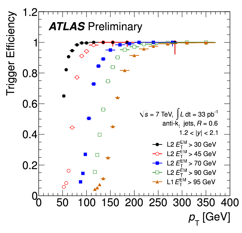
The MBTS trigger is used to select jets between 20 GeV and 60 GeV, whereas central and forward jet triggers are used to select jets with GeV. In the first runs (Period 1), the jet trigger was using only the L1 decision to reject events, whereas starting from September (Period 2) the L2 decision was also used for rejection. The threshold in the L2 is typically 15 GeV larger than the L1 threshold in the same trigger chain, except for the L1 10 GeV threshold that corresponds to the L2 15 GeV threshold. As explained in Section 2.7, the trigger thresholds are at the EM scale. Figure 3.6 shows the trigger efficiency as a function of the trigger threshold and the calibrated jet in four representative regions.
Given the increase of the instantaneous luminosity during 2010, prescales have been applied to jet triggers with low thresholds in order to control the trigger rate. For each jet and rapidity bin in this analysis, a trigger is used to select jets such that is fully efficient () and that the prescale is as low as possible. The trigger efficiency for a given energy threshold, , is computed with a sample of the events passing a trigger with a lower threshold, . The efficiency is defined as the fraction of jets passing the trigger with threshold with respect to the number of jets passing the trigger with threshold.
Tables 3.1 and 3.2 show the trigger used in each jet and bin. In the region , the central jet trigger (L1_J, L2_J) is used. The trigger has lower efficiency in than in the rest of the central region. This is due to the fact that between of 1.3 and 1.5, there is a transition between the barrel and the end-cap of the liquid argon calorimeter. The electronic signals from these two parts of the calorimeter are not added up at the trigger level to integrate over the full jet energy deposition. The logical OR of central and forward (L1_JF, L2_JF) jet triggers is used in the rapidity range , since none of them are fully efficient alone. The forward jet trigger is used in the bin .



| Period 1 | Period 1 | Period 2 | Period 2 | |
|---|---|---|---|---|
| (GeV) | ||||
| 60-80 | L1_J5 | L1_J5 | L2_J15 | L2_J15 |
| 80-110 | L1_J15 | L1_J5 | L2_J30 | L2_J15 |
| 110-160 | L1_J30 | L1_J15 | L2_J45 | L2_J30 |
| 160-210 | L1_J55 | L1_J30 | L2_J70 | L2_J45 |
| 210-260 | L1_J75 | L1_J55 | L2_J90 | L2_J70 |
| 260-310 | L1_J95 | L1_J75 | L1_J95 | L2_J90 |
| 310-400 | L1_J115 | L1_J95 | L1_J115 | L1_J95 |
| L1_J115 | L1_J115 | L1_J115 | L1_J115 |
| Period 1 | Period 1 | Period 2 | Period 2 | |
|---|---|---|---|---|
| (GeV) | ||||
| 60-80 | L1_J10 L1_FJ10 | L1_J10 | not used | L2_FJ25 |
| 80-110 | L1_J10 L1_FJ10 | L1_J30 | L2_J25 L2_FJ25 | L2_FJ25 |
| 110-160 | L1_J30 L1_FJ30 | L1_J55 | L2_J45 L2_FJ45 | L2_FJ45 |
| 160-210 | L1_J55 L1_FJ55 | L1_J55 | L2_J45 L2_FJ45 | L2_FJ70 |
| L1_J55 L1_FJ55 | L1_J55 | L2_J70 L2_FJ70 | L2_FJ70 |
3.4 Unfolding to the particle level
The measured differential cross section with respect to the jet and is defined as follows:
| (3.2) |
where is the number of jets in the and bins, and is the integrated luminosity.
This cross section is corrected for detector effects back to the particle level with a bin-by-bin unfolding procedure, using PYTHIA 6.423 with the AMBT1 tune simulated samples. In order to improve the agreement between the MC and the data, the MC is reweighted in order to scale its prediction, that uses a modified LO PDF, to that of a NLO PDF. Corrections are derived in each and bin by computing the ratio between the inclusive jet distributions using truth jets (including muons and neutrinos) and using calorimeter simulated jets. These corrections are multiplied to equation 3.2, and have values between 0.8 and 1.0 in most jet regions, and around 0.6 at very low and very high jet .
3.5 Systematic Uncertainties
In this section several sources of systematic uncertainty on the measurement are considered. More emphasis is given to the explanation of the JES uncertainty, since it is the main contribution to the total uncertainty on the inclusive jet cross section measurement.
3.5.1 JES uncertainty
The JES uncertainty comes mainly from the uncertainty on the single particle response, limitations in the detector knowledge (such as the amount of dead material), and the physics models and parameters (mainly fragmentation and underlying event) in the MC event generator used to derive the JES corrections. Seven bins have been selected to estimate the JES uncertainty, taking into account the position of the different calorimeters (see Figure 3.2). The JES uncertainty is first calculated in the region and then propagated forward in rapidity using a jet balance technique, explained later in this section. The reason is that the detector is better known in the central region, and that test-beam measurements to estimate the uncertainty due to the calorimeter response to single particles were only performed in the range .
Uncertainty on the calorimeter response to single particles
The calorimeter response to single hadrons has been studied comparing the calorimeter energy response to the momentum of isolated tracks [51]. Results have been obtained from pp collisions at 0.9 and 7 TeV, finding an agreement between data and MC within 2-5% for tracks with momentum between 0.5 to 20 GeV. The calorimeter response to particles with momentum in the range between 20 GeV and 350 GeV has been derived from test-beam measurements, in which pion beams with momentum up to 350 GeV were injected into a slice of the ATLAS detector. For particles with larger momentum, an additional uncertainty of 10% on top of the 350 GeV measured uncertainty is applied in order to take into account longitudinal leakage and calorimeter non-linearities. The uncertainty of the single particle response in the calorimeter has been used to derive the related jet energy scale uncertainty. This is done using MC, and varying randomly the energy of the particles of the jets separately, and according to the values of the single particle response uncertainty. The JES calibration constants are then computed with these modified jets and the results are compared to the nominal constants in order to derive the uncertainty. The uncertainty on the jet increases from to with increasing jet .
Uncertainties due to the detector simulation
Since the JES calibration is derived using MC samples, deviations in the description of the detector in the MC introduce an uncertainty on the JES. This has been estimated by varying the material budget in the simulation. In the particle range of the E/p studies using isolated tracks only the dead material in the inner detector has been varied, since the measurement is already performed with the ATLAS detector. For other particles, also changes in the calorimeter material have been simulated. The jet response in these modified samples is compared to the nominal one in order to estimate the systematic uncertainty, that is always below .
As explained in Section 2.4.3, clusters are build by adding neighboring cells with signal over noise above certain thresholds. Therefore, miss-modeling of the calorimeter cell noise in the MC would lead to different cluster formation that eventually would affect the jet reconstruction. The impact of possible miss-modeling of the noise has been evaluated by varying the signal over noise thresholds in the cluster reconstruction. The difference of the jet energy response for jets reconstructed with the modified noise thresholds and the nominal jets has been taken as a systematic uncertainty. This goes up to for jets with GeV, and is negligible at higher .
Uncertainties due to the event modelling in the Monte Carlo generators
The jet energy response obtained using PYTHIA with the AMBT1 tune, used to derive the corrections, has been compared with those obtained using ALPGEN+HERWIG+JIMMY and PYTHIA with the Perugia2010 tune. This estimates the uncertainty due to the different QCD description contained in the MCs, such as fragmentation or underlying event. It goes from at low to for GeV.
Uncertainties due to the relative calibration in the forward regions
As already mentioned, the JES uncertainties are evaluated for jets with . These uncertainties are transferred to the forward region by using a balance technique in which the of forward jets is measured relative to that of central jets in dijet events. The difference of the balance of a central and a forward jet in data and in MC is taken as a systematic uncertainty, that is added in quadrature to the JES uncertainty in the central region. This is the largest source of uncertainty at low in the forward region, going up to around 12%. For jets with GeV it is always smaller than 2%.
Uncertainty of the method to derive the JES calibration constants
There is an uncertainty associated to the method used to derive the JES calibration constants. It comes mainly from the assumption that every jet needs the same average compensation and from the fact that the same correction factor is used for the energy and the , whereas the jet mass is not always zero. Two statistical independent MC samples were used to derive the uncertainty associated to the method itself. One was used to derive the corrections, that were applied to the calorimeter jets of the other. Deviations of the jet response from unity in this second sample are taken as systematic uncertainties, that are generally below , apart from the central region, where the uncertainty amounts up to at low .
Total uncertainty on the jet
In Figure 3.7, the fractional JES uncertainty and its components are shown as a function of in three representative regions. The fractional JES uncertainty is below for GeV in all regions, it is smaller than for all in the central region, and amounts up to at low in the most forward region.
Uncertainty due to multiple interactions
A final contribution to account for the uncertainty due to pile-up is added in quadrature in events with more than one primary vertex. This uncertainty is estimated mainly from the variation of the offset corrections derived using tracks instead of calorimeter towers. It is shown in Figure 3.8 for events with two primary vertices. In this case, the uncertainty due to pile-up for low jets is around 1% in the central region and almost 2.5% in the most forward region. The uncertainty is always below 1% for jets with GeV. In the case of three primary vertices, the pile-up uncertainty is approximately twice that of two primary vertices, and with four primary vertices the uncertainty for central, endcap and forward jets is less than 3%, 6% and 8%, respectively. The relative uncertainty due to pile-up for events with 5 additional interactions becomes less than 1% for all jets with GeV.
Uncertainty on the measurement due to the JES uncertainty
The JES uncertainty is the largest contribution to the uncertainty of the inclusive jet cross section measurement, that goes from around +30%/-20% in the central region to approximately +80%/-50% in the most forward region.


3.5.2 Other sources of systematic uncertainties
- •
The unfolding factors have been recomputed varying the jet in the MC in order to take into account the jet energy and angular resolution, and the differences on the cross section shape in data and in MC. These unfolding factors have been compared to estimate the systematic uncertainty, that is typically between and , except for the lowest bin where it goes up to 20%.
- •
Matching of track jets to calorimeter jets has been performed in both data and Monte Carlo to estimate the modeling of the calorimeter jet reconstruction efficiency in the MC. The difference is smaller than 2% (3%) for jets with GeV (30 GeV), and is taken as a systematic uncertainty.
- •
In this analysis, jets are selected with triggers that are 99% efficient. A conservative 1% uncertainty overall has been considered to account for the trigger inefficiency.
- •
The systematic uncertainty on the efficiency of the jet quality criteria is taken as a systematic uncertainty on the cross section, and it is always below 1%.
- •
Finally, the uncertainty on the luminosity measurement is 3%.
3.6 Results
The inclusive jet cross section unfolded to the hadron level is shown in Figure 3.9 for different regions up to . It is measured from 20 GeV to 1.5 TeV and spans up to ten orders of magnitude. The data are compared to NLO predictions corrected for non-perturbative effects. The NLO predictions are obtained from NLOJET++4.1.2 program with CTEQ 6.6 PDFs, and the corrections for non-perturbative effects are derived using samples produced with PYTHIA 6.423 with the AMBT1 tune and applied to NLO predictions. These corrections are obtained bin-by-bin, comparing the cross section with and without hadronization and underlying event. The correction is dominated by the underlying event at low (1.5 at 20 GeV), and tends to 1 as the increases. The uncertainty on the NLO predictions is obtained adding in quadrature uncertainties from the PDFs, the choice of factorization and renormalization scales, and the value of the strong coupling constant. It is combined with the uncertainty on the non-perturbative corrections, estimated from the maximum difference of the corrections with AMBT1 with respect to other PYTHIA tunes and to HERWIG++. The total uncertainty in the predictions is typically around 20% at low and high and 10% at intermediate values.
Figure 3.10 shows the ratio of the measured cross section in data and the theory prediction, that are in agreement within uncertainties. The cross section in data is lower than the cross section predicted by NLO predictions in the forward region and at high .
In Figure 3.11, data are compared to results using CTEQ 6.6, MTSW 2008, NNPDF 2.1, and HERAPDF 1.5. All cross sections are normalized to that obtained with CTEQ 6.6. Predictions using MTSW 2008, NNPDF 2.1, and HERAPDF 1.5 are closer to data than those using CTEQ 6.6, but all have the tendency to produce higher cross sections than data at high in the forward region. This may be due to the fact that PDFs are currently poorly constrained in this kinematic region.
Finally, Figure 3.12 shows the comparison of data and POWHEG predictions using MTSW 2008, both normalized to the NLO with MTSW 2008 cross section shown in Figure 3.11. POWHEG is interfaced with either PYTHIA or HERWIG for the parton showering, the hadronization and the underlying event modeling. POWHEG predictions agree with data within uncertainties, but tend to produce larger cross section at low and, mainly POWHEG+HERWIG, smaller cross sections at high . POWHEG gives different results depending on whether PYTHIA or HERWIG is used for the showering, which may be taken as an indication of the level of uncertainty related to the parton shower implementation.


Chapter 4 Jet Shapes
One of the fundamental elements of jet measurements is the proper understanding of the energy flow around the jet core and the validation of the QCD description contained in the event generators, such as parton shower cascades, and the fragmentation and underlying event models. Jet shapes [52] observables are sensitive to these phenomena and thus very adequate to this purpose. They have been measured in [53], [54], and [55] colliders.
Before the first pp collisions delivered by the LHC, the sensitivity of jet shapes to the UE and pile-up in ATLAS was shown using MC simulation at 10 TeV [56] (see Appendix A). Jet shapes studies at detector level were performed with the very first ATLAS data at a center of mass energy of 900 GeV [57], [58] (see Appendix B).
Results at calorimeter level using 7 TeV data were used in the first measurement of the inclusive jet cross section in ATLAS [40] based on 17 nb-1 to validate the QCD description in the event generators and to consolidate the confidence in the corrections and calibrations applied. Jet shapes at calorimeter level in the forward region () have been computed with the same purpose for the inclusive jet cross section measurement using the full 2010 dataset [41], corresponding to 37 pb-1.
In this Chapter, measurements of differential and integrated jet shapes in proton-proton collisions at TeV are presented [59], using data collected by the ATLAS experiment corresponding to pb-1 of total integrated luminosity. The definition of jet shapes observables and the event selection criteria are explained, followed by a description of Monte Carlo samples used and a detailed discussion on the corrections for detector effects and systematic uncertainties. Finally, results are presented and compared to predictions from several MC event generators.
4.1 Jet shape definition
The differential jet shape as a function of the distance to the jet axis is defined as the average fraction of the jet that lies inside an annulus of inner radius and outer radius around the jet axis:
| (4.1) |
where denotes the scalar sum of the of the jet constituents in the annulus between radius and , is the number of jets, and and are used. The points from the differential jet shape at different values are correlated since, by definition, . Alternatively, the integrated jet shape is defined as the average fraction of the jet that lies inside a cone of radius concentric with the jet cone:
| (4.2) |
where, by definition, , and the points at different values are strongly correlated. This geometrical definition of the shape of the jet, based on concentric cones around the jet axis, is particularly adequate for jets reconstructed using the anti- algorithm.
In this analysis, the jet finding algorithm is run over uncorrected energy clusters or towers (calorimeter level), Inner Detector tracks, or final-state particles in the MC generated events (particle level). The jet shape measurements are performed in different regions of jet and , and a minimum of 100 jets in data are required in each region to limit the statistical fluctuations on the measured values.
4.2 Event selection
The event and jet selection criteria, close to that of the inclusive jet cross section measurement detailed in Section 3.3, are:
- •
Detector components relevant for this analysis, such as the calorimeter and the Inner Detector, operating at the nominal conditions.
- •
Only data from runs until the end of August are used, in order to avoid bunch train pile-up 11 1 Bunch train pile-up refers to the energy deposit coming from pp collisions in a different bunch crossing than the one of the event under consideration.. This corresponds to pb-1 of total integrated luminosity collected by the ATLAS experiment.
- •
The trigger is required to be fully efficient in each and bin.
- •
The events are required to have one and only one reconstructed primary vertex with a -position within 10 cm of the origin of the coordinate system, which suppresses pile-up contributions from multiple proton-proton interactions in the same bunch crossing, beam-related backgrounds and cosmic rays. The tight cut on the -position is performed in order to keep the projective geometry of the calorimeter.
- •
Only jets with corrected transverse momentum GeV and rapidity are considered.
4.3 Monte Carlo simulation
Monte Carlo simulated samples are used to correct the jet shapes for detector effects back to the hadron level, and to estimate part of the systematic uncertainties. PYTHIA 6.4.21, HERWIG++ 2.4.2 and ALPGEN 2.13 event generators are used to produce inclusive jet events in proton-proton collisions at TeV. In the case of PYTHIA, samples are generated using three tuned sets of parameters denoted as ATLAS-MC09, DW, and Perugia2010. In addition, a special PYTHIA-Perugia2010 sample without UE contributions is generated using the RIVET package [60]. HERWIG++ and PYTHIA-MC09 samples are generated with MRST2007LO∗ [11] [21] PDFs, PYTHIA-Perugia2010 and PYTHIA-DW with CTEQ5L [61] PDFs, and ALPGEN with CTEQ61L [62] PDFs.
4.4 Jet shapes at calorimeter level
The measured differential (integrated) jet shapes, as determined by using calorimeter clusters, are shown in Figures 4.1 and 4.2 (Figures 4.3 and 4.4). The data present a prominent peak at low , which indicates that the majority of the jet momentum is concentrated around the jet axis. As expected, jets get narrower as the increases. The data are compared to several MC predictions, being PYTHIA-Perugia2010 the one that describes the data best. A reasonable agreement between jet shapes data and PYTHIA-Perugia2010 has been also observed in the different regions considered in this analysis. Therefore, PYTHIA-Perugia2010 is used to correct both differential and integrated jet shapes for detector effects back to the particle level.


4.5 Correction for detector effects
The correction for detector effects is done using a bin-by-bin procedure that also accounts for the efficiency of the selection criteria and of the jet reconstruction in the calorimeter. Here, the method is described in detail for the differential case. A similar procedure is employed to correct independently the integrated measurements. The correction factors are computed separately in each jet and region. They are defined as the ratio between the jet shapes at the particle level , obtained using particle-level jets in the kinematic range under consideration, and the reconstructed jet shapes at the calorimeter level , after the selection criteria are applied and using calorimeter-level jets in the given and range.
The correction factors present a moderate and dependence and vary between 0.95 and 1.1 as increases. For the integrated jet shapes, the correction factors differ from unity by less than . This is shown in Figures 4.5 and 4.6 (4.7 and 4.8) for the differential (integrated) jet shapes. The corrected jet shape measurements in each and region are computed by multiplying bin-by-bin the measured uncorrected jet shapes in data by the corresponding correction factors.


4.6 Systematic uncertainties
A detailed study of systematic uncertainties on the measured differential and integrated jet shapes has been performed. The impact on the differential measurements is described here.
- •
The absolute energy scale of the individual clusters belonging to the jet is varied in the data according to studies using isolated tracks [40], which parametrize the uncertainty on the calorimeter cluster energy as a function of and of the cluster. This variation is performed by multiplying the cluster energies by for up (down) variation, with a = 5% if (a = 10% if ), b = 1.5, and in GeV. The jet position is then recalculated according to the new cluster four-momenta. The maximum variation on the differential jet shapes is taken as a systematic uncertainty, that varies typically between 3 to 15 as increases, and constitutes the dominant systematic uncertainty in this analysis (see Figures 4.9 and 4.10).
- •
The systematic uncertainty on the measured jet shapes arising from the details of the model used to simulate calorimeter showers in the MC events is studied. A different simulated sample is considered, where the FRITIOF [63] plus BERT showering model is employed instead of the QGSP plus BERT model. FRITOF+BERT provides the second best description of the test-beam results [46] after QGSP+BERT. This introduces an uncertainty on the measured differential jet shapes that varies between to 4, and is approximately independent of and (see Figures 4.11 and 4.12).
- •
The measured jet is varied by 2 to 8, depending on and , to account for the remaining uncertainty on the absolute jet energy scale [40], after removing contributions already accounted for and related to the energy of the single clusters and the calorimeter shower modeling, as discussed above. This introduces an uncertainty of about 3 to 5 in the measured differential jet shapes (see Figures 4.9 and 4.10).
- •
- •
The correction factors are recomputed using HERWIG++, which implements different parton shower, fragmentation and UE models than PYTHIA, and compared to PYTHIA-Perugia2010 (see Figures 4.15 and 4.16). In addition, the correction factors are also computed using ALPGEN and PYTHIA-DW for GeV, where these MC samples provide a reasonable description of the uncorrected shapes in the data. The results from HERWIG++ encompass the variations obtained using all the above generators and are conservatively adopted in all and ranges to compute systematic uncertainties on the differential jet shapes. These uncertainties increase between 2 and 10 with increasing r.
- •
Two statistically independent samples are used to test the closure of the correction for detector effects procedure. One was used to compute the shapes using calorimeter clusters, while the other was used to correct these shapes for detector effects. In Figures 4.17 and 4.18 corrected results from the first sample are compared to results at particle level from the second one. The ratio between the two deviates from unity about 1, value that is included as uncertainty on the differential measurements.
- •
No significant dependence on instantaneous luminosity is observed in the measured jet shapes, indicating that residual pile-up contributions are negligible after selecting events with only one reconstructed primary vertex.
- •
It was verified that the presence of dead calorimeter regions in the data does not affect the measured jet shapes, since only affected a small fraction of jets.
The different systematic uncertainties are added in quadrature to the statistical uncertainty to obtain the final result. The total systematic uncertainty for differential jet shapes decreases with increasing and varies typically between 3 and 10 (10 and 20) at () (see Figures 4.19 and 4.20). The total uncertainty is dominated by the systematic component, except at very large where the measurements are still statistically limited. In the case of the integrated measurements, the total systematic uncertainty varies between 10 and ( and ) at () as increases, and vanishes as approaches the edge of the jet cone (see Figures 4.21 and 4.22).


4.6.1 Cross-checks using other detector objects
The jet shape analysis is also performed using tracks inside the cone of jets reconstructed using calorimeter clusters. The inner detector tracks are required to pass selection criteria derived in the analysis of charged particle multiplicities in ATLAS [64]:
- •
MeV and
- •
a hit in the first layer (layer-0) of the Pixel detector if one is expected (meaning that the layer-0 module is not out of the configuration and the track is not close to the module edge)
- •
a minimum of one Pixel hit in any of the 3 layers of this detector
- •
at least two (if MeV), four(if MeV) or six (if MeV) SCT hits
- •
transverse and longitudinal impact parameters calculated with respect to the event primary vertex mm and mm respectively
- •
probability for reconstructed tracks with GeV, to remove high miss-measured tracks
This provides an alternative method to measure the internal structure of jets based on charged particles. The measurements are limited to jets with , as dictated by the tracking coverage and the chosen size of the jet. Figures 4.23 and 4.24 show the differential jet shapes in this rapidity range using tracks and clusters respectively. The ratio of the jet shapes using clusters and tracks in data are compared to that in the Monte Carlos simulation (Figure 4.25). Maximum deviations from one of these ratios are about 5, well within the quoted systematic uncertainties.
Finally, the jet shapes results are obtained using calorimeter towers of fixed size ( space) instead of topological clusters as input to the jet reconstruction algorithm. In order to suppress noise, the towers are built only with cells that belong to a cluster. Figure 4.26 show that tower jets are significantly broader than cluster jets before correcting for detector effects. Instead, differences reduce to less than 5 after applying the corrections, as shown in Figure 4.27. Again, the observed differences are well inside the quoted uncertainty on the nominal results based on calorimeter clusters.


4.7 Results
The measurements presented in this Chapter refer to differential and integrated jet shapes, and , corrected at the particle level and obtained for anti- jets with distance parameter in the region and . The measurements are presented in separate bins of and . Tabulated values of the results are available in Ref. [65].
Figures 4.28 to 4.30 (4.31 to 4.33) show the measured differential (integrated) jet shapes as a function of in different ranges. The dominant peak at small indicates that the majority of the jet momentum is concentrated close to the jet axis. At low , more than 80 of the transverse momentum is contained within a cone of radius around the jet direction. This fraction increases up to 95 at very high , showing that jets become narrower as increases. This is also observed in Figure 4.34, where the measured , the fraction of the jet transverse momentum outside a fixed radius , decreases as a function of .
The data are compared to predictions from HERWIG++, ALPGEN, PYTHIA-Perugia2010, and PYTHIA-MC09 in Figure 4.28 to Fig. 4.34(a); and to predictions from PYTHIA-DW and PYTHIA-Perugia2010 with and without UE contributions in Figure 4.34(b). The jet shapes predicted by PYTHIA-Perugia2010 provide a reasonable description of the data, while HERWIG++ predicts broader jets than the data at low and very high . The PYTHIA-DW predictions are in between PYTHIA-Perugia2010 and HERWIG++ at low and produce jets which are slightly narrower at high . ALPGEN is similar to PYTHIA-Perugia2010 at low , but produces jets significantly narrower than the data at high . PYTHIA-MC09 tends to produce narrower jets than the data in the whole kinematic range under study. The latter may be attributed to an inadequate modeling of the soft gluon radiation and UE contributions in PYTHIA-MC09 samples, in agreement with previous observations of the particle flow activity in the final state [66]. Finally, Figure 4.34(b) shows that PYTHIA-Perugia2010 without UE contributions predicts jets much narrower than the data at low . This confirms the sensitivity of jet shape observables in the region GeV to a proper description of the UE activity in the final state 22 2 These conclusions are supported by energy flow results at detector level, reported in Appendix C..
The dependence on is shown in Figure 4.35 and 4.36, where the measured jet shapes are presented separately in five different jet rapidity regions and different bins, for jets with GeV. At high , the measured shape presents a mild dependence, indicating that the jets become slightly narrower in the forward regions. This tendency is observed also in the various MC samples. Similarly, Figures 4.37 and 4.38 present the measured as a function of in the different regions compared to PYTHIA-Perugia2010 predictions.
Finally, and only for illustration, the typical shapes of quark- and gluon-initiated jets, as determined using events generated with PYTHIA-Perugia2010, are also shown in Figures 4.37 and 4.38. For this purpose, MC events are selected with at least two particle-level jets with GeV and in the final state. The two leading jets in this dijet sample are classified as quark-initiated or gluon-initiated jets by matching (in space) their direction with one of the outgoing partons from the QCD hard process. At low the measured jet shapes are similar to those from gluon-initiated jets, as expected from the dominance of hard processes with gluons in the final state. At high , where the impact of the UE contributions becomes smaller (see Figure 4.34(b)), the observed trend with in the data is mainly attributed to a changing quark- and gluon-jet mixture in the final state, convoluted with perturbative QCD effects related to the running of the strong coupling.
The jet shapes results presented in this Chapter were obtained with the first collisions at TeV, in which the pile-up can be neglected, and were published in [59]. They indicate the potential of jet shape measurements at the LHC to constrain the phenomenological models for soft gluon radiation, underlying event (UE) activity, and non-perturbative fragmentation processes in the final state. After the publication of these results, additional comparisons to predictions from different MC programs have been performed [67]. They are reported in the next Chapter, which includes tests to the data points for all the MC models considered.


Chapter 5 Jet Shapes in ATLAS and Monte Carlo modeling
In this Chapter the jet shapes results published in [59] are compared to predictions of different MC programs, that include recent tuned sets of parameters to describe the ATLAS minimum bias (MB) and jet data.
5.1 Monte Carlo samples
The MC generators considered in this Chapter are listed below.
- •
The PYTHIA 6.4.23 generator is used to produce QCD-jet inclusive samples with both AMBT1 and AUET2 [68] tunes, as determined by ATLAS, and with the Perugia2011 tune [20]. PYTHIA-AMBT1 is based on MRST LO* parton density functions (PDFs) inside the proton, and uses as input results from the ATLAS charged particle MB analysis at TeV and TeV. PYTHIA-AUET2 is based on MRST LO** PDFs, uses also as input ATLAS UE data [69], and includes a modified final-state parton shower from initial-state radiated partons to describe the CDF [53] and ATLAS jet shape measurements. The PYTHIA-Perugia2011 tune uses CTEQ5L PDFs and constitutes an updated version of the PYTHIA-Perugia2010 tune, as inspired by the comparison with early LHC data. Samples are also generated using the PYTHIA 8.145 program [70] which, among other updates, includes a fully interleaved -ordered evolution for initial- and final-state gluon radiation and multiple parton interactions (MPI). The Pythia 8 samples are produced with the 4C tune [70] for the UE modeling, based on CTEQ6L1 PDFs and using Tevatron and ATLAS data as input.
- •
QCD-jet inclusive samples are generated with the Herwig++ 2.4.2 and Herwig++ 2.5.1 programs. The Herwig++ 2.4.2 predictions used in [59] suffered from a wrong setting in the ATLAS generation of the MC samples, related to the parameters that control the contribution from MPI, which a priori would affect the comparison with the data at low . In this Chapter, the same Herwig++ 2.4.2 predictions already presented in the previous Chapter (here denoted as Herwig++ 2.4.2 bug), are compared with correctly generated HERWIG 2.4.2 predictions. Herwig++ 2.5.1 includes a modified algorithm for color reconnection between clusters before hadronization and new color connections between soft scatters and the beam remnants that improve the description of the MB data and UE-related observables at the LHC. In the case of Herwig++ 2.4.2 the LO∗ tune [71] is employed, while the UE7 tune [72] is used for Herwig++2.5.1 predictions. In addition, samples are produced with HERWIG 6.510 interfaced with JIMMY 4.31 to model the UE contributions with both AUET1-LO∗ [73] and AUET2-LO∗∗ [68] tunes, as determined by ATLAS using data at 0.9 TeV and 7 TeV.
- •
QCD-jet events are generated using the ALPGEN 2.13 program interfaced with PYTHIA 6.423 for the parton shower and fragmentation into hadrons. The samples are produced with CTEQ6L1 PDFs and the Perugia6 tune to model the UE contributions.
- •
The Sherpa 1.2.3 and Sherpa 1.3.0 programs [74] are used to generate QCD-jet samples. Default settings include CTEQ66 PDFs and MPI tuned to Tevatron and ATLAS data. The Sherpa 1.3.0 version contains a modified parton shower evolution via pre-factors within , as motivated by next-to-leading-logarithm (NLL) perturbative QCD (pQCD) calculations, that improve the description of the measured Z boson in ATLAS. Samples with different matrix element multiplicities are produced, with the aim to illustrate the impact of higher-order contributions to the description of the jet shapes. Samples with only hard processes and with up to partons in the final state are considered, and interfaced with parton showers.
- •
QCD-jet samples are generated with the POWHEG-BOX r302 program, which includes next-to-leading order (NLO) pQCD predictions for inclusive jet production, interfaced either with PYTHIA 6.423 or with HERWIG 6.510 plus JIMMY 4.31 for parton shower, fragmentation into hadrons, and to model the underlying event. For the latter, the AMBT1 or AUET1-LO∗ tunes are used, respectively.
The simulated event samples were produced using the ATLAS interface to the generators and the Rivet system was used to analyze the samples and produce the relevant jet shape observables.
5.2 Results
Different observables in data are compared to the MC predictions. This includes the measured differential jet shape for jets with in eight bins within the range GeV, and the integrated jet shape as a function of in different regions and as a function of in different bins.
5.2.1 Comparison with PYTHIA
The measured jet shapes are compared to the different PYTHIA predictions in Figures 5.1 to 5.5. As expected, PYTHIA6-AMBT1 tends to produce jets slightly narrower than the data as it underestimates the UE activity in dijet events [68] and lacks a tuned final-state parton shower from the initial-state radiation. PYTHIA6-AUET2, PYTHIA6-Perugia2011, and Pythia 8-4C provide a good description of the measured jet shapes in the whole jet kinematic range considered 11 1 The reader should note that the ATLAS jet shapes measurements are input to the PYTHIA6-AUET2 tune..
5.2.2 Comparison with Herwig++ and HERWIG/JIMMY
The measurements are compared to the predictions from Herwig++ 2.4.2, Herwig++ 2.5.1, and HERWIG/JIMMY programs in Figure 5.6 to Figure 5.10. As shown in the Figures, the effect of the wrong setting in Herwig++ 2.4.2 bug (see Section 2) is only visible for jets with GeV. Herwig++ 2.4.2 provides a reasonable description of the data in the whole jet kinematic range considered. HERWIG/JIMMY, which includes the AUET2 tune, describes the data best. Finally, Herwig++ 2.5.1 tends to produce jets narrower than the data.
5.2.3 Comparison with ALPGEN and Sherpa
The data are compared to the predictions from Sherpa 1.2.3 ( process), Sherpa 1.2.3 (up to process), Sherpa 1.3.0 ( process), and ALPGEN interfaced with PYTHIA in Figure 5.11 to Figure 5.15. Comparisons with ALPGEN interfaced with HERWIG and JIMMY were presented in [59]. The different Sherpa predictions are similar and provide a reasonable description of the data. This indicates that the presence of additional partons from higher-order matrix elements contributions do not affect the predicted jet shapes, mainly dictated by the soft radiation in the parton shower. The comparison between Sherpa 1.2.3 and Sherpa 1.3.0 shows that the NLL-inspired corrections included in the latter for the parton shower do not impact significantly the predicted jet shapes. ALPGEN interfaced with PYTHIA predicts too-narrow jets and does not describe the data. This was already the case for ALPGEN interfaced with HERWIG and JIMMY [59] and requires further investigation to determine whether the disagreement observed with the data can be completely attributed to the UE modeling in the MC samples or it is also related to the prescription followed by ALPGEN in merging the partons from the matrix elements with the parton showers in the final state.
5.2.4 Comparison with POWHEG
The impact of the presence of higher-order matrix elements contributions on the predicted jet shapes is further studied in Figure 5.16 to Figure 5.20, where the data are compared to the predictions from POWHEG interfaced with PYTHIA or HERWIG/JIMMY, as well as to standalone PYTHIA and HERWIG/JIMMY predictions. For these comparisons, AMBT1 and AUET1-LO∗ tuned sets of parameters are used for PYTHIA and HERWIG/JIMMY, respectively. In general, the jet shapes predicted by POWHEG follow the trend of the corresponding standalone predictions. POWHEG interfaced with HERWIG/JIMMY provides a reasonable description of the data while the interface with PYTHIA predicts too-narrow jets. This confirms that the shape of the jet is mainly dictated by the parton shower implementation and the details of the UE modeling in the final state.


5.2.5 statistical tests
Finally, a test is performed to the data points in Figures 4.38, 5.5, 5.10, 5.15, and 5.20 with respect to a given MC prediction, separately in each rapidity region. The systematic uncertainties are considered independent and fully correlated across bins, and the test is carried out according to the formula
| (5.1) |
where is the measured data point in bin , is the corresponding MC prediction, and denotes the vector of standard deviations, , for the different independent sources of systematic uncertainty. For each rapidity region considered, the sums above run over the total number of data points in and five independent sources of systematic uncertainty, and the is minimized with respect to . Correlations among systematic uncertainties are taken into account in .
The results for the different MC predictions shown in this and in the previous Chapter are collected in Table 5.1.
| range | |||||
| degrees of freedom (d.o.f) | 10 | 10 | 10 | 10 | 8 |
| PYTHIA-Perugia2010 | 0.6 | 1.8 | 2.4 | 1.4 | 1.4 |
| HERWIG++ | 2.2 | 2.3 | 3.1 | 1.8 | 4.0 |
| PYTHIA-MC09 | 1.0 | 2.5 | 2.4 | 1.5 | 3.2 |
| PYTHIA-DW | 2.4 | 3.4 | 6.9 | 4.0 | 5.2 |
| ALPGEN | 3.8 | 9.8 | 7.4 | 6.7 | 6.0 |
| PYTHIA-Perugia2010 (no UE) | 4.2 | 9.7 | 4.9 | 8.6 | 4.8 |
| PYTHIA6-AMBT1 | 1.6 | 2.9 | 4.4 | 2.4 | 4.4 |
| PYTHIA6-AUET2 | 0.8 | 2.1 | 2.3 | 1.3 | 3.3 |
| PYTHIA6-Perugia2011 | 0.5 | 2.2 | 1.7 | 1.3 | 1.6 |
| Pythia 8-4C | 1.3 | 3.6 | 1.6 | 1.6 | 2.7 |
| Herwig++ 2.4.2 | 0.9 | 2.7 | 2.9 | 2.4 | 2.9 |
| Herwig++ 2.5.1 | 4.2 | 10.9 | 1.0 | 8.6 | 1.7 |
| HERWIG/JIMMY-AUET2 | 3.6 | 3.6 | 5.3 | 3.4 | 6.4 |
| HERWIG/JIMMY-AUET1 | 3.8 | 4.1 | 4.0 | 2.9 | 2.7 |
| Sherpa 1.2.3 (up to ) | 1.3 | 1.2 | 0.9 | 1.2 | 1.1 |
| Sherpa 1.2.3 () | 1.8 | 5.3 | 0.7 | 3.0 | 4.0 |
| Sherpa 1.3.0 () | 3.0 | 8.1 | 1.1 | 5.7 | 1.7 |
| ALPGEN+PYTHIA | 4.9 | 14.9 | 10.6 | 8.6 | 6.7 |
| POWHEG+PYTHIA | 1.9 | 3.6 | 4.4 | 1.7 | 1.1 |
| POWHEG+HERWIG | 4.7 | 9.8 | 9.4 | 2.2 | 2.4 |
Conclusions
This Thesis describes the measurements of the inclusive jet cross section and jet shapes in
collisions at TeV using the ATLAS detector. The anti- algorithm with
is used to reconstruct jets. Both measurements are unfolded back to the hadron level and compared to
theory predictions.
The inclusive jet cross section measurement has been performed using jets with GeV
and in a data sample corresponding to a total luminosity of pb-1 collected by ATLAS during 2010.
The measurement constitute a stringent test of pQCD over ten orders of magnitude,
covering a jet range up to 1.5 TeV.
The measurement expands by a factor of the kinematic region in probed by the Tevatron,
in a wider range.
The data are compared with NLO predictions using several PDFs corrected for non-perturbative effects.
A general agreement is found, but the predicted cross section tends to be larger than that in data
at high in the forward region. This can be atributted to the current PDF of the gluon at high ,
showing the potential of the measurement to constrain the parton distribution functions when used in global fits.
The measurement of jet shapes in inclusive jet production uses 3 pb-1 collected by ATLAS,
for jets with GeV and . It is important to notice that the measurement was
performed with the very first collisions at 7 TeV center-of-mass-energy, when the LHC luminosity
was low enough to collect a data sample clean of pile-up.
The jet shape measurements can be used to constrain the phenomenological models for soft gluon radiation, underlying event (UE)
activity, and non-perturbative fragmentation processes in the final state.
This is particularly important for searches of new physics that require a good control of the soft physics.
The jet shape measurements constitute a first step towards the study of boosted topologies corresponding to the
decay of heavy particles, that promise to play a central role in the serach for a light Higgs boson or in
searches for new physics.
The integrated luminosity recorded by ATLAS has already increased above during 2011. The inclusive
jet cross section is being updated with these new data, and further studies are being done in order to reduce the JES uncertainty.
The large dataset being recorded will also allow to perform sensitive jet substructure analyses
searching for new physics.
Appendix A Sensitivity of the jet shapes to the underlying event and to the pile-up using MC simulated events
Before the first collisions were delivered by the LHC, studies on jet shapes were performed using PYTHIA QCD-dijet Monte Carlo simulated events in collisions at TeV. The effect of the underlying event and the pileup on the jet shapes was investigated in jets reconstructed with the SISCone algorithm with R = 0.7 and splitting-merging fraction equal to 0.75.
Figures A.1, A.2 and A.3 show the comparison of jet shapes at hadron level in events with and without underlying event. As expected, the presence of the underlying event translates into broader jets at low . The jet shapes results obtained in ATLAS Monte Carlo simulated events are compared with published results from the CDF experiment using a midpoint algorithm, corrected back to the hadron level. Given the difference in the quark/gluon-jet mixture, the different relative importance of the underlying event contributions in the Tevatron and the LHC energies and the differences in the jet reconstruction algorithms employed, one should not expect an a priori agreement between experiments and, therefore, no conclusions are made. However, it is remarkable to observe that SISCone simulated jet shapes in ATLAS are so similar to those published by CDF.
The sensitivity of the jet shapes to pile-up contributions is studied using a sample of QCD-dijet events at TeV, overlaid with minimum bias interactions corresponding to an instantaneous luminosity of cm-2s-1, for which on average 4 additional interactions are expected. The contribution from cavern background events, arising from neutrons that interact before thermalisation, is also included. Figures A.4, A.5 and A.6 show the comparison of jet shapes at detector level in events with and without pile-up. Jets in events with pile-up are significantly broader, mainly at low .


Appendix B Jet shapes and energy flow in collisions at GeV
In this appendix, the measurement of jet shapes and energy flow at detector level in collisions at GeV is presented. The data are compared to different Monte Carlo predictions including full ATLAS detector simulation.
B.1 Event Selection and Monte Carlo Simulation
The analysis is based on a minimum bias (MB) data sample collected by the ATLAS experiment in 2009. Data was selected from luminosity blocks where the inner detector (ID) was in fully operational state, the data quality (DQ) flags for the calorimeter were good, and only events in filled and paired bunch counter BCIDs were accepted. The Minimum Bias trigger was employed. Events are then required to have a reconstructed primary vertex with -position within 10 cm of the nominal interaction point and with at least three tracks pointing to it. Jets are reconstructed from the energy deposits in the calorimeter using the anti- algorithm with and topotowers as input.
The events are required to have at least a jet with uncorrected transverse momentum above 7 GeV and rapidity in the range . In addition, jets affected by noise in the calorimeter are rejected. The measurements are compared to Monte Carlo MB simulated events as generated using pythia and phojet [75] event generators, interfaced with a full simulation of the ATLAS detector response to particles based on geant4. In the case of pythia, different Monte Carlo samples with slightly different tunes for the parton shower and underlying event modeling in the final state have been considered. Samples are generated with ATLAS MC09, DW and Perugia0 tunes. The simulated events are passed through the same trigger selection and analysis chain as in the data.
Figure B.1 shows the measured jet multiplicity, , and distributions compared to predictions from MB Monte Carlo events (pythia tune ATLAS MC09). The measurements are reasonably well described by the simulation.

B.1.1 Jet Shapes using Calorimeter Towers
Figure B.2 shows the measured differential and integrated jets shapes, as determined using calorimeter towers, for jets with GeV and . Similarly, Figs. B.3 to B.4 presents the measurements in separate bins of jet rapidity. The profiles present the expected shape with a prominent peak at low which indicates that the majority of the jet momentum is concentrated in the core of the jet. The measured jet shapes do not present a significant rapidity dependence. This is clearly observed in Fig. B.5 where the measured integrated jet shape is presented as a function of . The data are compared with Monte Carlo simulations from the different MB models. The predictions from pythia MC09, pythia Perugia0 and phojet are similar and close to the measurements, although predict jets slightly narrower than the data. pythia DW produces jets slightly broader than the data.
B.1.2 Jet Shapes using Tracks
The tracking system provides an alternative approach to measure the internal structure of the jets based on charged particles. Tracks are selected according to the following criteria:
- •
MeV and ,
- •
number of associated Pixel hits 1
- •
number of associates SCT hits 6,
- •
mm,
- •
mm,
where and are the impact parameter and position at the perigee measured with respect to the primary vertex.
Figure B.6 shows the track multiplicity inside the jets compared to Monte Carlo predictions before and after applying final track quality cuts. In both cases, the simulation provides a reasonable description of the data. Figure B.7 shows the measured differential jet shapes and jet profiles, as determined using tracks, for jets with GeV and . The measurements are presented in different rapidity bins in Fig. B.8. The conclusions are similar to those on the calorimeter quantities. The simulation provides a reasonable description of the data although tends to produce jets slightly narrower than the data.


B.2 Energy Flow
The study of the particle flow away from the jet direction provides additional information on the soft radiation and the underlying event contribution in the final state, as well as testing the accuracy of the Monte Carlo simulation of the detector response to low energy particles.
B.2.1 Energy flow in the azimuthal direction
In this analysis, the hadronic activity outside the jet cone is studied using either calorimeter towers or tracks, and expressed in terms of the average transverse momentum observed as a function of the distance to the jet axis in the azimuthal direction:
| (B.1) |
where is the scalar sum of the transverse momentum of the constituents (calorimeter or tracks) at a given distance to the jet. Bins of have been used. As illustrated in Fig B.9, only constituents within the rapidity range occupied by the jet cone are considered, with the aim to limit the effect of a different calorimeter response as a function of rapidity.

Figures B.10 and B.11 show the measured energy flow using calorimeter towers for events with at least one jet with 7 GeV, in different jet rapidity regions up to . The measurements are compared to the predictions from different MB simulated samples. The Monte Carlo simulation provides a reasonable description of the core of the jet () but tends to slightly underestimate the region between jets with , dominated by soft hadronic activity. As increases, the measured energy flow increases due to the presence of a second jet. Similarly, Figs. B.12 and B.13 show the measured flow using tracks, in events with jets with 7 GeV and , compared to various Monte Carlo predictions. The different pythia simulations slightly overestimate the particle flow at the core of the jet while slightly underestimate the activity in the region orthogonal to the jet direction. The latter effect is particularly significant in the case of phojet samples in both track- and calorimeter-based measurements.


Energy Flow in dijet events
A subsample of events is selected with at least two jets with GeV and , and the energy flow are measured as a function of the rapidity separation between the two jets . For large , the measured energy flow, as defined above in the azimuthal direction, approximately decouples from the presence of a second jet and gives a more direct access to remaining underlying event contributions in the final state. Figure B.14 shows the measured energy flow compared to Monte Carlo simulations. As expected, for the presence of the second jet at is very pronounced, while for a plateau of hadronic activity at large is clearly observed. Similarly, Fig. B.15 presents the measurements based on tracks and only considering jets with . At large and large (in the plateau region) the different pythia simulated samples describe the data while the phojet sample underestimates the hadronic activity.


B.2.2 Energy Flow in rapidity
The flow of energy around the jet direction is studied as a function of the distance in rapidity to the jet axis. In this case only towers within a azimuthal distance are considered (see Fig. B.16), and energy instead of transverse momentum is computed to appreciate better the color flow between the jet and the direction of the proton remnants:
| (B.2) |
where is the sum of the energy of the constituents (calorimeter towers) at a given distance to the jet. Bins of have been considered. Measurements are performed for jets in different rapidity regions in the range (see Figs. B.17 and B.18) and compared to Monte Carlo simulations. Assuming a symmetric response of the calorimeter for positive and negative rapidities, one can fold both figures in a single one and define the observable in terms of absolute jet rapidity bins (see Fig B.19) to reduce the statistical fluctuations.


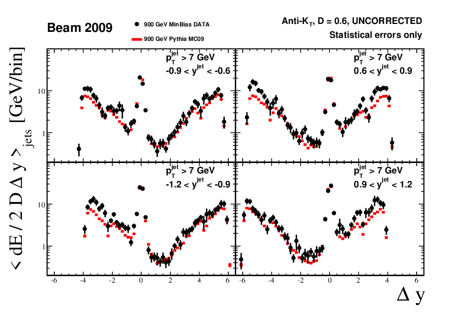

The measured energy flow present the expected peak around the jet axis, and outside the jet cone the energy flow increases as the distance to the jet increases. The measurements show a structure in that can be correlated with the transition across different calorimeter subsystems with different response. The Monte Carlo simulation (pythia MC09) provides a reasonable description of the core of the jet while systematically underestimates the activity away from the jet. The differences are particularly pronounced in the very forward region of the calorimeter and in the crack regions between calorimeters, and can be attributed to deficiencies in the simulation of the detector material and response to low energy particles.
B.2.3 Energy Profiles beyond the cone of the jet
Finally, the energy profile is defined in a similar way as the differential jet shape but normalized to the area in each annulus, and without dividing, jet-by-jet, by the sum of the transverse momenta in :
| (B.3) |
Only central jets with rapidity in the region and are considered and the measurements are carried out using tracks. The use of tracks instead of calorimeter towers allows studying the particle flow around the jet direction without any bias due to the jet search algorithm employed, or the variations of the calorimeter response and the presence of calorimeter cracks as a function of rapidity. The measurements are compared to Monte Carlo simulations in Fig. B.21. As already mentioned, the Monte Carlo models overestimates the amount of transverse momentum close to the core of the jet. The different pythia samples provide a reasonable description of the activity in the region away from the jet axis while phojet underestimates it.


Appendix C Energy Flow
The study of the energy flow away from the jet direction as described in Appendix B was also performed in collisions at TeV at detector level.
Figures C.1 and C.2 show the measured energy flow using tracks and calorimeter clusters respectively, for jets with and . Figure C.3 extend in rapidity the measurement using clusters up to . As expected, the measured energy flow increases due to the presence of a second jet as tends to . The measurements are compared to different MC predictions. PYTHIA-PERUGIA20101 gives a good description of the data. Both PYTHIA-MC09 and PYTHIA-DW tends to underestimate the activity in the region away from the jet axis, dominated by soft hadronic activity, whereas HERWIG++ tend to overestimate it, specially in the forward region.


Bibliography
- [1]
F. Halzen and A.D. Martin, Quarks and Leptons, Wiley (1984).
David Griffiths, Introduction to elementary particles, Wiley (1987). - [2] R. K. Ellis, W. J. Stirling and B. R. Webber, QCD and Collider Physics, Cambridge University Press (1996).
- [3] http://pdg.lbl.gov/
- [4]
V.N. Gribov and L.N. Lipatov, Pair Annihilation and Deep
Inelastic Scattering in Perturbation Theory, Sov. J. Nucl. Phys. 15, 438 (1972).
G. Altarelli and G. Parisi, Asymptotic Freedom in Parton Language, Nucl. Phys. B 126, 298 (1977).
Y.L. Dokshitzer, “Calculation of the Structure Functions for Deep Inelastic Scattering and Annihilation by Perturbation Theory in Quantum Chromodynamics ”, Sov. Phys. JETP 46, 641 (1977). - [5] W.T Giele, E.W.N. Glover and David A. Kosower, Higher Order Corrections to Jet Cross Sections in Hadron Colliders, Nucl. Phys. B 403, 633 (1993).
- [6] Z. Nagy, Next-to-leading order calculation of three jet observables in hadron hadron collision, Phys. Rev. D68 (2003) 094002.
- [7] Stefano Forte, Parton distributions functions at the dawn of the LHC, arXiv:1011.5247v2 [hep-ph] (2010).
- [8] S. J. Brodsky and G. R. Farrar, Scaling laws at large transverse momentum, Phys. Rev. Lett. 31 (1973) 1153.
- [9] H. D. I. Abarbanel, M. L. Goldberger and S. B. Treiman, Asymptotic properties of electroproduction structure functions, Phys. Rev. Lett. 22 (1969) 500.
- [10] J. Pumplin et al., New generation of parton distributions with uncertainties from global QCD analysis, JHEP 07 (2002) 012, arXiv:hep-ph/0201195.
- [11] A. D. Martin, W. J. Stirling, R. S. Thorne, and G. Watt, Parton distributions for the LHC, Eur. Phys. J. C63 (2009) 189–285, arXiv:0901.0002 [hep-ph].
- [12]
H1 and ZEUS Collaborations, HERAPDF 1.5 (preliminary), H1prelim-10-142, ZEUS-prel-10-018.
https://www.desy.de/h1zeus/combined_results/index.php?do=proton_structure - [13]
R. D. Ball et al., A first unbiased global NLO determination of parton distributions and their
uncertainties, Nucl. Phys. B838 (2010) 136–206, arXiv:arXiv:1002.4407 [hep-ph].
S. Forte, E. Laenen, P. Nason, and J. Rojo, Heavy quarks in deep-inelastic scattering, Nucl. Phys. B834 (2010) 116–162, arXiv:arXiv:1001.2312 [hep-ph]. - [14] V.V. Sudakov, Vertex Parts at Very High Energies in Quantum Electrodynamics, Sov. Phys. JETP 3, 65 (1956).
- [15] B. Melle and P. Nason, The Fragmentation Function for Heavy Quarks in QCD, Nucl. Phys. B 361, 626 (1991).
- [16]
B. Andersson, G. Gustafson, G. Ingelman and T. Sjöstrand, Parton Fragmentation
and String Dynamics, Phys. Rept. 97, 31 (1983).
T. Sjöstrand, Jet Fragmentation of Nearby Partons, Nucl. Phys. B 248, 469 (1984). - [17] B.R. Webber, Simulation of QCD Jets Including Soft Gluon Interference, Nucl. Phys. B 238, 492 (1984).
- [18] T. Sjöstrand et al., JHEP 05 026 (2006).
- [19] The CDF Collaboration, T. Aaltonen et al., Phys. Rev. D 82 034001 (2010).
- [20] P. Z. Skands, CERN-PH-TH-2010-113, arXiv:hep-ph/1005.3457 (2010).
- [21] A. Sherstnev and R. S. Thorne, Eur. Phys. J. C 55 553 (2008).
- [22] ATLAS Collaboration, ATLAS MC tunes for MC09, ATL-PHYS-PUB-2010-002 (2010).
- [23] ATLAS Collaboration, Charged particle multiplicities in pp interactions at s = 900 GeV and 7 TeV in a diffractive limited phase-space measured with the ATLAS detector at the LHC and new PYTHIA6 tune, ATLAS-CONF-2010-031 (2010).
- [24] G. Corcella et al., JHEP 0101 010 (2001).
- [25] J. Butterworth, J. Forshaw and M.Seymour, Z. Phys. C 72 637 (1996).
- [26] M. Bahr et al., HERWIG++ Physics and Manual, Eur. Phys. J. C 58 639 (2008).
- [27] M.L. Mangano et al., JHEP 01 0307 (2003).
- [28] F. Caravaglios, M.L. Mangano, M. Moretti and R. Pittau, A New Approach to Multi-jet Calculations in Hadron Collisions”, Nucl. Phys. B 539, 215 (1999).
- [29] S. Alioli, P. Nason, C. Oleari, and E. Re, A general framework for implementing NLO calculations in shower Monte Carlo programs: the POWHEG BOX , arXiv:1002.2581 [hep-ph].
- [30] Gavin P. Salam, Towards Jetography, arXiv:0906.1833v2 [hep-ph] (2010).
- [31] M. Cacciari, G. Salam, and G. Soyez, The anti-kt jet clustering algorithm, JHEP 0804 063 (2008).
- [32] The ATLAS Collaboration, The CERN large hadron collider: accelerator and experiments, JINST 3 (2008) S08001.
- [33] The ATLAS Collaboration, The ATLAS Experiment at the CERN Large Hadron Collider, JINST 3 (2008) S08003.
- [34] The ATLAS Collaboration, Studies of the performance of the ATLAS detector using cosmic-ray muons, Eur. Phys. J. C 71 (2011) 1593.
- [35] W. Lampl et al., Calorimeter Clustering algorithms: Description and Performance, ATLAS-LARG-PUB-2008-002 (2008).
- [36] P. Adragna et al., Testbeam studies of production modules of the ATLAS Tile calorimeter, Nucl. Instrum. Meth. A 606 (2009) 362–394.
- [37]
E. Abat et al., Combined performance studies for electrons at the 2004 ATLAS combined test-beam, JINST 5 (2010) P11006.
M. Aharrouche et al., Measurement of the response of the ATLAS liquid argon barrel calorimeter to electrons at the 2004
combined test- beam, Nucl. Instrum. Meth. A614 (2010) 400–432.
J. Colas et al., Response Uniformity of the ATLAS Liquid Argon Electromagnetic Calorimeter, Nucl. Instrum. Meth. A 582 (2007) 429–455, arXiv:0709.1094 [physics.ins-det].
M. Aharrouche et al., Energy Linearity and Resolution of the ATLAS Electromagnetic Barrel Calorimeter in an Electron Test-beam , Nucl. Instrum. Meth. A 568 (2006) 601–623. - [38]
M. Aharrouche et al., Study of the response of ATLAS electromagnetic liquid argon calorimeters to
muons, Nucl. Instrum. Meth. A606 (2009) 419–431.
ATLAS Collaboration Collaboration, G. Aad et al., Readiness of the ATLAS Tile Calorimeter for LHC collisions, Eur.Phys.J. C70 (2010) 1193–1236, arXiv:1007.5423 [physics.ins-det]. - [39] The ATLAS Collaboration, Luminosity Determination in Collisions at TeV Using the ATLAS Detector at the LHC, Eur.Phys.J.C71:1630 (2011).
- [40] Eur. Phys. J. C 71 2 1512 (2011).
- [41] The ATLAS Collaboration, Measurement of inclusive jet and dijet cross sections in proton-proton collision data at 7 TeV center-of-mass energy using the ATLAS detector, ATLAS-CONF-2011-047 (2011).
- [42] The ATLAS Collaboration, G. Aad et al., Eur. Phys. J. C 70 823 (2010).
- [43] S. Agostinelli et al., Nucl. Instrum. and Meth. A506 250 (2003).
- [44] G. Folger and J.P. Wellisch, arXiv:nucl-th/0306007 (2003).
- [45] H. Bertini, Phys. Rev. 188 1711 (1969).
- [46]
E. Abat et al., Tech. Rep. ATL-CAL-PUB-2010-001, CERN, Geneva, (2010).
P. Adragna et al., CERN-PH-EP-2009-019; ATL-TILECAL-PUB-2009-009 (2009).
E. Abat et al., Nucl. Instrum. and Meth. A607 372 (2009).
E. Abat et al., Nucl. Instrum. and Meth. A615 158 (2010).
E. Abat et al., Nucl. Instrum. and Meth. A621 134 (2010). - [47]
J. Pinfold et al., Nucl. Instrum. Meth. A593 324 (2008).
D. M. Gingrich et al., J. Inst. 2 no. 05 P05005 (2007). - [48] ATLAS Collaboration, Jet energy scale and its systematic uncertainty in proton-proton collisions at sqrt(s)=7 TeV in ATLAS 2010 data, ATLAS-CONF-2011-032 (2011).
- [49] ATLAS Collaboration, In-situ jet energy scale and jet shape corrections for multiple interactions in the first ATLAS data at the LHC, ATLAS-CONF-2011-030 (2011).
- [50] ATLAS Collaboration, Data-Quality Requirements and Event Cleaning for Jets and Missing Transverse Energy Reconstruction with the ATLAS Detector in Proton-Proton Collisions at a Center-of-Mass Energy of 7 TeV, ATLAS-CONF-2010-038, (2010).
- [51]
ATLAS Collaboration, ATLAS calorimeter response to single isolated hadrons and estimation of
the calorimeter jet scale uncertainty, ATLAS-CONF-2010-052 (2010).
ATLAS Collaboration, ATLAS Calorimeter Response to Single Isolated Hadrons and Estimation of the Calorimeter Jet Scale Uncertainty, ATL-CONF-2011-028, (2011). - [52] S. D. Ellis, Z. Kunszt and D. E. Soper, Phys. Rev. Lett. 69 3615 (1992).
- [53]
The CDF Collaboration, D. Acosta et al., Phys. Rev. D 71 112002 (2005).
The CDF Collaboration, F. Abe et al., Phys. Rev. Lett. 70 713 (1993).
The D0 Collaboration, S. Abachi et al., Phys. Lett. B 357 500 (1995). - [54]
The ZEUS Collaboration, S. Chekanov et al., Nucl. Phys. B 700 3 (2004).
The ZEUS Collaboration, J.Breitweg et al., Eur. Phys. J. C 8 3 367 (1999).
The H1 Collaboration, C. Adloff et al., Nucl. Phys. B 545 3 (1999).
The ZEUS Collaboration, J.Breitweg et al., Eur. Phys. J. C 2 1 61 (1998). - [55]
The OPAL Collaboration, R. Akers et al., Z. Phys. C 63 197 (1994).
The OPAL Collaboration, K. Ackerstaff et al., Eur. Phys. J. C 1 479 (1998). - [56] M. D ’Onofrio, S. Grinstein, M. Martínez, F. Vives, Jet Shapes and their sensitivity to the Underlying Event and Pile-up, ATL-PHYS-INT-2009-099 (2009). ATLAS notes become INT after being reviewed within the ATLAS collaboration.
- [57] B. Demirkoz, M. Martínez, F. Vives, First Measurements on Jet Shapes and Energy Flows around Jets in ATLAS using pp Minimun Bias data at , ATL-PHYS-INT-2010-048 (2010).
- [58] The ATLAS Collaboration, Properties and internal structure of jets produced in soft proton-proton collisions at , ATLAS-CONF-2010-018 (2010).
- [59] The ATLAS Collaboration, Phys. Rev. D 83 052003 (2011).
- [60] A. Buckley et al., Rivet user manual. arXiv:1003.0694 [hep-ph]
- [61] J. Pumplin et al., JHEP 0207 012 (2002).
- [62] D. Stump et al., JHEP 0310 046 (2003).
- [63] B. Andersson, G. Gustafson and B. Nilsson-Almqvist, Nucl. Phys. B 281 289 (1987).
- [64] ATLAS Collaboration, Charged particle multiplicities in pp interactions for track MeV at 0.9 and 7 TeV measured with the ATLAS detector at the LHC, ATLAS-CONF-2010-046 (2010).
- [65] A complete set of tables for differential and integrated measurements as a function of and are available at the Durham HepData repository
- [66] The ATLAS Collaboration, G. Aad et al., Phys. Lett. B 688 21 (2010). (http://hepdata.cedar.ac.uk).
- [67] The ATLAS Collaboration, Jet Shapes in ATLAS and Monte Carlo modeling, ATL-PUB-2011-010 (2011).
- [68] The ATLAS Collaboration, New ATLAS event generator tunes to 2010 data, ATL-PHYS-PUB-2011-008 (2011).
- [69] G. Aad et al. (ATLAS Collaboration), arXiv:1103.1816v2 [hep-ex] (2011).
- [70] R. Corke, T. Sjöstrand, JHEP 1103 032 (2011), arXiv:1011.1759 [hep-ph].
- [71] This tune includes a minimum of secondary scatters of 4.1 GeV and a value of the inverse proton radius squared of 1.33 GeV2.
- [72]
S. Gieseke et al., Herwig++ 2.5 Release Note, arXiv:1102.1672 [hep-ph].
(see also http://projects.hepforge.org/herwig/trac/wiki/MB_UE_tunes). - [73] The ATLAS Collaboration, First tuning of HERWIG/JIMMY to ATLAS data, ATL-PHYS-PUB-2010-014 (2010).
- [74] T. Gleisberg, S. Hoeche, F. Krauss, M. Schoenherr, S. Schumann, F. Siegert, J. Winter, JHEP 0902 (2009) 007, [arXiv:hep-ph/0811.4622].
- [75] R. Engel, Phojet, Z.Phys. C60 203 (1995).