Quantum key distribution with delayed privacy amplification and its application to security proof of a two-way deterministic protocol

Bit strings are represented as vectors with elements in GF($2$), where GF($q$) is the Galois field with $q$ elements. We use $\vec{k}$ to denote such a vector and $k[i]$ to denote the $i$th bit. We define the projector function $P(\mbox{$\left|\phi\right\rangle$})\equiv\mbox{$\left|\phi\right\rangle$}\mbox{$\left\langle\phi\right|$}$. We denote the Pauli matrices by

and the corresponding eigenstates by $\{\mbox{$\left|0_{w}\right\rangle$},\mbox{$\left|1_{w}\right\rangle$}\}$ where $w=x,y,z$.

We adopt the universal composability definition of security first proposed by Canetti [41]. This definition quantifies the security of a cryptographic primitive in terms of its deviation from the ideal functionality. The notion of universal composability has been extended to the QKD setting [42, 43].

QKD expands a shorter secret key to a longer one. When one round of QKD that is $\epsilon_{1}$-secure expands on a key generated by a previous round of QKD that is $\epsilon_{2}$-secure, the composition of the two rounds is $(\epsilon_{1}+\epsilon_{2})$-secure [43].

In this paper, we consider PA functions that are additive. A function $f:\text{GF}(q)^{N}\rightarrow\text{GF}(q)^{N_{\text{PA}}}$ is said to be additive if $f(\vec{a}+\vec{b})=f(\vec{a})+f(\vec{b})$ for all $\vec{a},\vec{b}\in\text{GF}(q)^{N}$ and the addition operators are defined in the respective fields. For prime $q$, the function $f$ is additive if and only if it can be expressed in the form of matrix multiplication $f(\vec{a})=A\vec{a}$ where addition and multiplication are defined in $\text{GF}(q)$. The “if” part of this statement is obvious. To prove the “only if” part, note that additivity implies linearity when $q$ is prime since every $\vec{a}\in\text{GF}(q)^{N}$ can be expressed as a pure summation of unweighted basis vectors of some basis (e.g., a weighting of $2$ is broken down into a sum of two terms as in $\vec{a}=2\vec{v}=\vec{v}+\vec{v}$, with $\vec{v}$ being a basis vector) and $f(\vec{a})=\sum_{i=1}^{N}f(a[i]\vec{v}_{i})=\sum_{i}a[i]f(\vec{v}_{i})$, where $\vec{v}_{i}$’s are the basis vectors. Thus, the columns of $A$ are $f(\vec{v}_{i})$’s.

We work in $\text{GF}(2)$ throughout the paper and so $q=2$ and we can always consider PA functions of the form $f(\vec{a})=A\vec{a}$. For $q=p^{r}$ being a power of a prime, we can also restrict additive $f$ to be of the same form in the following sense. We may view $\text{GF}(q)$ as a vector space over its subfield $\text{GF}(p)$, since any element of $\text{GF}(q)$ can be written in the form $\sum_{i=1}^{r}\gamma_{i}\beta_{i}$, where $\gamma_{i}\in\text{GF}(p)$, $\beta_{i}\in\text{GF}(q)$, and $\beta_{i}$ cannot be expressed in the form $\gamma\beta_{j}$ for $j\neq i$ and some $\gamma\in\text{GF}(p)$. This means that an element of $\text{GF}(q)$ can be represented as a length-$r$ vector with elements $\gamma_{i}$. Thus, when we express the PA function in the prime field so that $f:\text{GF}(p)^{rN}\rightarrow\text{GF}(p)^{rN_{\text{PA}}}$, the statement that $f$ is additive if and only if $f(\vec{a})=A\vec{a}$ for all $\vec{a}\in\text{GF}(p)^{rN}$ also holds. Of course, this does not mean that $f$ can be expressed as $A\vec{a}$ for all $\vec{a}\in\text{GF}(p^{r})^{N}$.

Note that the number of additive PA functions grows exponentially as $N$ increases. This makes Eve’s job to attack a key distribution scheme more difficult with larger $N$ as she has to make guesses on the PA function to be used by Alice and Bob in order to customize her attack. Also, additivity is not a very strong constraint and additive functions are commonly used. For example, in Toeplitz matrix based PA [46, 47, 22, 23], the PA function $f(\vec{a})=A\vec{a}$ is additive where $A$ is a Toeplitz matrix.

A property of an additive function $f$ is that any image of $f$ is a translation of the kernel by some offset. This means that the number of elements in every image is the same. We will this property in the proof of Theorem 1.

We note the following special cases:

• •

  (Random message) If the original message $\vec{m}^{\prime}$ is also uniformly chosen (acting as a key), $\vec{m}$ can be uniformly chosen without regard to the condition $\vec{m}^{\prime}=f(\vec{m})$.

• •

  (Imperfect key as message) If the original message $\vec{m}^{\prime}$ is an imperfect key, we can delay the PA of it together with $\vec{a}$. For instance, suppose that $\vec{m}^{\prime}=g(\vec{a^{\prime}})$ is secure after applying the PA function $g$ to the insecure key $\vec{a^{\prime}}$. Then, the encrypting party can send $\vec{a}\oplus\vec{m}$, where $\vec{m}$ is uniformly chosen among all strings that satisfy $g(\vec{a^{\prime}})=f(\vec{m})$.

To apply the delayed PA scheme, given the original message $\vec{m}^{\prime}$, Alice needs to compute its inverse by choosing $\vec{m}$ uniformly among all strings that satisfy $\vec{m}^{\prime}=f(\vec{m})$. Here, we offer a method that Alice can use to compute the PA-inverse $\vec{m}$. Note that this is one possible method, there may be other methods with different efficiencies to perform the same task.

Our method goes as follows. Since $f$ is imposed to be additive, it can be represented by a matrix multiplication in $\text{GF}(2)$, the finite field of two elements:

where $A$ is an $N_{\text{PA}}\times N$ matrix with entries in $\text{GF}(2)$. Multiplication of two elements is AND⁴⁴ 4 AND is an operation on two bits such that $i$ AND $j=1$ only when $i=j=1$., while addition is XOR.

We assume that the rows of $A$ are linearly independent. Thus, we can apply row operations (XOR of two rows) based on Gaussian elimination to express $A$ in upper triangular form:

where the last row has $N_{\text{PA}}-1$ zeros at the beginning and $R$ is an $N_{\text{PA}}\times N_{\text{PA}}$ matrix representing the row operations with $RR=I$. Thus, given $R\vec{m}^{\prime}$, we can find $\vec{m}$ by randomly choosing the last $N-N_{\text{PA}}$ elements of $\vec{m}$ and successively determining the remaining elements of $\vec{m}$ by using the triangular structure.

Suppose Bob and Charlie want to establish a secret key, but they do not have a direct quantum link with each other. Instead, Bob has a quantum link with Alice (a relay) who has already shared a huge supply (denoted as pool $\mathcal{P}$) of perfectly secure⁵⁵ 5 We assume for simplicity that the perfectly secure key is established by face-to-face key exchange. key bits with Charlie. Normally, Alice and Bob would run BB84 to generate from an $N$-bit raw key $\vec{a}$ an $N_{\text{PA}}<N$-bit final key $f(\vec{a})$. With this key, Alice can OTP-encrypt $N_{\text{PA}}$ bits from pool $\mathcal{P}$ and send the cipher text $f(\vec{a})\oplus\vec{m}^{\prime}$ to Bob, where $\vec{m}^{\prime}$ denotes the bits from the pool. Bob then recovers the confidential message $\vec{m}^{\prime}$ that Charlie knows and this completes the task of sharing a key between Bob and Charlie through Alice. If the key $f(\vec{a})$ is $\epsilon$-secure against Eve according to the universally composable definition in Definition 1, the originally perfectly secure key $\vec{m}^{\prime}$ now becomes $\epsilon$-secure.

Suppose that the costs of classical communication, computation, and/or energy of Alice are high. PA can be costly in these aspects. In particular, performing PA requires one party to transmit the full specification of the PA function $f(\cdot)$ to the other party. For example, Toeplitz matrix based PA needs $N+N_{\text{PA}}-1$ bits to specify [46, 47, 22, 23], which can be a big number when the block size is large. Also, performing Toeplitz matrix based PA requires large matrix multiplication, which translates to large computation and energy needs. These can be costly for a satellite relay, for example. In order to reduce these costs, Alice and Bob can delay PA and turn it over to Bob and Charlie. To illustrate the idea of delayed PA, we assume for simplicity that bit and phase error testing and error correction are performed between Alice and Bob as normal. Based on the phase error rate, Bob as in the normal situation decides a particular PA function $f$. But instead of telling Alice about $f$, Bob tells Charlie about it. Now, with delayed PA, Alice can take $N$ bits from pool $\mathcal{P}$ and directly OTP-encrypt them with the raw key $\vec{a}$. This $N$-bit cipher text $\vec{a}\oplus\vec{m}$ is transmitted to Bob, where $\vec{m}$ denotes the $N$ bits from the pool. Bob recovers $\vec{m}$, which Charlie knows. Both Bob and Charlie apply PA $f$ to share a final secret key $f(\vec{m})$, which has length $N_{\text{PA}}$ and is $\epsilon$-secure according to Theorem 1. This generates the same key as in the normal situation without delayed PA. Note that in this example, we sacrifice more key bits between Alice and Charlie to save the communication, computation, and/or energy costs of Alice.

Here, we outline the steps of the BB84 protocol and OTP, which serve as the starting point of the conversion process.

We can view the line from Bob to Alice as a BB84 key distillation step. The steps of BB84 are shown below, where we assume for simplicity the use of quantum memory to avoid the step of discarding bits measured with inconsistent bases.

Protocol 1 (BB84 with quantum memory) on line B-to-A:

1. 1.

   Bob sends $N+N_{\text{test}}$ qubits to Alice taken in $\{\mbox{$\left|0_{z}\right\rangle$},\mbox{$\left|1_{z}\right\rangle$},\mbox{$\left|0_{x}\right\rangle$},\mbox{$\left|1_{x}\right\rangle$}\}$.

2. 2.

   Alice stores all $N+N_{\text{test}}$ received qubits in quantum memory.

3. 3.

   Bob announces the basis of each qubit, and Alice measures her qubits in the corresponding bases.

4. 4.

   Alice and Bob randomly select $N_{\text{test}}$ test bits to find out the bit error rate $e_{b}$ and phase error rate $e_{p}$ for this line B-to-A.⁷⁷ 7 The average quantum bit and phase error rates $e_{b}$ and $e_{p}$ are related to the classical bit error rates in the $x$ basis test bits and the $z$ basis test bits, denoted as $e_{x}$ and $e_{z}$ respectively. Asymptotically, the quantum bit error rate and the phase error rate for the remaining $x$ ($z$) basis bits are $e_{x}$ and $e_{z}$ respectively ($e_{z}$ and $e_{x}$ respectively). Thus, the average quantum bit error rate is $e_{b}=(e_{x}+e_{z})/2$ and the average quantum phase error rate is $e_{b}=(e_{z}+e_{x})/2$. Even though they are the same, we use separate symbols for them to emphasize their meanings in secret key distillation. Alice and Bob choose a privacy amplification function $f(\cdot)$ that is additive and maps $N$ bits to $N_{\text{PA}}=N(1-h(e_{p}))$ bits.

5. 5.

   The final secret key is derived from Alice’s raw key as an $N_{\text{PA}}$-bit string $\vec{k}=f(\vec{a})$. To allow Bob to obtain the same final key, Alice sends Bob $N_{\text{EC}}=Nh(e_{b})$ bits of error correction information encrypted with pre-shared secret bits of the same size so that Bob can correct his raw key $\vec{b}$ to become $\vec{a}$. He then applies the same privacy amplification function $f(\cdot)$ to get the final key $\vec{k}$.

Now, according to Koashi’s security proof of the BB84 protocol [12] (see also other proofs [6, 7, 8, 9]), the final key $\vec{k}$ is secure against Eve with the the net key expansion length as

We can view the line from Alice to Bob as a one-time pad encryption step.

1. 6.

   Alice encrypts an $N_{\text{PA}}$-bit message $f(\vec{m})$ with the secret key $\vec{k}$ with one-time pad and sends the encrypted message $f(\vec{m})\oplus\vec{k}$ to Bob over a classical channel. (As we will see later, $\vec{m}$ will be chosen randomly with uniform probabilities.)

2. 7.

   Bob decrypts his received data with key $\vec{k}$ to get the secret message $f(\vec{m})$.

Here, Eve sees $f(\vec{m})\oplus\vec{k}$ on line A-to-B and the message $f(\vec{m})$ is secure against her because of the security of one-time pad [28].

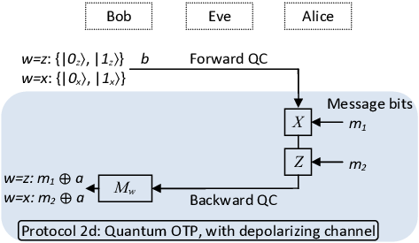
We successively convert the original Protocol 2 to new Protocols 2b, 2c, and 2d, while maintaining the same security in each step to finally arrive at the two-way DQKD protocol. Figure 3 shows the equivalent protocols and they are described in more detail in the following.

1. 6.

   Alice encrypts an $N$-bit random message $\vec{m}$ with her raw key $\vec{a}$ with one-time pad and sends the encrypted message $\vec{m}\oplus\vec{a}$ to Bob over a classical channel line A-to-B.

2. 7.

   Bob recovers the secret message $f(\vec{m})$ as follows. He applies privacy amplification to his received bits to get $f(\vec{m}\oplus\vec{a})$. Due to the additivity of $f(\cdot)$, his received data is $f(\vec{m})\oplus f(\vec{a})=f(\vec{m})\oplus\vec{k}$ which he can decrypt with the same key $\vec{k}$ to recover the message $f(\vec{m})$. Alternatively, he can XOR his received string $\vec{m}\oplus\vec{a}$ with the raw key $\vec{a}$ and apply privacy amplification $f$ to recover the message $f(\vec{m})$.

Here, Eve sees $\vec{m}\oplus\vec{a}$ and this is different from the situation in Protocol 2. Nevertheless, as we have shown in Theorem 1, the security of $f(\vec{m})$ is the same as that in Protocol 2, meaning that Eve cannot get any information about $f(\vec{m})$.

Line A-to-B is now regarded as a quantum channel, even though we use it for the communication of the classical OTP-encrypted message. We encode the OTP-encrypted classical message in Step 6 of Protocol 2b $\vec{m}\oplus\vec{a}$ in a quantum state so that it can be carried by the quantum channel. This is easily done by encoding each bit in the eigenstate of some basis. Here, we assume that the basis used is the same basis $w=x,z$ Bob used to encode his qubit on line B-to-A. Also, we assume for simplicity that Alice knows $w$ for each bit. Thus, the $N$-qubit state Alice sends is $\mbox{$\left|(\vec{m}\oplus\vec{a})_{\vec{w}}\right\rangle$}\equiv\bigotimes_{i}\mbox{$\left|(m[i]\oplus a[i])_{w[i]}\right\rangle$}$ where the index $i$ denotes the $i$th bit for the message, key, and basis. The modified steps are as follows:

1. 6.

   Alice encrypts an $N$-bit random message $\vec{m}$ with the raw key $\vec{a}$ with one-time pad and sends the encrypted message $\left|(\vec{m}\oplus\vec{a})_{\vec{w}}\right\rangle$ to Bob over the quantum channel line A-to-B.

2. 7.

   Bob measures the $N$ qubits received from line A-to-B in basis $\vec{w}$ to recover the OTP-encrypted message $\vec{m}\oplus\vec{a}$. He recovers the secret message $f(\vec{m})$ as in Step 7 of Protocol 2b.

In the previous Protocol 2c, the measurement by Alice disentangles line B-to-A and line A-to-B. Therefore, to come up with an equivalent protocol without a measurement, we need to reproduce this disentanglement feature and at the same time achieve the same overall state in Eq. (6). One way to do this is by replacing the measurement by a depolarizing channel. Starting with the same initial state $\mbox{$\left|\Psi\right\rangle$}_{A\bar{A}}$ for the $i$th bit as in the previous subsection, Alice performs randomly with uniform probabilities the operations, $I$, $X$, $Y$, or $Z$ on each of her $N$ qubits independently. We express this random operation as Alice using a mixed state $4^{-1}\sum_{m_{1},m_{2}=0,1}\mbox{$\left|m_{1}m_{2}\right\rangle$}_{M_{1}M_{2}}\mbox{$\left\langle m_{1}m_{2}\right|$}$ to control the four operations on system $A$:

Here, we assume Alice holds the purification of this mixed state. Tracing the right hand side over $M_{1}$ or $M_{2}$, simple calculations (see Appendix A) lead to

Note that Eqs. (8) and (9) are expressed in terms of bases $z$ and $x$ respectively, regardless of the actual basis $w$ used by Bob to encode system $A$.

We argue that Protocol 2c and Protocol 2d are the same as follows. Eqs. (8) and (9) represent the final overall state of Protocol 2d and we compare them to that of Protocol 2c in Eq. (6). We can see that when $w=z$ ($w=x$), we can identify $m_{1}$ in Eq. (8) (Eq. (9)) with $m$ in Eq. (6). Thus, when $w=z$ ($w=x$), we can regard that Alice’s message bit is in $m_{1}$ ($m_{2}$). Once the basis $w$ is publicly announced by Bob, all of Alice, Bob, and Eve will know whether $m_{1}$ or $m_{2}$ will be used by Alice; in other words, they will know which of Eqs. (8) and (9) describes the situation. Therefore, Protocol 2c and Protocol 2d are the same from Eve’s and Bob’s points of view.

In Protocol 2d, we need a step for Bob to inform Alice about $w$ so that she knows whether $m_{1}$ or $m_{2}$ is her message bit. Note that when Alice performs one of the four operations of the depolarizing channel, she does not know what the message bit value is (unless $m_{1}=m_{2}$). After Bob receives his qubit, he announces to Alice his basis choice $w$ and only then does Alice know the value of her own message bit.

The modified steps of Protocol 2d are as follows:

1. 6.

   Alice chooses two $N$-bit random messages $\vec{m_{1}}$ and $\vec{m_{2}}$. For each qubit received from line B-to-A, she applies $Z$ if $m_{2}=1$ and applies $X$ if $m_{1}=1$.⁸⁸ 8 Note that the order of applications of these two operations does not matter in light of Eq. (7) as swapping the order contributes a factor of $-1$ twice. The qubit is then forwarded back to Bob via line A-to-B.

2. 7.

   Bob measures the $N$ qubits received from line A-to-B in basis $w$ which he has used in Step 1.

3. 8.

   Bob announces to Alice the basis for each qubit. If the basis is $z$ ($x$), Alice’s message bit is $m_{1}$ ($m_{2}$). So in the previous step, Bob’s measured qubit corresponds to Alice’s OTP-encrypted message bit $m_{1}\oplus a$ (for $w=z$) or $m_{2}\oplus a$ (for $w=x$). He recovers the secret message $f(\vec{m})$ as in Step 7 of Protocol 2b, with the appropriate substitution $m_{1}\rightarrow m$ or $m_{2}\rightarrow m$ for each bit. Alice also constructs the secret message $f(\vec{m})$ with the same substitution.

Therefore, when line A-to-B is noiseless, Alice and Bob will share the message bit $m_{1}$ (for $w=z$) or $m_{2}$ (for $w=x$). When line A-to-B is noisy, we can add further error testing and error correction for $\vec{m}$, which we have omitted for simplicity of discussion. Finally, we note that combining Protocol 1 and Protocol 2d essentially gives Protocol DQKD given in Sec. IV.⁹⁹ 9 The key bit error testing of Step 6 of Protocol DQKD is omitted in Protocol 2d for simplicity of discussion, but this step can easily be added without affecting the result. Thus, we have proved the security of Protocol DQKD.

We remark that it makes sense that Alice’s message bit depends on the basis used by Bob. Because when Bob initially sends, for example, a $z$-eigenstate to Alice via line B-to-A, only Alice’s $X$ operation (controlled by $m_{1}$) will bit flip the state, and so $m_{1}$ should become her message bit.

In Protocols 2, 2b, 2c, and 2d, we assume that the final key is derived from applying privacy amplification to Alice’s raw key: $\vec{k}=f(\vec{a})$. Bob is responsible for correcting his raw key to match Alice’s. To ensure security, Alice’s message $\vec{m}$ is shortened to $N_{\text{PA}}=N(1-h(e_{p}))$ bits of secure message $f(\vec{m})$, where $e_{p}$ is obtained from Step 4 of Protocol 1. In the discussion so far, we have not considered errors on line A-to-B. Errors on line B-to-A cause Alice’s raw key to be different from Bob’s raw key such that $\vec{b}=\vec{a}\oplus\vec{e_{1}}$, where $\vec{e_{1}}$ is the error pattern with an error rate of $e_{b}$ (cf. Step 4 of Protocol 1). Errors on line A-to-B cause Bob to receive $\vec{m}\oplus\vec{a}\oplus\vec{e_{2}}$ in Step 6 of Protocol 2b, where $\vec{e_{2}}$ is the error pattern on this line and could be correlated with $\vec{e_{1}}$. Thus, when Bob uses $\vec{b}$ to decrypt his message received on line A-to-B, he faces the error pattern $\vec{e_{1}}\oplus\vec{e_{2}}$, whose error rate we denote as $e_{b}^{\rightleftarrows}$. To help Bob correct for this error pattern, Alice sends to Bob error correction information encrypted with $N(e_{b}^{\rightleftarrows})$ bits of the pre-shared secret key. Therefore, the net key expansion length is

This represents the key generation rate for the integration of Protocol 1 and any of Protocols 2, 2b, 2c, and 2d. As expected, this is the same formula for the two-way DQKD protocol given in Eq. (4) . As a special case, when the error rates on the two lines are both $e_{b}$, the overall error rate $e_{b}^{\rightleftarrows}$ is upper-bounded by $2e_{b}$ since the errors on the two lines can be correlated. Thus, the key generation rate in this case is $1-h(2e_{b})-h(e_{p})$, which is the same as that derived for another two-way DQKD protocol in Ref. [40] (see Sec. III F therein).

Note that as Alice and Bob are correcting the overall error pattern $\vec{e_{1}}\oplus\vec{e_{2}}$, they do not need to separately correct for the error $\vec{e_{1}}$ in their raw keys; i.e., they do not perform Step 5 of Protocol 1. This is reflected in the original two-way DQKD protocol in Sec. IV.

References

- [1] C. H. Bennett and G. Brassard, in Proc. of IEEE Int. Conference on Computers, Systems, and Signal Processing (IEEE Press, New York, 1984) pp. 175–179.
- [2] A. K. Ekert, Phys. Rev. Lett. 67, 661 (1991).
- [3] D. Mayers, J. of ACM 48, 351 (2001), preliminary version in Mayers, D. Advances in Crytology-Proc. Crypto ’96, vol. 1109 of Lecture Notes in Computer Science, Koblitz, N. Ed. (Springer, New York, 1996), pp. 343-357.
- [4] E. Biham, M. Boyer, P. O. Boykin, T. Mor, and V. Roychowdhury, in Proc. of the Thirty-Second Annual ACM Symposium on Theory of Computing (ACM Press, New York, 2000) pp. 715–724.
- [5] H. Inamori, N. Lütkenhaus, and D. Mayers, European Physical Journal D 41, 599 (2007).
- [6] H.-K. Lo and H. F. Chau, Science 283, 2050 (1999).
- [7] P. W. Shor and J. Preskill, Phys. Rev. Lett. 85, 441 (2000).
- [8] B. Kraus, N. Gisin, and R. Renner, Phys. Rev. Lett. 95, 080501 (2005).
- [9] R. Renner, N. Gisin, and B. Kraus, Phys. Rev. A 72, 012332 (2005).
- [10] R. Renner and R. König, in Proc. of the Second Theory of Cryptography Conference (TCC) 2005, Lecture Notes in Computer Science, Vol. 3378 (Springer, Berlin, 2005) pp. 407–425.
- [11] D. Gottesman, H.-K. Lo, N. Lütkenhaus, and J. Preskill, Quant. Info. Compu. 5, 325 (2004).
- [12] M. Koashi, New J. Phys. 11, 045018 (2009).
- [13] T. Tsurumaru and K. Tamaki, Phys. Rev. A 78, 032302 (2008).
- [14] N. J. Beaudry, T. Moroder, and N. Lütkenhaus, Phys. Rev. Lett. 101, 093601 (2008).
- [15] C.-H. F. Fung, K. Tamaki, B. Qi, H.-K. Lo, and X. Ma, Quant. Info. Compu. 9, 0131 (2009).
- [16] L. Lydersen and J. Skaar, Quant. Info. Compu. 10, 60 (2010).
- [17] M. Hayashi, Phys. Rev. A 76, 012329 (2007).
- [18] M. Hayashi, Phys. Rev. A 74, 022307 (2006).
- [19] V. Scarani and R. Renner, Phys. Rev. Lett. 100, 200501 (2008a).
- [20] V. Scarani and R. Renner, Lecture Notes in Computer Science 5106, 83 (2008b).
- [21] R. Y. Cai and V. Scarani, New J. Phys. 11, 045024 (2009).
- [22] C.-H. F. Fung, X. Ma, and H. F. Chau, Phys. Rev. A 81, 012318 (2010).
- [23] X. Ma, C.-H. F. Fung, J.-C. Boileau, and H. F. Chau, Computers & Security 30, 172 (2011).
- [24] C. E. Shannon, Bell System Technical Journal 27, 379 (1948).
- [25] C. H. Bennett, G. Brassard, and J.-M. Robert, SIAM J. Comput. 17, 210 (1988).
- [26] C. H. Bennett, G. Brassard, C. Crépeau, and U. M. Maurer, IEEE Trans. Inform. Theory 41, 1915 (1995).
- [27] G. S. Vernam, American Institute of Electrical Engineers, Transactions of the XLV, 295 (1926).
- [28] C. E. Shannon, Bell System Technical Journal 28, 656 (1949).
- [29] X. Ma and N. Lütkenhaus, “Simplified trusted repeater node for quantum key distribution,” US provisional patent application 61/573,137 (2011).
- [30] K. Boström and T. Felbinger, Phys. Rev. Lett. 89, 187902 (2002).
- [31] A. Wójcik, Phys. Rev. Lett. 90, 157901 (2003).
- [32] Q.-Y. Cai, Phys. Rev. Lett. 91, 109801 (2003).
- [33] Q.-Y. Cai and B.-W. Li, Phys. Rev. A 69, 054301 (2004a).
- [34] Q.-Y. Cai and B.-W. Li, Chinese Phys. Lett. 21, 601 (2004b).
- [35] F.-G. Deng and G. L. Long, Phys. Rev. A 69, 052319 (2004).
- [36] M. Lucamarini and S. Mancini, Phys. Rev. Lett. 94, 140501 (2005).
- [37] M. Lucamarini, A. Ceré, G. Giuseppe, S. Mancini, D. Vitali, and P. Tombesi, Open Syst. Inf. Dyn. 14, 169 (2007).
- [38] K. Boström and T. Felbinger, Physics Letters A 372, 3953 (2008).
- [39] S. Pirandola, S. Mancini, S. Lloyd, and S. L. Braunstein, Nature Physics 4, 726 (2008).
- [40] H. Lu, C.-H. F. Fung, X. Ma, and Q.-Y. Cai, Phys. Rev. A 84, 042344 (2011).
- [41] R. Canetti, in Proc. of 42nd IEEE Symposium on Foundations of Computer Science (FOCS) 2001 (IEEE Press, New York, 2001) pp. 136–145.
- [42] M. Ben-Or and D. Mayers, arXiv:quant-ph/0409062 (2004).
- [43] M. Ben-Or, M. Horodecki, D. W. Leung, D. Mayers, and J. Oppenheim, in Proc. of the Second Theory of Cryptography Conference (TCC) 2005, Lecture Notes in Computer Science, Vol. 3378 (Springer, Berlin, 2005) pp. 386–406.
- [44] R. König, R. Renner, A. Bariska, and U. Maurer, Phys. Rev. Lett. 98, 140502 (2007).
- [45] R. Renner, Security of Quantum Key Distribution, Ph.D. thesis, Swiss Federal Institute of Technology (2005), also available in Int. J. Quant. Inf. 6, 1 (2008).
- [46] Y. Mansour, N. Nisan, and P. Tiwari, Theor. Comput. Sci. 107, 121 (1993).
- [47] H. Krawczyk, in Advances in Cryptology - CRYPTO’94, Lecture Notes in Computer Science, Vol. 893 (Springer-Verlag, 1994) pp. 129–139.
- [48] H.-K. Lo, H. F. Chau, and M. Ardehali, J. of Cryptology 18, 133 (2005a).
- [49] W.-Y. Hwang, Phys. Rev. Lett. 91, 057901 (2003).
- [50] H.-K. Lo, X. Ma, and K. Chen, Phys. Rev. Lett. 94, 230504 (2005b).
- [51] X.-B. Wang, Phys. Rev. Lett. 94, 230503 (2005).