Coarse graining Nuclear Interactions 

The NN interaction provides a basic building block of atomic nuclei. A milestone in the development of the field was achieved when the Nijmegen group generated a fit via a partial wave analysis (PWA) to a set of about 4000 NN scattering data with $\chi^{2}/{\rm dof}\lesssim 1$ [1] after charge dependence (CD) effects were incorporated and discarding about further 1000 of $3\sigma$ inconsistent data. The analysis was carried out using an energy dependent potential for which nuclear structure calculations become hard to formulate. Thus, energy independent high quality potentials were produced with almost identical $\chi^{2}/{\rm dof}$ [2, 3]. Among them, the AV18 potential is directly useful for ab initio Monte Carlo calculations up to $A=10$ [4]. While all these potentials differ in their form, in the last years it has been realized that if CM momenta above $\Lambda=400{\rm MeV}$ are explicitly integrated out, the remaining effective interaction has appealing features. The so-called $V_{\rm lowk}$ potentials [5] exhibit an astonishing degree of universality, produce a rather smooth interaction and weaken the strength of the interaction so that Hartree-Fock calculations may be reliable starting points for nuclear structure calculations. In the present talk we adress a suitable formulation of the problem in configuration space.

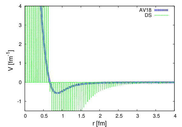
Regarless of these successes it is to date unclear what is the impact of NN uncertainties on finite nuclei due to our ignorance on short distances. Relevant length scales are a) The mean interparticle separation distance $d=1.8{\rm fm}$ as obtained from Nuclear matter saturation density $\rho_{0}=1/d^{3}=0.17{\rm fm}^{-3}$, b) The Fermi momentum $k_{F}=(3/2)^{\frac{1}{3}}/d\sim 250{\rm MeV}$ which gives a wavelength of about $\hbar/k_{F}=0.8{\rm fm}$, c) Minimal relative CM de Broglie wavelengh corresponding to the pion production threshold $\lambda=\hbar/\sqrt{M_{N}m_{\pi}}\sim 0.5{\rm fm}$ and d) The pion Compton wavelength $1/m_{\pi}=1.4{\rm fm}$. The situation is presented pictorially in Fig. 1 suggesting that for the description of the ground state in light nuclei both the short distance core and the role of explicit pions become marginal. This was recognized long ago [6] where the bulk of ${}^{3}{\rm He}$ and ${}^{4}{\rm He}$ could be described with a pionless and soft-core potential which just reproduced the S-wave phase shifts up to $E_{\rm LAB}\leq 100{\rm MeV}$. Actually, we expect this feature to hold for light nuclei.

The basic observation was made long ago by Aviles [7] and recently rediscovered in the context of renormalization of chiral forces [8]. If the two-particle CM wave numbers are limited to a range $\Delta k$ only gross information can be determined in an interval $\Delta r$, (see e.g. Fig. 1) with $\Delta r\Delta k\sim 1$. Thus, for $\Delta k=\Lambda\sim 400{\rm MeV}$ we have $\Delta r_{\rm min}\sim 0.5{\rm fm}$. This uncertainty suggests that for a limited energy range the potential only needs to be known in a limited number of points. With this in mind we consider a neutron-proton (np) potential as a sum of $\delta$ functions

where $\mu=M_{N}/2$ is the reduced np mass of the system, the $\lambda_{i}$ coefficients are strength parameters and $r_{i}$ are the concentration radii. In that case we may determine the s-wave as

where $\delta_{i+1/2}(k)$ is the accumulated phase shift at the mid-point $r_{i+1/2}$ and $\delta(k)\equiv\delta_{N+\frac{1}{2}}(k)$. Matching the discontinuity of log-derivatives at $r=r_{i}$, we simply get

where $U(r)=2\mu V(r)=MV(r)$ is the reduced potential. The regular solution at the origin requires $\delta_{\frac{1}{2}}(k)=0$. If we take the limit $\Delta r\to 0$ we can define $\delta(k,r_{i})=\delta_{i}(k)$, to get

which is the variable phase equation [9] up to finite grid corrections and can be interpreted as the change in the accumulated phase when a truncated potential of the parametric form $U(r)\theta(R-r)$ is steadily switched on as a function of the variable $R$. This equation and its generalization to coupled channels has extensively been used to treat the renormalization problem in NN scattering in Refs. [10, 11, 12]. The low energy expansion of the discrete variable phase equations was used in Ref. [13] to determine threshold parameters in all partial waves. The relation to the well-known Nyquist theorem of sampling a signal with a given bandwidth has been discussed in Ref. [8]. Of course, this DS approximation to the potential can be most immediately used as a numerical method to solve the scattering problem, which would become exact for $\Delta r\to 0$, if we take the weights given by the potential $\lambda_{i}=U(r_{i})\Delta r_{i}$. As an illustration we show in Fig. 2 the phase-shifts obtained for the ${}^{1}S_{0}$-AV18 potential for several values of $\Delta r$. Convergence to the phases to four significant figures is achieved for $\Delta r=0.01{\rm fm}$. The equidistant discretization corresponds to the trapezoidal rule and one could improve by a more sophisticated method, a relevant issue when the interaction is known a priori.

Another, more fruitful and economical, perspective already pursued by Aviles corresponds to consider the weights themselves, $\lambda_{i}$, as fitting parameters to the phase-shifts, since anyhow the potential at short distances is unknown and will be determined from the data.

If we take just one delta-shell in S-wave we may determine both the point $r=r_{c}$ and its corresponding strength, $\lambda_{c}$ from the scattering length $\alpha_{0}$ and the effective range $r_{0}$, defined from

For instance, for the ${}^{1}S_{0}$ case one has $\alpha_{0,^{1}S_{0}}=-23.74{\rm fm}$ and $r_{0,^{1}S_{0}}=2.77{\rm fm}$ which yields $\lambda_{{}^{1}S_{0}}=-0.4626$ and $r_{c,^{1}S_{0}}=1.99{\rm fm}$ whereas for the ${}^{3}S_{1}$ channel one gets $\alpha_{0,^{3}S_{1}}=5.42{\rm fm}$ and $r_{{}^{3}S_{1}}=1.75{\rm fm}$ giving $\lambda_{{}^{3}S_{1}}=-0.911$ and $r_{c,^{3}S_{1}}=1.53{\rm fm}$. The corresponding phase shifts are reproduced to about $E_{\rm LAB}\lesssim 50{\rm MeV}$. One can improve on this by including more delta-shells. A good fit to the PWA is obtained for ($\lambda_{i}$ in ${\rm fm}^{-1}$ and $r_{i}$ in ${\rm fm}$)

This shows that one can consider the grid points as well as the weights as fitting parameters. The result for 5 equidistant points with $\Delta r=0.7\,{\rm fm}$ is shown in Fig. 2 (right panel). Of course, the existence of finite experimental errors helps in decreasing the number of coarse grained grid points.

We have carried out preliminary fits to the NN database [1] with a pion tail with an average $m_{\pi}=138{\rm MeV}$ starting at $2{\rm fm}$ for partial waves with $J\leq 4$ and about 40 parameters with $\chi^{2}/{\rm dof}\lesssim 1-2$. The result for low partial waves is shown in Fig. 3. The full PWA using a CD-OPE potential tail with the pertinent electromagnetic corrections to the PWA database will be presented elsewhere.

It is straightforward to look at the deuteron by analysing the ${}^{3}S_{1}-^{3}D_{1}$ channel for negative energy. The results can be seen in Table 1. The deuteron wave functions as well as the corresponding charge form factor is displayed in Fig. 4. The peaks in the wave functions correspond to the discontinuity in the derivatives at the chosen grid points which, as wee can see, does not become dramatic for the form factor at the considered $q$’s.

Fourier transforming the DS potential in the S-waves gives

which is a finite rank separable potential, a representation which proved very handy in the past for few-body and nuclear matter calculations (see e.g. [14]).

We show in Fig. 5 a comparison of the Fourier transformed DS potentials in the ${}^{1}S_{0}$ and ${}^{3}S_{1}$ channels with with parameters as in Eq. (6) to the corresponding diagonal elements of the $V_{\rm lowk}$ potentials [5], obtained from the AV18 [3] interaction. While the resemblance is indeed rather close, we do not expect a perfect description since the way the scattering problem is treated in the DS case is different as in the $V_{\rm low_{k}}$ case. We have checked that one can represent quite accurately the current diagonal pieces of the $V_{\rm lowk}$ potentials [5] by Eq. (7), but does not necessarily reproduce the off-diagonal matrix elements constructed in the $V_{\rm lowk}$ approach from the truncated the half-off shell Lippmann-Schwinger equation by a specific block-transformation method.

When switching from the NN problem to the many body nuclear problem the features and the form of the interaction are relevant in terms of computational cost and feasibility. We coarse-grain the interaction, but keep the exact kinetic energy, so that for two nucleons at a relative distance $|\vec{x}_{1}-\vec{x}_{2}|\neq r_{c}$ the interaction vanishes, and hence the wave function becomes a Slater determinant of single particle states

We use Harmonic Oscillator single particle wave functions with oscillator parameter $b$, where the spurious CM motion is exactly subtracted, for the shell-configurations ⁴He:$(1s)^{4}$, ¹⁶O:$(1s)^{4}(1p)^{12}$ and ⁴⁰Ca:$(1s)^{4}(1p)^{12}(2s)^{4}(1d)^{20}$. Generally, for double-closed shell nuclei one has

in terms of the relative matrix elements and $g_{nlsj}$ depends on the Talmi-Moshinsky brackets ¹¹ 1 For instance, for ${}^{4}{\rm He}$ one has a m.s.r. $r_{m}=3b/2\sqrt{2}$ and for $R_{1s}(r)=2e^{-\frac{r^{2}}{2b^{2}}}/\sqrt[4]{\pi}b^{3/2}$, $$\langle T\rangle_{{}^{4}{\rm He}}+\langle V_{2}\rangle_{{}^{4}{\rm He}}=3\langle 1s|\frac{p^{2}}{2M}|1s\rangle+6\,\langle 1s|\frac{1}{2}\left(V_{{}^{1}S_{0}}+V_{{}^{3}S_{1}}\right)|1s\rangle=\frac{9}{4b^{2}M}+\frac{6}{b^{3}M}\sqrt{\frac{2}{\pi}}\sum_{n}(\lambda_{n,^{1}S_{0}}+\lambda_{n,^{3}S_{1}})r_{n}^{2}e^{-\frac{r_{n}^{2}}{2b^{2}}}$$ For an Android implementation of these calculations see e.g. http://www.ugr.es/~amaro/android/). Using the single delta function which is just fixed with the S-waves scattering lengths and effective ranges (see below Eq. (5) one obtains at the minimum $B(^{4}{\rm He})=20{\rm MeV}$. In common with other soft potentials [6] the interaction does not require strong correlations in the many-body wave function. This is due to the fact that since the phase-shift is reproduced to about $E_{\rm LAB}=50{\rm MeV}$ the core may be ignored. Clearly, if we insist on reproducing up to $E_{\rm LAB}=350{\rm MeV}$ a strongly repulsive DS contribution emerges and thus a product wave function is not appropriate. One can improve on this by adding more deltas as in Eq. (6) but keeping the fit to $E_{\rm LAB}\leq 100\,{\rm MeV}$, in which case $B(^{4}{\rm He})=24{\rm MeV}$. This is surprisingly close to the Green Function Monte Carlo (GFMC) AV18 [4] and the UCOM method [15] without three-body forces and complies to a cancellation between the core in the and the correlations the wave function.

The results for the binding energy as a function of the corresponding msr radius are presented in Fig. 6. We compare with the UCOM method [15], Brueckner-Hartree-Fock (BHF) [16] and Coupled Cluster (CC) [17]. In the UCOM method [15] a unitary local transformation generates a smooth nonlocal interaction from the AV18-potential while the wave functions are the same. As advertised, our results depend on the fitted energy range, somewhat resembling analogous ambiguities as those of the UCOM.

We have shown how sampling of the NN interaction by a delta shell potential with a resolution determined by the deBroglie wavelength of the most energetic particle provides a coarse graining in configuration space, analogous to the $V_{\rm lowk}$ approach. However, rather than transforming a high quality potential we suggest to determine the NN coarse grained interaction directly from the scattering data. A preliminary fit to the np phase shifts in the Nijmegen data base to all partial waves with $j\leq 4$ requires about 40 fitting parameters yielding $\chi^{2}/\text{d.o.f.}\lesssim 2$ (less than 1 in some waves). Deuteron properties show good agreement with empirical values and other calculations. Harmonic oscillator shell model variational calculations of nuclear binding energies provide results at the 20-30$\%$ accuracy.

The work is supported by Spanish DGI and FEDER funds (grant FIS2008- 01143/FIS) and Junta de Andalucía (grant FQM225). R.N.P. is supported by a Mexican CONACYT grant.

References

- [1] V.G.J. Stoks, R.A.M. Kompl, M.C.M. Rentmeester, and J.J. de Swart. Phys.Rev., C48:792–815, 1993.
- [2] V.G.J. Stoks, R.A.M. Klomp, C.P.F. Terheggen, and J.J. de Swart. Phys.Rev., C49:2950–2962, 1994.
- [3] Robert B. Wiringa, V.G.J. Stoks, and R. Schiavilla. Phys.Rev., C51:38–51, 1995.
- [4] Steven C. Pieper and Robert B. Wiringa. Ann.Rev.Nucl.Part.Sci., 51:53–90, 2001.
- [5] S.K. Bogner, T.T.S. Kuo, and A. Schwenk. Phys.Rept., 386:1–27, 2003.
- [6] I.R. Afnan and Y.C. Tang. Phys.Rev., 175:1337–1345, 1968.
- [7] J.B. Aviles. Phys.Rev., C6:1467–1484, 1972.
- [8] D.R. Entem, E. Ruiz Arriola, M. Pavon Valderrama, and R. Machleidt. Phys.Rev., C77:044006, 2008.
- [9] F. Calogero. Variable Phase Approach to Potential Scattering. Academic Press, New York, 1967.
- [10] M. Pavon Valderrama and E. Ruiz Arriola. Phys. Lett., B580:149–156, 2004.
- [11] M. Pavon Valderrama and E. Ruiz Arriola. Phys. Rev., C70:044006, 2004.
- [12] M. Pavon Valderrama and E.Ruiz Arriola. Annals Phys., 323:1037–1086, 2008.
- [13] M. Pavon Valderrama and E.Ruiz Arriola. Phys.Rev., C72:044007, 2005.
- [14] P. Grygorov, E.N.E. van Dalen, H. Muther, and J. Margueron. Phys.Rev., C82:014315, 2010.
- [15] Thomas Neff and Hans Feldmeier. Nucl.Phys., A713:311–371, 2003.
- [16] H. Muther and A. Polls. Prog.Part.Nucl.Phys., 45:243–334, 2000.
- [17] Jochen H. Heisenberg and Bogdan Mihaila. Phys.Rev., C59:1440–1448, 1999.