Efficient Capacity Computation and Power Optimization for Relay Networks
Abstract
The capacity or approximations to capacity of various single-source single-destination relay network models has been characterized in terms of the cut-set upper bound. In principle, a direct computation of this bound requires evaluating the cut capacity over exponentially many cuts. We show that the minimum cut capacity of a relay network under some special assumptions can be cast as a minimization of a submodular function, and as a result, can be computed efficiently. We use this result to show that the capacity, or an approximation to the capacity within a constant gap for the Gaussian, wireless erasure, and Avestimehr-Diggavi-Tse deterministic relay network models can be computed in polynomial time. We present some empirical results showing that computing constant-gap approximations to the capacity of Gaussian relay networks with around 300 nodes can be done in order of minutes.
For Gaussian networks, cut-set capacities are also functions of the powers assigned to the nodes. We consider a family of power optimization problems and show that they can be solved in polynomial time. In particular, we show that the minimization of the sum of powers assigned to the nodes subject to a minimum rate constraint (measured in terms of cut-set bounds) can be computed in polynomial time. We propose an heuristic algorithm to solve this problem and measure its performance through simulations on random Gaussian networks. We observe that in the optimal allocations most of the power is assigned to a small subset of relays, which suggests that network simplification may be possible without excessive performance degradation.
Index Terms:
capacity, network simplification, power allocation, relay networks, submodular optimization.I Introduction
Relay networks, where one or more source nodes send information to one or more destination nodes with the help of intermediate nodes acting as relays, are often used to model communication in wireless sensor networks. In sensor networks, sensor nodes have limited power sources and often require multi-hop communication with the help of intermediate nodes to reach the data aggregation centers. To guide the design of these networks it is of interest to characterize fundamental communication limits such as the capacity, which represents the maximum reliable communication rate.
Various communication models for relay networks capture in an abstract setting different aspects of practical systems. The wireless erasure network model of [8] captures the effect of packet losses in the wireless setting. The deterministic network model of Avestimehr, Diggavi and Tse (ADT) [4] incorporates broadcast and interference and can be used to gain insights about communication in more complex models that incorporate noise. Among these, of special importance is the Gaussian relay network, which models power limited transmitters and received signals corrupted by additive white Gaussian noise.
While the capacity of some network models (e.g. wireless erasure and ADT) is well characterized, the capacity of the Gaussian relay network, even in its simplest form with one transmitter, one relay, and one receiver, is in general unknown. The best known capacity upper bound is the so-called cut-set bound. A cut of a network can be considered as a subset of nodes which includes the source node and excludes the destination node. For this cut, the capacity is defined as the maximum rate that information can be transferred form the nodes in to the nodes that are not in conditioned on the fact the information on (the nodes that are not in ) is known. The cut-set upper bound is the minimum cut capacity over all the possible cuts.
In the Gaussian setting, there are several capacity lower bounds based on different communication schemes, such as amplify-and-forward, decode-and-forward, compress-and-forward, quantize-and-forward, etc. [5, 7, 18]. Recently, Avestimehr, et al. [2] made significant progress in the capacity characterization of Gaussian relay networks by showing that a quantization and coding communication scheme can achieve a communication rate within a constant gap of the cut-set upper bound, where the gap only depends on the number of nodes in the network (i.e. it is independent of the channel gains and power levels). However, the evaluation of the achievable communication rate, which is necessary to implement the scheme, requires the computation of the cut-set bound for the network. Assuming that for a given cut the cut capacity is easy to compute, finding the cut-set upper bound can be a challenging problem. For a network with relays there are different cuts and a greedy algorithm needs exponential time in the number of relays to compute the cut-set bound.
In this work we show that the achievable rate of the scheme of [2] for the Gaussian relay network can be computed in polynomial time, and as a result, can be computed efficiently. This result is obtained by showing that the cut capacity of a fairly large class of networks under the assumption of independent encoding at the nodes in is a submodular function. For the special case of layered relay networks, [27] showed the equivalent of our submodularity result simultaneously with our conference version of this paper [25]. Submodularity properties of conditional entropy (in terms of which cut-capacities are expressed) have also been used in [2, 3] to bound the cut-capacity of a network in terms of the cut-capacity of the corresponding unfolded graph11 1 Please, refer to [2] for the definition of an unfolded graph..
Existing results on minimization of submodular functions provide algorithms with polynomial running time , where is the time that it takes to compute and is the number of nodes in the network [20]. In addition, there exist possibly faster algorithms without polynomial time performance guarantees based on Wolfe’s minimization norm algorithm [12]. In Section VI, by simulations, we show that the cut-set bound for a Gaussian relay network with around 300 nodes can be computed on a laptop computer in about a minute using a Matlab package for submodular minimization provided in [19].
Our results, extend and generalize previous results for the ADT model. This model can be seen as a high signal-to-noise-ratio (SNR) approximation of the Gaussian model, incorporating the effects of broadcasting and superposition of signals while de-emphasizing the effects of noise. Amaudruz et al. [1] showed that the cut-set bound for a layered22 2 In a layered network, the nodes in one layer are only connected to the nodes in the next adjacent layer. In particular, there is no direct connection from source to destination. ADT model can be computed efficiently. They have extended graph flow algorithms such as Ford-Fulkerson’s in a nontrivial way to find the maximum possible linearly independent (LI) paths in the network. They showed that the capacity of the network is equal to the maximum number of (LI) paths and can be computed in time , where is the maximum number of nodes per layer, is the total number of edges and is the capacity of the network. Moreover, they showed that the capacity can be achieved by using a very simple one-bit processing at the relay nodes. Later Goemans et al. [13] showed that the deterministic model is a special case of a flow model based on linking systems, a combinatorial structure with a tight connection to matroids. As a by-product, they obtained the submodularity of the cut capacity for layered ADT networks. Using this observation they provided various algorithms related to matroid theory to compute the cut capacity of the layered deterministic model based on finding intersection or partition of matroids. These results led to faster algorithms to compute the capacity of large layered ADT networks. In addition, there has been other extensions on improving the running time of the current algorithms for computing the capacity of ADT networks [9, 10, 22, 23].
In addition to showing that the capacity within a constant gap of the Gaussian relay network can be computed in polynomial time, our results allow us to compute in polynomial time the capacity of the wireless erasure network. Furthermore, we provide a simple proof for the computability in polynomial time of the capacity of the layered and non-layered ADT networks.
Building on the submodularity of the cut-capacity for independent encoding at the nodes, we show that, in the Gaussian setting, it is possible to efficiently optimize the power allocated to the source and relay nodes. We consider two power optimization problems: (i) minimize the total power satisfying a minimum source-destination data rate constraint and power constraints at each node; (ii) maximize the source-destination data rate satisfying total and individual power constraints at the nodes. Since the capacity of the Gaussian relay network is approximately given by the cut-set upper bound with independent encoding at the nodes, we use this cut-set bound to characterize data rate in the optimization problems. We show that these optimization problems can be solved in polynomial time and use simulations to get insights about some properties of the optimal power allocations for networks of various sizes. We observe that optimal power allocations assign most of the power to a small subset of nodes and that setting the power to zero in the remaining nodes (i.e. removing these nodes from the network) often results in a small rate loss. Nazaroglu, et al. showed in [26] that for the special case of the -relay Gaussian diamond network a fraction of the total capacity can be approximately achieved by using only of the total relays. This suggests that the diamond network can be significantly simplified by tolerating a small performance loss. Our results provide a numerical counterpart to the fundamental performance bounds derived in [26] and suggest that network simplification may also be possible in more general Gaussian relay networks.
We obtain these results by considering a general framework to compute the cut-set bound. We assign transmit signal random variable to node and we assume the probability distribution over the signals to be independent, i.e . We also assign received signal random variables ’s to each node. The network is defined by the transition probability function . We further assume that the transition probability function is of the form , meaning that the received signals are independent conditioned on the transmitted signals in the network. For such networks we show that 33 3 See Section II for a definition of the notation , , etc. is submodular with respect to . Later we show that for ADT networks, the Gaussian relay network and the wireless erasure network, we can find such that becomes equal to the capacity or the capacity within a constant gap. In other words, the min-cut problem for these networks can be cast as a minimization of a submodular function.
The paper is organized as follows. In Section III we show that for specific type of networks the cut value, , is a submodular function. We then show in Section IV that for many wireless network models such as the ADT deterministic network, Gaussian relay network and wireless erasure network the capacity or an approximation to the capacity can be cast as a minimization of . In Section V we study two power optimization problems and show that they can be solved efficiently. Finally, in Section VI we describe results related to solving optimization problems involving submodular functions and perform power optimization in various randomly generated networks of different sizes. We start by introducing the notation used in the rest of the paper.
II Notation
Let denote the set of nodes in the network and its cardinality. For any subset of nodes we denote by or the set of nodes in that are not in . We assume . A cut is defined as a subset of nodes in . A cut splits the nodes in the network into two groups, the nodes that are in and the ones that belong to . Random variables are shown in capital letters such as and . We use boldface letter for vectors, e.g. is a constant vector and is a random vector. We use to denote with . The function is the mutual information between random variables and conditioned on random variable . With a slight abuse of notation we use to denote either the entropy or differential entropy of the discrete or continuous random variable [6]. By we denote a finite field with elements. Finally, all the functions are in base two.
III Submodularity of cut-set function
Submodularity arises in many combinatorial optimization problems and large body of research has been developed on minimizing or maximizing submodular functions under various constraints.
A submodular function is defined as a function over subsets of with diminishing marginal returns, i.e. if with and any ,
The theorem below establishes the submodularity of the cut capacity function of a general relay network under some special assumptions. This theorem will be used in Section IV to prove that the capacity or an approximation to the capacity of various specific relay network models can be computed by minimizing a submodular function.
Theorem 1.
Consider a network consisting of nodes in . Each node sends a message and receives . If the messages are independent and conditioned on the sent messages the received messages are independent, then the function
is submodular.
Proof.
To show that is submodular we show that is monotonically non-increasing in for .
where (a) is the definition of mutual information and (b) is from the chain rule for the entropy function. Therefore,
where the last equality follows because is independent of conditioned on . So, is non-increasing in and thus is submodular. ∎
In the following example we show that if the signals at the nodes are correlated then is not necessarily a submodular function.
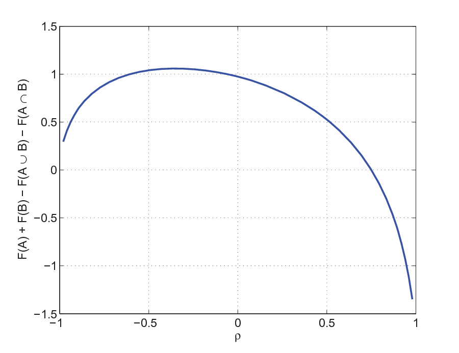
Example. Consider a symmetric Gaussian diamond network with two relays such that the channel gains from source to relays are equal to one and from relays to destination are equal to three. Letting , and be the signals transmitted at the source and relay nodes, then the received signals at relays and destination are given by
where are i.i.d. . For this example, we set the probability distribution of to be jointly Gaussian with zero mean and covariance matrix
Finally, consider the sets and . Figure 1 shows how the function varies for different values of the correlation coefficient (between and ) . We see that can be greater than or less than depending on the value of . It follows that in general is not a submodular or a supermodular function when the there is correlation among the signals at the nodes.
IV Wireless network models
In this section, by applying the result of Theorem 1, we show that the capacity or an approximation to the capacity for the ADT deterministic network, Gaussian relay network, and wireless erasure network can be cast as a minimization of a submodular function.
IV-A Deterministic model (ADT)
We start by briefly describing the network model of [4]44 4 Please, refer [4] for a more complete description of the model and its motivation.. In this model, each link from node to node has an associated non-negative integer gain . Each node transmits a signal and receives a signal , both in where . At any given time, the received signal at node is given by
| (1) |
where is the destination node, the shifting matrix is given by
and the sums and products are in .
For a given cut of the network, where includes the source node and excludes the destination node, we can stack together the input vectors and output vectors , and define a transition matrix that gives the input-output relationship of these vectors according to (1). It is shown in [2] that the capacity of the deterministic network is equal to . We show next in Theorem 2 that is submodular, and hence the capacity can be computed by minimizing a submodular function.
Proposition 1.
Assume an matrix over . Let be the subspace , and let be the set of cosets of in . Pick to be an element in the th coset of for , and set . Notice that if . Now, if we choose uniformly at random from elements of with probability , then the mapping maps to uniformly at random with probability . In addition, the cosets of form a partition of into sets. Also . Thus, .
Theorem 2.
For a deterministic model, given a cut assume is the transition matrix form nodes in to nodes in . Set , then is submodular.
Remark 1.
Proof.
In the network, assume node sends symbols with . We assume ’s drawn i.i.d. with uniform probability distribution over , i.e. for all . From the definition of transition matrix, , if we assume for the cut , symbols are being sent from nodes in and symbols are being received by nodes in then . Then we can write
where is the set of cosets of where . Equality (a) is because is a deterministic function of and (b) is the result of Proposition 1 and the fact the has uniform probability distribution.
Notice that for the independent probability distribution on the sources the received signals are independent conditioned on transmitted signals so, based on Theorem 1, which is equal to is submodular. ∎
IV-B Gaussian relay network
The Gaussian network model captures the effects of broadcasting, superposition and noise of power constrained wireless networks. In this model, at any time index (which we omit) the received signal at node is given by
| (2) |
where is the transmitted signal at node , subject to an average power constraint , is the channel gain from node to node , and is additive white circularly symmetric complex Gaussian noise, independent for different .
It has been show in [21, Theorem 2.1] that using lattice codes for transmission and quantization at the relays, all rates between source and destination satisfying
| (3) |
can be achieved, where is a source-destination cut of the network and are i.i.d. . In addition, the restriction to i.i.d. Gaussian input distributions is within bits/s/Hz of the cut-set upper bound [2]. Therefore the rate achieved using lattice codes in the above result is within bits/s/Hz of the capacity of the network.
The following corollary is an immediate consequence of Theorem 1.
Corollary 1.
The function with the elements of being i.i.d. is submodular.
Due to Corollary 1 the minimization in (3) is the minimization of a submodular function and the resulting optimal value is within of the capacity of the network.55 5 Notice that where is the matrix of channel gains from nodes in to nodes in and is the conjugate transpose of . Therefore, it is easy to compute the capacity of each cut..
IV-C Wireless erasure network
In [8] the authors introduce a special class of wireless networks, called wireless erasure networks. In these networks, a directed graph defines the interconnections between nodes. To model the broadcast effect of wireless networks, the signals on all outgoing arcs of any given node are equal to each other. There is no interference among multiple arcs arriving at a given node in this model, and the signals on the various arcs are erased independently of each other. We assume binary transmitted signals at each node, i.e. , but all the results can be extended to models with larger input alphabets. It has been shown in [8] that the capacity of the network is
| (4) |
where is the probability of erasure when node is sending information to node . We show in the following theorem that is submodular.
Theorem 3.
The function equals where are i.i.d. for . Therefore, is submodular.
Proof.
For i.i.d. , we can write
We used in (a) the independence among and the channel erasures, in (b) the fact that for , , and in (c) the fact that for , and for independent erasures we have . Theorem 1 can be applied to conclude that is submodular. ∎
V Power optimization
In the previous section, for the Gaussian relay network model, we considered fixed power assignments to the different nodes in the network, and have shown that a constant gap approximation to the capacity can be efficiently computed. In many applications it is of interest to allocate the nodes’ transmission powers to optimize a given objective. For example, in a network where the nodes are battery powered, it may be of interest to maximize the network lifetime while satisfying a baseline quality of service. Alternatively, it may be desirable to maximize the network throughput for a given total power budget. This total power budget may arise due to, e.g., a maximum system weight constraint which is dominated by the battery weight, or a total system cost, which may be heavily influenced by the cost of the batteries. Power allocation optimization may also naturally arise in situations where the channel gains, while known to all the nodes, slowly vary over time. In this case, it may be desirable to optimally allocate power for the current channel condition.
As before, we characterize communication rates in terms of cut-set capacities. We consider a model where the cut-set capacities are functions of the cuts and powers assigned to the nodes in the network: , and we focus on the Gaussian model where this function depends explicitly on the power assignment,
| (5) |
where is the matrix of channel gains from nodes in to nodes in , is the conjugate transpose of , and is a diagonal matrix where the diagonal elements are the powers of the nodes in .
We will show in Lemma 1 below that in the Gaussian case is a concave function of . While the results of this section are stated and proved for the Gaussian model, we conjecture that similar results should hold for other models in which is a concave function of .
For Gaussian relay networks, we show that the following optimization problem can be solved in polynomial time,
| subject to | ||||||
| (6) | ||||||
for fixed constants , and . In the rest of the section, we denote the feasible set of the optimization (6) by .
We use the Ellipsoid method [14, 15] to show that the optimization (6) can be solved efficiently. We will use the following definitions and result. The reader is referred to [15] for more details.
Definition 1 (Polynomial computability).
A family of optimization programs is polynomially computable if:
- (i)
for any instance of the program and any point in the domain, the objective and its subgradient can be computed in polynomial time in the size of the instance.
- (ii)
for a given measure of infeasibility , it should be possible to determine if in polynomial time, and when this inequality is not satisfied, it should be possible to find in polynomial time a vector such that
Definition 2 (Polynomial growth).
A family of optimization programs has polynomial growth if the objectives and the infeasibility measures as functions of points in the domain grow polynomially with .
Definition 3 (Polynomial boundedness of feasible sets).
A family of optimization programs has polynomially bounded feasible sets if the feasible set of an instance of the program is contained in an Euclidean ball centered at the origin with radius that grows at most polynomially with the size of the instance.
Proposition 2 ([15, Theorem 5.3.1]).
Let be a family of convex optimization programs equipped with infeasibility measure . Assume that the family is polynomially computable with polynomial growth and with polynomially bounded feasible sets. Then is polynomially solvable.
In order to use Proposition 2 we need to check that the optimization (6) is a convex program. Since the objective function is linear, we only need to check that the feasible set is convex.
Lemma 1.
The feasible set is a convex set.
Proof.
First we show that the function is concave in where for any cut . For any two vectors and we can write
where () is a diagonal matrix where the diagonal elements are the elements of () that belong to (respectively), and (a) follows from the concavity of , for [24].
Next, consider the set . Choose two vectors and in . We will show that is a convex set by showing that for any the vector is also in . Notice that and if and only if and . Therefore
where is due to the fact that is a concave function with respect to . Thus, is a convex set for any .
It is easy to check that the sets , , , and are also convex sets, and, as a result, is a convex set. ∎
Having proved that (6) is a convex program, in order to use Proposition 2 we need to check that the conditions of Definitions 1, 2, and 3 are satisfied. Part (i) of Definition 1 follows from the linearity of the objective in (6). For part (ii) of Definition 1 we specify an infeasibility measure as follows66 6 With a slight abuse of notation we use on vector quantities by taking the maximum over the components of the vector.:
| (7) |
The conditions of part (ii) of Definition 1 are verified in the following theorem.
Theorem 4.
For a given vector and any we can either (a) determine in polynomial time if and if not (b) find in polynomial time a vector , such that for every satisfying , .
Proof.
Part (a) requires checking that each of the arguments of the of (7) is smaller than or equal to in polynomial time. The first six terms are linear functions and can be easily computed. The last term can be compared to by performing a minimization of a submodular function, which as was shown in Section IV-B, can also be computed in polynomial time.
We focus on condition (b). In this case , meaning that at least one of the arguments of the of (7) is larger than . We consider each case separately.
If we set where has a one in the position and zeros everywhere else, which can be easily checked to satisfy the condition of part (b).
Similarly, for the cases , , and we set , , , respectively.
For the last case, let . We have . Since the function is continuous and differentiable with respect to , and the set is convex (which can be shown as in the proof of Lemma 1), then the vector is the normal to a hyperplane that separates from the set . In other words, for all we have . Noting that , we conclude that part (b) holds in this case as well. ∎
Having proved these preliminary results, we are ready to prove the main result of this section.
Theorem 5.
The optimization in (6) can be solved in polynomial time on the size of the problem.
Proof.
The proof uses Proposition 2, which requires verifying the convexity of the problem together with the conditions of polynomial computability, polynomial growth, and polynomial boundedness of the feasible set. Convexity was proved in Lemma 1, while polynomial computability was shown in Theorem 4. Polynomial growth follows from the fact that is the of a polynomial on with degree at most , while the objective and remaining terms that define the infeasibility measure are linear on . Finally, to check that feasible set if polynomially bounded, we note that the feasible set is a subset of the hypercube
where . It follows that the feasible set is contained in the Euclidean ball centered at the origin with radius , which can be easily checked to grow polynomially on the size of the problem. ∎
The general optimization problem (6) can be specialized to a power minimization with a minimum rate constraint, and to a rate maximization with a total power constraint. Both problems can be solved in polynomial time, as stated in the following corollaries to Theorem 5.
Corollary 2.
The following power minimization problem can be solved in polynomial time.
| subject to | ||||||
| (8) | ||||||
Proof.
The corollary follows from Theorem 5 by setting , , . ∎
Corollary 3.
The following rate maximization can be solved in polynomial time.
| subject to | ||||||
| (9) | ||||||
Proof.
The corollary follows from Theorem 5 by setting and . ∎
VI Algorithms and simulations
In this section we study different algorithms and and provide simulation results regarding submodular function minimization and power allocation problems. In the first subsection we look at minimum norm algorithm for submodular function minimization and we show that this algorithm can find the approximation to capacity of layered Gaussian relay networks with more that 300 nodes in a couple of minutes. In the second subsection we propose a heuristic algorithm to find the optimum power allocation for Gaussian relay networks.
VI-A submodular function minimization
One approach to solve the submodular minimization problem due to Lovász is based on extension of the set function to a convex function that agrees with on the vertices of the hypercube , with a guarantee that is equal to for . In this section we assume the normalization .
The Lovász extension of any set function can be defined as follows. For a given order the elements of such that , where is the th element of the vector . Set , , , and
Define and as an dimensional vector such that the coordinates are equal to one and all the other coordinates are equal to zero. Then, it is easy to see that , and . So, is a unique linear convex combination of some vertices of the hypercube and is linear convex combination of values of on those vertices.
A key result is that if is submodular its Lovász extension is a convex function [14, 11]. In addition, finding the minimum of the submodular function over subsets of is equivalent to finding the minimum of the convex function in the hypercube . The optimization can be done in polynomial time using Ellipsoid algorithm [14].
There are other algorithms with faster running time to solve the submodular minimization problem [16, 17, 20]. To the best of our knowledge, the running time of the fastest algorithm is in the order of , where is the time that the algorithms takes to compute for any subset [20]. For ADT networks, Gaussian relay networks, and erasure networks, is the time to compute: the rank of matrices, the determinant of matrices, and equation (4), respectively.
However, for networks of large size, a complexity of may still be computationally cumbersome. As a result, in these cases it is desirable to have faster algorithms. Recently, Fujishing [11, 12] showed that the minimization of any submodular function can be cast as a minimum norm optimization over the base polytope of , , where
and the corresponding minimum norm optimization is
| (10) |
Letting be the solution of this minimization, the set is the solution to . Whether the above optimization problem can be solved in polynomial time is an open problem. However empirical studies [12] have shown that this algorithm has comparable or even faster running times than the other algorithms with polynomial time performance guarantees.

VI-B Power allocation
In Section V we have shown that the Ellipsoid method can be used to solve the optimization in (8) in polynomial time. While in theory this result shows that the optimization in (8) is tractable, in practice the Ellipsoid method has a number of shortcomings that limit its usability. On the one hand the running time of the Ellipsoid method can be large compared to alternative algorithms, and on the other hand, for high dimensional problems it has shown numerical instability. In this section, we propose a heuristic algorithm to solve the optimization in (8) and show that this algorithm converges to the right solution. While the running time can be exponential on the network size, we show through simulations that the algorithm often converges within a time proportional to the network size.
Our proposed algorithm, Algorithm 1 (see pseudo-code below), is based on the cutting plane methods [24] in convex optimization. The optimization in (8) contains exponentially many constraints of the form
| (11) |
In Algorithm 1 we first find the min-cut corresponding to assigning maximum power to all nodes in the network:
Then, we modify the optimization in (8) by replacing the constraint (11) with
The resulting convex program can be easily solved since it contains few constraints.
After optimization, we let be the optimum power allocation for the current set of constraints and set
We iteratively add the constraint
to our set of constraints, and solve the optimization again. We stop if the new constraint is already in the set of constraints.
Since in each iteration the algorithm adds a new constraint to the constraint set and the number of constraints in (11) is finite, the algorithm is guaranteed to find the optimum power in a finite number of iterations, which can be exponential.
We used simulations to test the performance of the algorithm for networks of varying size ranging from 10 to 40. For each , we generated 300 random networks with channels gains drawn i.i.d. using a distribution. We set the desired transmission rate in (8) and set a maximum power constraint in each node to . The results are shown in Figures 3–6, where the the vertical bars represent standard deviation around the mean computed over the 300 random networks.
Figure 3 shows the number of iterations of Algorithm 1 as a function of the number of nodes in the network. We see that the number of iterations grows with the number of nodes.


In Figure 4, we present the simulation time as a function of the network size. We observe a running time that grows slower than . The figure also shows that the power optimization of networks of 40 nodes completes in less than two hours on an Intel Xeon quad core CPU running at 2.33 GHz.
The minimum sum of powers to approximately achieve for networks of different size is presented in Figure 5 with a blue solid line. Interestingly, the plot shows that the minimum power concentrates around the mean. In addition, the figure shows diminishing returns in total power savings resulting from increasing the network size.
For the special case of the diamond relay network with relays, [26] shows that a fraction of the network capacity can be approximately achieved by using only relays. In our setting of a general Gaussian relay network and sum-power minimization, we are interested in investigating whether it is possible to remove a large fraction of the nodes from the network without significantly affecting its performance.
In order to determine which nodes to remove from the network, we solve the sum-power minimization and compare the optimal power allocation of each node to a threshold . All relays with are removed from the network. Let be the set of nodes with . We optimize the power allocation for the network with node set and determine whether the problem is feasible for . If the problem is infeasible, we enlarge by adding more relay nodes in decreasing order of , until the problem becomes feasible.
Figure 5 shows in the red dashed curve the resulting minimum sum of powers obtained by setting . Figure 6 shows the corresponding size of the set . We observe in Figure 6 that the number of nodes with allocated power exceeding (possibly including more relays to make the problem feasible) remains fairly constant as the size of the network increases. This means that most of the power is allocated to a small subset of the nodes.
Removing the remaining nodes from the network and optimizing the power allocation again over the resulting simplified network results in the minimum total power plotted in Figure 5. This figure shows that even though the number of nodes in the simplified network remains approximately constant as increases, the total power required to approximately achieve decreases with . This is due to the fact that larger allows to choose the best relays for the simplified network. There is some performance loss in terms of total power due to network simplification but this loss may be compensated by power savings arising from turning off some of the relays. While we have not modeled the power consumption of the clocks, CPU and other subsystems required to keep a relay active, in practice they may become comparable to the power consumed by radio transmissions. This makes network simplification very useful in practice.
References
- [1] A. Amaudruz and C. Fragouli, “Combinatorial algorithms for wireless information flow,” SODA ’09: Proceedings of the Twentieth Annual ACM-SIAM Symposium on Discrete Algorithms, 2009.
- [2] A. S. Avestimehr, S. N. Diggavi and D. N. C. Tse, “Approximate Capacity of Gaussian Relay Networks,” ISIT ’08: IEEE international Symposium on Information Theory, pp. 474–478, July 2008.
- [3] A. S. Avestimehr, S. N. Diggavi and D. N. C. Tse, “Wireless Network Information Flow: A Deterministic Approach,” IEEE Trans. Info. Theory, vol. 57, no. 4, pp. 1872-1905, April 2011.
- [4] S. Avestimehr, S.N. Diggavi and D. N C. Tse, “A deterministic approach to wireless relay networks,” Forty-Fifth Allerton Conference, Illinois, September 2007.
- [5] Brett E. Schein, Distributed coordination in network information theory, Ph.D. dissertation, Massachusetts Institute of Technology, Cambridge, MA, 2001.
- [6] T. M. Cover and J. A. Thomas, Elements of Information Theory, New York: Wiley, 1991.
- [7] T. M. Cover and A. El Gamal, “Capacity Theorems for the Relay Channel,” IEEE Trans. Info. Theory, vol. 25, no. 5, Sept. 1979, pp. 572–584.
- [8] A. F. Dana, R. Gowaikar, R. Palanki, B. Hassibi, M. Effros, “Capacity of wireless erasure networks,” IEEE Transactions on Information Theory, vol.52, no.3, pp.789–804, March 2006
- [9] J. Ebrahimi, C. Fragouli, “Combinatorial Algorithms for Wireless Information Flow,” under submission in ACM Transactions in Algorithms, 2009. Also available at arXiv:0909.4808v1.
- [10] E. Erez, Y. Xu and E. M. Yeh, “Coding for the Deterministic Network Model,” ITA workshop, San Diego, 2010.
- [11] S. Fujishige, Submodular functions and optimization,(Second Edition), Annals of Discrete Mathematics, Vol. 58, Elsevier, Piscataway, N.J., U.S.A., 2005.
- [12] S. Fujishige, T. Hayashi, and S. Isotani, The Minimum-Norm-Point Algorithm Applied to Submodular Function Minimization and Linear Programming, Kyoto University, Kyoto, Japan, 2006.
- [13] M. X. Goemans, S. Iwata and R. Zenklusen, “An Algorithmic Framework for Wireless Information Flow,” Forty–Seventh Annual Allerton Conference, October 2009.
- [14] M. Groetschel, L. Lovasz, and A. Schrijver, “The ellipsoid method and its consequences in combinatorial optimization,” In Combinatorica, 1:169–197, 1981.
- [15] A. Ben-Tal, and A. Nemirovski, “Lectures on Modern Convex Optimization. Analysis, Algorithms, and Engineering Applications,” SIAM, Philadelphia, PA, 2001.
- [16] S. Iwata, “A faster scaling algorithm for minimizing submodular functions,” SIAM Journal on Computing, 32(4):833–840, 2003.
- [17] S. Iwata and J. B. Orlin, “A simple combinatorial algorithm for submodular function minimization,” In SODA ’09 , pp 1230–1237, 2009.
- [18] G. Kramer, M. Gastpar, and P. Gupta, “Cooperative strategies and capacity theorems for relay networks,” IEEE Transactions on Information Theory, 51(9):3037–3063, September 2005.
- [19] R. A. Krause, Matlab Toolbox for Submodular Function Optimization, http://www.cs.caltech.edu/ krausea/sfo/
- [20] J. Orlin, “A faster strongly polynomial time algorithm for submodular function minimization,” Mathematical Programming, 118(2): 237–251, 2009.
- [21] A. Özgür, and S. Diggavi, “Approximately achieving Gaussian relay network capacity with lattice codes,” to be submitted to IEEE Journal on Selected Areas in Communications, 2010. Available on–line at arXiv:1005.1284v1.
- [22] C. Shi and A. Ramamoorthy, “Improved combinatorial algorithms for wireless information flow,” Forty–Eighth Annual Allerton Conference, pp. 875–880, October 2010.
- [23] S. M. Sadegh Tabatabaei Yazdi and S. A. Savari, “A combinatorial study of linear deterministic relay networks,” IEEE Information Theory Workshop (ITW), pp. 1–5, Jan 6–8, 2010.
- [24] S. Boyd, and L. Vandenberghe, Convex Optimization, Cambridge university press, New York, 2004
- [25] F. Parvaresh and R. Etkin, “On computing capacity of relay networks in polynomial time,” IEEE International Conference on Information Theory (ISIT), pp. 1342–1346, Saint Petersburg, Russia, August 2011.
- [26] C. Nazaroglu, A. Ozgur, J. Ebrahimi, and C. Fragouli, “Wireless Network Simplification: the Gaussian N-Relay Diamond Network with Multiple Antennas,” IEEE International Symposium on Information Theory (ISIT), Saint Petersburg, Russia, pp. 81-85, Aug. 2011.
- [27] A. Raja, and P. Viswanath, “Compress-and-Forward Scheme for a Relay Network: Approximate Optimality and Connection to Algebraic Flows,” IEEE International Conference on Information Theory (ISIT), pp. 1698–1702, Saint Petersburg, Russia, August 2011.